Publisher’s version / Version de l'éditeur:
Vous avez des questions? Nous pouvons vous aider. Pour communiquer directement avec un auteur, consultez la première page de la revue dans laquelle son article a été publié afin de trouver ses coordonnées. Si vous n’arrivez pas à les repérer, communiquez avec nous à [email protected].
Questions? Contact the NRC Publications Archive team at
[email protected]. If you wish to email the authors directly, please see the first page of the publication for their contact information.
https://publications-cnrc.canada.ca/fra/droits
L’accès à ce site Web et l’utilisation de son contenu sont assujettis aux conditions présentées dans le site LISEZ CES CONDITIONS ATTENTIVEMENT AVANT D’UTILISER CE SITE WEB.
Workshop on Autonomous Underwater Vehicles 2004 [Proceedings], 2004
READ THESE TERMS AND CONDITIONS CAREFULLY BEFORE USING THIS WEBSITE.
https://nrc-publications.canada.ca/eng/copyright
NRC Publications Archive Record / Notice des Archives des publications du CNRC :
https://nrc-publications.canada.ca/eng/view/object/?id=a31c3d50-addf-4414-b374-9246f87d303f
https://publications-cnrc.canada.ca/fra/voir/objet/?id=a31c3d50-addf-4414-b374-9246f87d303f
Archives des publications du CNRC
This publication could be one of several versions: author’s original, accepted manuscript or the publisher’s version. / La version de cette publication peut être l’une des suivantes : la version prépublication de l’auteur, la version acceptée du manuscrit ou la version de l’éditeur.
Access and use of this website and the material on it are subject to the Terms and Conditions set forth at
Multi-AUV control and adaptive sampling in Monterey Bay
Fiorelli, E.; Leonard, N. E.; Bhatta, P.; Paley, D.; Bachmayer, R.; Fratantoni,
D.
Proc. IEEE Autonomous Underwater Vehicles 2004: Workshop on Multiple AUV Operations (AUV04), June 2004
Multi-AUV Control and Adaptive Sampling in
Monterey Bay
Edward Fiorelli, Naomi Ehrich Leonard, Pradeep Bhatta, Derek Paley
Mechanical and Aerospace Engineering
Princeton University
Princeton, NJ 08544, USA
{eddie, naomi, pradeep, dpaley}@princeton.edu
Ralf Bachmayer
National Research Council
Institute for Ocean Technology
St. John’s, NL A1B 3T5, Canada
David M. Fratantoni
Woods Hole Oceanographic Institution
Physical Oceanography Department, MS#21
Woods Hole, MA 02543, USA
Abstract— Multi-AUV operations have much to offer a variety of underwater applications. With sensors to measure the envi-ronment and coordination that is appropriate to critical spatial and temporal scales, the group can perform important tasks such as adaptive ocean sampling. We describe a methodology for cooperative control of multiple vehicles based on virtual bodies and artificial potentials (VBAP). This methodology allows for adaptable formation control and can be used for missions such as gradient climbing and feature tracking in an uncertain environment. We discuss our implementation on a fleet of au-tonomous underwater gliders and present results from sea trials in Monterey Bay in August 2003. These at-sea demonstrations were performed as part of the Autonomous Ocean Sampling Network (AOSN) II project.
I. INTRODUCTION
Coordinated groups of autonomous underwater vehicles (AUV’s) can provide significant benefit to a number of appli-cations including ocean sampling, mapping, surveillance and communication. With the increasing feasibility and decreasing expense of the enabling AUV, sensor and communication tech-nologies, interest in these compelling applications is growing and multi-AUV operations are beginning to be realized in the water. Indeed, we report here on results of our tests of multi-AUV cooperative control of a fleet of autonomous underwater gliders in Monterey Bay in August 2003.
In any multi-vehicle task there will likely be spatial scales and temporal scales that are critical to success. For instance, in the case that the AUV group is to function as a communication network, the critical spatial scale may be small since there may
Research partially supported by the Office of Naval Research under grants N00014–02–1–0826 and N00014–02–1–0861, by the National Science Foun-dation under grant CCR–9980058 and by the Air Force Office of Scientific Research under grant F49620-01-1-0382.
be strict limits on how far away individual vehicles can be from one another in order to maintain contact. In certain ocean sensing applications, it may be important to capture ocean dynamics that change quickly and thus short temporal scales may drive the mission. The spatial and temporal scales central to the mission provide a useful way to classify multi-vehicle tasks and the associated vehicle, communication, control and coordination requirements and relevant methodologies.
When each vehicle is equipped with sensors for observing its environment, the group serves as a mobile sensor network. In the case that the mobile sensor network is to be used to sample the physical and/or biological variables in the water, the range of relevant spatial and temporal scales can be dra-matic. Sampling in a relatively large area may be of interest to observe large-scale processes (e.g., upwelling and relaxation) and to understand the influence of external forcing. We refer to the sampling problem for the larger scales as the broad-area coverage problem. As a complement, feature tracking addresses the problem of measuring more local phenomena such as fronts, plumes, eddies, algae blooms, etc.
From one end to the other of the spectrum of scales, multiple AUV’s and cooperative control have much to contribute. How-ever, requirements and strategies will differ. Vehicle endurance will be critical for large-scale activities such as broad-area coverage while vehicle speed may be of particular interest for small-scale efforts such as feature tracking. While vehicle-to-vehicle communication may be impractical for broad-area coverage, it may be feasible for feature tracking. At both ends of the spatial scale spectrum, feedback control and coordination can be central to the effective behavior of the collective. However, the most useful vehicle paths may be different at different scales: e.g., vehicle formations for small scales and coordinated but separated trajectories for large
scales.
There is a large and growing literature on cooperative control in control theory, robotics and biology. For a survey with representation from each of these communities see [6]. There are many fewer examples of full-scale, cooperative multiple-AUV demonstrations in the water. One example by Schultz et al is described in [12].
In this paper we describe cooperative control and adaptive sampling strategies and present results from sea trials with a fleet of autonomous underwater gliders in Monterey Bay during August 2003. These sea trials were performed as part of the Autonomous Ocean Sampling Network (AOSN) II project [2]. A central objective of the project is to bring robotic vehicles together with ocean models to improve our ability to observe and predict ocean processes. New cooperative control and adaptive sampling activities are underway as part of the Adaptive Sampling and Prediction (ASAP) project [1]. Sea trials for this project will take place in Monterey Bay in 2006.
In§IIwe summarize our cooperative control strategy based
on virtual bodies and artificial potentials (VBAP) and discuss its application to feature tracking. VBAP is a general strategy for coordinating the translation, rotation and dilation of an array of vehicles so that it can perform a mission such as climbing a gradient in an environmental field. The challenges and solutions to implementing this strategy on a glider fleet
in Monterey Bay are described in §III. Results from the
Monterey Bay 2003 sea trials are described and analyzed in
§IV. As part of this analysis we evaluate one of the coordinated
multi-vehicle demonstrations for the influence of the sampling patterns on the quality of the data set using a metric based on objective analysis mapping error (equivalently entropic
information). In §V we describe future directions on how we
plan to use this metric to approach optimal design of mobile sensor arrays for broad-area coverage.
II. COOPERATIVECONTROL: VIRTUALBODIES AND
ARTIFICIALPOTENTIALS(VBAP)
In this section we present a brief overview of the virtual body and artificial potential (VBAP) multi-vehicle control methodology. This methodology provides adaptable formation control and is well-suited to multi-vehicle applications, such as feature tracking, in which regular formations are of interest. For example, the methodology can be used to enable mobile sensor arrays to perform adaptive gradient climbing of a sampled environmental field. The general theory for adaptable formation control and adaptive gradient climbing is presented in [9], [10] and specialization to a fleet of underwater gliders in [5].
VBAP relies on artificial potentials and virtual bodies to coordinate a group of vehicles modelled as point masses (with unit mass) in a provably stable manner. The virtual body consists of linked, moving reference points called vir-tual leaders. Artificial potentials are imposed to couple the dynamics of vehicles and the virtual body. These artificial
potentials are designed to create desired vehicle-to-vehicle spacing and vehicle-to-virtual-leader spacing. Potentials can also be designed for desired orientation of vehicle position relative to virtual leader position. With these potentials, a range of vehicle group shapes can be produced [7]. The approach brings the group of vehicles into formation about the virtual body as the virtual body moves. The artificial potentials are realized by means of the vehicle control actuation: the control law for each vehicle is derived from the gradient of the artificial potentials.
The dynamics of the virtual body can also be prescribed as part of the multi-vehicle control design problem. The methodology allows the virtual body, and thus the vehicle group, to perform maneuvers that include translation, rotation and contraction/expansion, all the while ensuring that the formation error remains bounded. In the case that the vehicles are equipped with sensors to measure the environment, the maneuvers can be driven by measurement-based estimates of the environment. This permit the vehicle group to perform as an adaptable sensor array.
VBAP is designed for vehicles moving in 3D space, R3;
for simplicity of presentation, we summarize the case in 2D
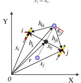
space, R2. Let the position of the ith vehicle in a group of
N vehicles, with respect to an inertial frame, be given by a
vector xi ∈ R2, i = 1, . . . , N as shown in Figure 1. The
position of the kth virtual leader with respect to the inertial
frame isbk∈ R2, fork = 1, . . . , M . The position vector from the origin of the inertial frame to the center of mass of the
virtual body is denoted r ∈ R2. Letxij = xi− xj∈R2 and
hik= xi− bk ∈ R2. The control force on the ith vehicle is
given byui∈ R2. We assume full actuation and the dynamics
can be written fori = 1, . . . , N as
¨ xi= ui.
i
j
x
ix
jr
b
kx
ijh
ik jkh
X
Y
0
jkFig. 1. Notation for framework. Shaded circles are virtual leaders.
Between every pair of vehiclesi and j we define an artificial
potentialVI(xij) and between every vehicle i and every virtual leaderk we define an artificial potential Vh(hik). An additional
of the vectorxi− bk, i.e., the position of vehiclei relative to
the position of virtual leader k. The control law for the ith
vehicle, ui, is defined as minus the gradient of the sum of
these potentials: ui = − N X j6=i ∇xiVI(xij)− M X k=1 (∇xiVh(hik)+ ∇xiVr(θik)).
Typical forms forVI andVh are shown in Figure2. Note that
in this example,VI yields a force that is repelling when a pair
of vehicles is too close, i.e., whenkxijk < d0, attracting when
the vehicles are too far, i.e., when kxijk > d0and zero when
the vehicles are very far apartkxijk ≥ d1> d0, whered0and
d1 are constant design parameters. Examples of Vr(θik) are
presented in [5].
h
ikh
1V
hd
0d
1x
ijV
Ih
0Fig. 2. Representative artificial potentialsVIandVh.
In [7], local asymptotic stability ofx = xeq corresponding
to the vehicles at rest at the global minimum of the sum of the artificial potentials is proved with the Lyapunov function
V (x) = N −1X i=1 N X j=i+1 VI(xij) + N X i=1 M X k=1 (Vh(hik) + Vr(θik)) . (1) This Lyapunov function serves as a formation error function in what is to follow.
To achieve formation maneuvers, dynamics are designed for the virtual body. The configuration of the virtual body
is defined by its position vector r, its orientation R (the 2×2
rotation matrix parameterized by the angle of rotation in the
plane) and its scalar dilation factor k which determines the
magnitude of expansion or contraction. An M -vector φ can
also be defined to fix additional degrees of freedom in the
formation shape using Vr. The design problem is to choose
expressions for the dynamics dr/dt, dR/dt, dk/dt, dφ/dt.
As a means to design the virtual body dynamics to ensure stability of the formation during a mission, the path of the virtual body in configuration space is parameterized by a scalar variable s, i.e., r(s), R(s), k(s), φ(s) for s ∈ [ss, sf]. Then, the virtual body dynamics can be written as
dr dt = dr ds˙s, dR dt = dR ds ˙s, dk dt = dk ds˙s, dφ dt = dφ ds˙s (2)
where ˙s = ds/dt. The formation error defined by (1) becomes
V (x, s) because the configuration of the virtual body, and
therefore the artificial potentials, are a function ofs.
The speed along the path, ˙s, is chosen as a function of the
formation error to guarantee stability and convergence of the
formation. The idea is that the virtual body should slow down if the formation error grows too large and should maintain a desired nominal speed if the formation error is small. Given a
user-specified, scalar upper bound on the formation error VU
and a desired nominal group speed v0, boundedness of the
formation error and convergence to the desired formation is proven with the choice
˙s = h(V (x, s)) +− ∂V ∂x T ˙x δ + |∂V∂s| δ + VU δ + V (x, s) (3)
with initial condition s(t0) = ss, δ 1 a small parameter
and h(V ) = ( 1 2v0 1 + cosπV2UV if |V | ≤ VU 2 0 if |V | > VU 2 .
˙s is set to zero when s ≥ sf.
The remaining freedom in the direction of the virtual body
dynamics, i.e.,dr/ds, dR/ds, dk/ds, dφ/ds, can be assigned
to satisfy the mission requirements of the group. For example, the choice dr ds = 1 0 , dR ds = 0, dk ds = 1
produces a formation that expands linearly in time with its center of mass moving in a straight line in the horizontal direction and its orientation fixed. Stability and convergence of
the formation are guaranteed by the choice of ˙s, independent
of the choice of group mission.
As another possibility, the specification of virtual body direction can be made as a feedback function of measurements taken by sensors on the vehicles. For instance, suppose that
each vehicle can measure a scalar environmental fieldT such
as temperature or salinity or biomass concentration. These measurements can be used to estimate the gradient of the field
∇Test at the center of mass of the group. If the mission is to
move the vehicle group to a maximum in the field T , e.g.,
hot spots or high concentration areas, an appropriate choice of direction is
dr
ds = ∇Test.
This drives the virtual body, and thus the vehicle group,
to a local maximum in T . Convergence results for gradient
climbing using least-squares estimation of gradients (with the option of Kalman filtering to use past measurements) are presented in [9]. The optimal formation (shape and size) that minimizes the least-square gradient estimation error is also investigated. Adaptive gradient climbing is possible; for example, the dilation of the formation (resolution of the sensor array) can be changed in response to measurements for optimal estimation of the field.
The approach to gradient climbing can be extended to drive formations to and along fronts and boundaries of features. For example, measurements of a scalar field can be used to compute second and higher-order derivatives in the field,
necessary for estimating front locations (e.g., locations of maximum gradient).
We note that vehicle groups controlled in regular formations are particularly useful for climbing environmental gradients and other feature tracking missions. Vehicle formations yield spatially distributed measurements which can be used to estimate gradients on spatial and time scales beyond the capabilities of a single vehicle. This is especially relevant for slow moving vehicles like the underwater glider discussed in §III-A.
III. COOPERATIVECONTROL OFAUTONOMOUS
UNDERWATERGLIDERFLEETS
The theory summarized in§IIdoes not directly address
var-ious operational constraints and realities associated with work-ing with real vehicles in the water. In this section we address a number of these issues in a summary of our implementation of the VBAP methodology for a fleet of underwater gliders in Monterey Bay. For example, the control laws are modified to accommodate constant speed constraints consistent with glider motion and to cope with external currents. The implementation also treats underwater gliders which can only track waypoints and can only communicate every couple of hours while at the surface. The details of the implementation are described in [5]. In August 2003, we ran sea trials with a fleet of Slocum autonomous gliders as part of the Autonomous Ocean Sam-pling Network (AOSN) II project. Gliders were controlled in formations using the VBAP methodology with implementation
as described here. Sea-trial results are described in §IV.
A. The Autonomous Underwater Glider
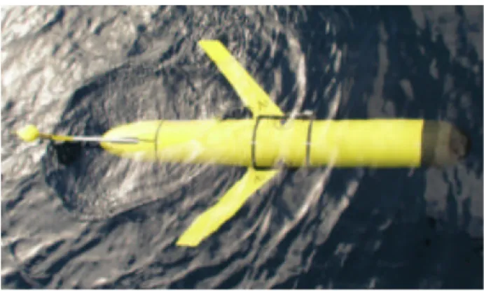
Autonomous Underwater Gliders are a class of energy ef-ficient AUV’s designed for continuous, long-term deployment [11]. Gliders can be significantly less expensive as compared to conventional AUV’s, so they are particularly well-suited to be deployed in large numbers. Furthermore, gliders have high endurance, and as a result are playing an increasingly critical role in autonomous, large-scale ocean surveys [2]. Over the last few years three types of ocean-going underwater gliders have been developed for oceanographic applications: the Slocum [15], the Spray [14], and the Seaglider [4]. A Slocum glider operated by one of the authors (D. Fratantoni) and manufactured by Webb Research Corporation is shown in Figure 3.
The energy efficiency of the gliders is due in part to the use of a buoyancy engine. Gliders change their net buoyancy (e.g., using a piston-type ballast tank) to change their vertical direc-tion of modirec-tion. Actively controlled redistribudirec-tion of internal mass is used for fine tuning attitude. The Slocum uses a rudder for heading control. Fixed wings provide lift which induces motion in the horizontal direction. The nominal motion of the glider in the longitudinal plane is along a sawtooth trajectory where one down-up cycle is called a yo. Having no active thrust elements, gliders are very sensitive to external currents.
Fig. 3. Slocum glider.
The Slocum glider is equipped with an Iridium-based, global communication system and a line-of-sight, high-bandwidth Freewave system for data communication. Both systems are RF-based and subsequently can only be used at the surface.
The Slocum glider operates autonomously, tracking way-points in the horizontal plane. While underwater, the glider uses dead reckoning for navigation, computing its position using its pressure sensor, attitude measurement and integration of its horizontal-plane velocity estimate.
Gliders are inherently sensitive to ocean currents and the Slocum includes the effects of external currents in its dead reckoning algorithms and heading controller. However, during a dive cycle the glider does not have a local current measure-ment. Instead the glider uses a constant estimate computed at the last surfacing by comparing dead-reckoned position with recently acquired GPS fixes. Any error between the two is attributed to an external current. The current information is also made available as science data.
Gliders can be equipped with a variety of sensors for gathering data useful for ocean scientists. The Slocum gliders used in Monterey Bay in 2003 housed sensors for temperature, salinity, depth, chlorophyll fluorescence, optical backscatter and photo-synthetic active radiation (PAR). Sensor measure-ments can be used to drive multi-vehicle feedback control algorithms with the goal of collecting data that is most useful to understanding the environment. This contributes to what is
known as adaptive sampling, discussed in§III-D.
B. Implementation of VBAP for a Network of Gliders As part of the AOSN-II experiment during August 2003, twelve Slocum gliders, operated by Fratantoni, were deployed in Monterey Bay, CA. The Slocum gliders were monitored from the central shore station located at the Monterey Bay Aquarium Research Institute (MBARI) at Moss Landing, CA. Every time a glider surfaced, it communicated via Iridium with the Glider Data System (GDS) at Fratantoni’s lab at the Woods Hole Oceanographic Institution (WHOI) in Massachusetts. The GDS is a custom software suite which provides real-time
monitoring and mission cuing services for multiple-Slocum glider operations. New missions were uploaded to the GDS from MBARI through the internet. Likewise, glider data was downloaded from the GDS to MBARI through the internet. During 2003, each of the gliders surfaced (independently) every two hours. No underwater communication between gliders was available.
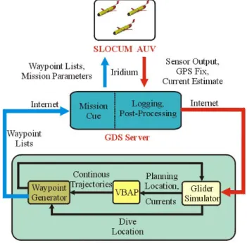
To coordinate fleets of underwater gliders we applied the
general control theory of §II to the seafaring glider AUV’s.
Figure 4 presents a schematic view of the coupled
VBAP-Glider system implemented during AOSN-II.
Fig. 4. AOSN-II VBAP Operational Scenario.
In the implementation, our interface to the Slocum gliders is through the GDS and subsequently the final VBAP output consists of waypoint lists. When a glider surfaces it acquires a GPS fix and then establishes an Iridium connection with the GDS Server at WHOI. The recently acquired GPS fix, sensor profile data, and estimated external currents are uploaded to the GDS server where they go through quality control and are subsequently logged. At any time, the option exists to halt the current mission plan and upload a new one. A mission plan consists of a set of waypoints specified in the horizontal plane, yo depth bounds, and duration after which the glider will begin to surface next. During the coordinated control demonstrations in 2003, we ran VBAP on an on-shore computer to determine a new mission plan once every two hours for all the gliders included in the demonstration. To limit the time spent on the surface by the gliders, mission plans for each glider were to be available immediately at surfacing. Thus, the latest information could not be used for design of the immediate mission plan.
To initialize VBAP, each glider’s location is needed. So that mission plans are immediately available at surfacing, an
estimate is needed of the dive location of each glider at the start of its next mission, denoted dive location. Also needed for each glider is its location when the lead glider dives, denoted planning location. Both sets of locations are necessary because of the possibility of surfacing asynchronicities among gliders in the formation. The lead glider in the group is the glider expected to surface first at the start of the demonstration (cho-sen so that time between surfacings of the lead and the other gliders is small). VBAP generates smooth trajectories and then, from these, sets of waypoints for all gliders simultaneously. The planning locations are used in initializing VBAP. The dive locations are used to ensure the waypoint lists to be generated are consistent with the locations of the other gliders when they actually start the mission.
Both planning and diving locations are generated by a Glider Simulator which is a dynamic simulation using a “black-box” model of the Slocum glider. As its inputs, it uti-lizes the current mission plan, consisting of waypoints, mission duration, and yo depth bounds, last known position before diving, and the currents reported during the last mission. The simulator is fairly detailed and an in-depth discussion of its workings can be found in [5].
VBAP is then initialized with the estimated planning lo-cation for each glider and the average of the last reported estimated currents. VBAP generates a continuous trajectory for each glider which is then discretized into waypoints in the Waypoint Generator. The discretization is performed using constrained minimization of an appropriate cost function [5]. In the process of generating waypoints, we ensure that the new mission waypoints are compatible with the dive locations to avoid undesired backtracking. In particular, if the output of the waypoint generator is expected to yield backtracking, we have the option of removing the offending waypoints. During
the sea-trials described in§IVthis was never required.
C. Operational constraints and Implementation issues To coordinate glider fleets during AOSN-II numerous issues relating to glider control and actuation, planning and informa-tion latencies, and surfacing asynchronicities were addressed. Constant glider speeds (an AOSN-II constraint) and external currents were two critical glider control and actuation issues. In AOSN II, the Slocum gliders were programmed to servo to a constant pitch angle (down for diving and up for rising). This kind of operation yields speeds relative to external currents that are fairly uniform on time scales which span multiple yos. In this respect, the Slocum glider is suitably modeled as having constant speed. The constant speed constraint was added to the VBAP methodology, with the understanding that this constraint restricts what formations are feasible using VBAP. Numerical simulations have shown that formations that are not kinematically consistent with the speed constraint will lead to VBAP not converging properly. For example, a “rolling” formation defined by a virtual body that is simultaneously translating and rotating is not kinematically consistent with
the constant speed constraint. This is because each vehicle must slow down at some point to be “overtaken” by its neighbor. Convergence problems may also arise for certain initial conditions. For a further discussion of implementation and consequences of the constraint, see [5].
When external currents that vary across the formation are present, the very existence of a formation, i.e. a configuration of vehicles in which all relative velocities between vehicles remains zero, is uncertain. This is an artifact of the assumption that the glider speed is constant relative to the current. We circumvent this problem by using a group average current estimate in the VBAP planner [5]. A related challenge can arise from the practice of using the previous glider current estimate integrated over the entire previous dive cycle for the next dive cycle. Because of this, the glider will find it difficult to navigate through currents which vary greatly over the course of the dive cycle.
As mentioned in §III-B we do not impose synchronous
surfacings of the glider fleet. Variabilities across the glider
fleet such as w-component (vertical) currents and the local
bathymetry, decrease the likelihood of synchronous surfacings occurring naturally. Also, substantial winds and surface traffic (like fishing boats, etc.) render waiting on the surface to im-pose synchronicity impractical and dangerous. As discussed, we generate a plan using VBAP for the entire fleet simulta-neously. For the other gliders, it is tempting to consider not using the plans generated then, but instead to generate new plans based on the latest data from the lead or other glider if available. However, during the replanning process we would have to constrain the trajectories of gliders that have already received their plans and have gone underway. VBAP is not capable of handling such a constraint. Underwater acoustic communication, if implemented, may alleviate this constraint by permitting a replan for vehicles that are already underwater. In this case, there would likely be constraints on the separation distance between gliders to enable effective communication.
Latency was also a significant issue for coordinating glider fleets. During AOSN-II, data sent to the GDS after a glider surfaced was not available in a timely enough manner to be used in the generation of the next mission plan. Therefore GPS fixes and local current estimates were latent by one dive cycle. There are two related issues which arise. First, the external current estimates lag the cycle for which we are planning by two dive cycles. That is, we are using the average current from the previous cycle as a proxy for the current during the cycle after next. Secondly, the currents used to estimate each glider’s diving position lags by one cycle. In regions of moderate to high current variability over the course of the glider’s dive cycle, coordination is hampered due to errors in the glider’s own dead reckoning and navigation.
D. Adaptive Sampling
A central objective in ocean sampling experiments with limited resources is to collect the data that best reveals the
ocean processes and dynamics of interest. There are a number of metrics that can be used to help define what is meant by the best data set, and the appropriate choice of metric will typically depend on the spatial and temporal scales of interest. For example, for a broad area, the goal might be to collect data that minimizes estimation error of the process of interest. For smaller scales, the goal may be to collect data in and around features of interest, e.g., to sample at locations of greatest dynamic variability. A fundamental problem is to choose the paths of available mobile sensor platforms, notably sensor-equipped AUV’s, in an optimal way. These paths, however, do not need to be predetermined, but instead can be adapted in response to sensor measurements. This is called adaptive sampling.
When multiple AUV’s are available, cooperative feedback control is important for enabling adaptive sampling. For exam-ple, in covering a broad region, the AUV’s should be controlled to appropriately explore the region and avoid approaching one another (in which case they would become redundant sensors). For adaptive feature tracking, the formation control
and gradient climbing and front tracking described in§IIcan
be used. Feedback plays several critical roles. First, feedback can be used to redesign paths in response to new sensor mea-surements. Of equal importance, feedback is needed to manage the uncertainty inherent in the dynamics of the vehicles in the water. Using the measurements of vehicle positions and local currents, feedback (e.g., as implemented above) can be used to ensure the AUV’s do what they are supposed to do despite a variety of disturbances.
Adaptive sampling strategies using formations are explored and implemented (using VBAP) in [5]. A library of basic formation maneuvers, such as gradient climbing, zig-zagging in formation across a front, group expansions and rotations, are used as building blocks in scenarios for feature tracking and sampling of “dynamic hot-spots”.
Alternative strategies for cooperative control and adaptive sampling with multiple AUV’s, e.g., for broad-area coverage, are under development.
IV. SEATRIALS: AOSN-II, MONTEREYBAYSUMMER
2003
During the AOSN-II experiment in Monterey Bay in sum-mer 2003 we had the opportunity to demonstrate our co-ordinated control methodology on Slocum glider fleets. In this section we describe three demonstrations and present an evaluation of the coordination performance. During all three demonstrations, each glider surfaced every two hours for a GPS fix and received an updated mission plan. The gliders dove to a depth of 100 meters.
The first two sea-trials performed on August 6, 2003 and August 16, 2003 demonstrate our ability to coordinate a group of three Slocum underwater gliders into triangle formations. In both cases, we used our VBAP methodology with a single virtual leader serving as the virtual body. We explored various
orientation schemes and inter-vehicle spacing sequences as the formation made its way through the bay. During the last demonstration, performed on August 23, 2003, a single Slocum glider was controlled to track the path of a Lagrangian drifter in real-time.
The glider dead reckoning and current estimate histories are post-processed to estimate each glider’s trajectory during the
course of each demonstration. Denote theithglider’s position
at time t in the horizontal plane as gi(t). (Note: gi(t) is
distinguished from xi(t) which refers to the position of the
ith glider at time t as planned by VBAP). The instantaneous
formation center of mass is defined as g(t) =¯
N
P
i=1
1
Ngi(t)
where N is the number of vehicles in the formation. The
inter-vehicle distance between gliders is given by dij(t) =
kgi(t)− gj(t)k where i, j = 1, . . . , N, i 6= j.
With a single virtual leader, the virtual body is a point and therefore has no orientation. In some of the Monterey Bay sea trials, we let the orientation of the formation remain unconstrained. In principle, this means that the formation can take any orientation around the virtual leader as it moves with the virtual leader. In the case of significant currents and limited control authority, this approach allows us to dedicate all the control authority to maintaining the desired shape and size of the formation. Sometimes, however, it is of interest to devote some control authority to control over the orientation. For instance, to maximize trackline separation for improved sampling, we ran some sea trials with one edge of the formation triangle perpendicular to the formation path. In order to effect this, we defined the desired orientation of the formation by constraining the direction of the relative position vectors(xi− r) (the vector from virtual leader to ithvehicle).
Potential functionsVras described in§IIwere used to impose
this constraint.
Let r(t) be the VBAP planned (continuous) trajectory for the virtual leader. Since the virtual body consists only of the one virtual leader, this trajectory is the trajectory of the desired center of mass (centroid) of the formation. A new mission is planned every two hours and defines a two-hour segment of the demonstration; the start of each mission is defined by the time at which the lead glider dives after having surfaced.
Thus, for a demonstration lasting2K hours, VBAP generates
K missions. The formation centroid error at time t is defined as = k¯g(t) − r(t)k, i.e., it is the magnitude of the error between the formation centroid and the virtual leader position
generated by VBAP at timet. We note that this error defines a
rather conservative performance metric because it requires, for good performance, that the formation track the virtual body both in space and in time.
A. Aug 6, 2003: Glider Formation at Upwelling Event On August 6, 2003 three Slocum gliders were coordinated into a triangle formation and directed towards the northwest part of Monterey Bay in response to the onset of an upwelling
event (see Figure 5). The WHOI gliders WE07, WE12, and
WE13, were initially on hold missions at the mouth of the bay and the mission plan was to transit the gliders to the northwest in an equilateral triangle formation with an inter-vehicle spacing of 3 km. The entire demonstration spanned sixteen hours, i.e., eight two-hour missions. During the first four missions the triangle formation was free to rotate about the virtual leader. During the last four missions, the orientation of the group about the virtual leader was controlled so that an edge of the triangle formation would be perpendicular to the group’s path.
Fig. 5. Satellite sea surface temperature (degrees C) in Monterey Bay for Aug 6, 2003 19:02 UTC. Cold water region near the northwest entrance of the bay indicates onset of upwelling event. The three solid circles indicate the starting locations of the Slocum gliders at approximately 18:00 UTC. The solid diamond is the desired destination of the glider group. AVHRR HRPT data provided courtesy of NOAA NWS Monterey Office and NOAA NESDIS CoastWatch program.
Figure 6 presents the glider trajectories and instantaneous
glider formations. Starting from their initial distribution, the gliders expanded to the desired configuration while the forma-tion centroid tracked the desired reference trajectory, i.e. the virtual leader. As shown, the group did maintain formation while transiting. At 02:36:58 orientation control was activated and by 06:55:36 the group had noticeably reoriented itself. As a result of generating waypoint plans that respect a glider with constant speed, some degree of backtracking is seen to occur during the initial creation of the desired formation and during the missions when orientation control was active.
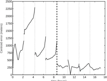
The formation centroid error is plotted over all eight
missions in Figure7 as a function of timet. The mean value
of averaged over all eight missions is 623 meters with a standard deviation of 500 meters. The average error over the last four missions is 255 meters with a standard deviation of 67 meters. The discontinuities at each mission replan is a result of re-initializing the virtual leader at the expected centroid of the group. The error across the discontinuity gives insight into how well we predicted the initial location of the group centroid at the start of each mission. During mission 2 we performed
−122.4 −122.35 −122.3 −122.25 −122.2 36.82 36.84 36.86 36.88 36.9 36.92 36.94 36.96 36.98 Longitude Latitude 18:00:04 20:10:27 22:18:44 00:26:22 02:36:58 04:45:31 06:55:36 09:03:14 11:09:56 WE07 WE12 WE13
Fig. 6. Glider trajectories and snapshots of glider formations. Solid lines are glider trajectories. Black dashed lines illustrate instantaneous formations at 2-hour intervals. Red dotted line is formation centroid. Black dash-dot line is virtual leader’s trajectory (desired trajectory of formation centroid). Time is UTC from August 6, 2003.
worst at predicting initial centroid location and maintaining the distance between the actual and desired centroid location. This error corresponds to the largest error between the current estimates fedforward into the glider simulator and VBAP (see
Figure 4), and the estimated current measured by the gliders
at the end of that mission. We performed best with respect to this metric during the last four missions. It is possible that the difference in performance is related to our observations that during the latter part of the demonstration each glider travelled fastest relative to ground due to more favorable currents in the glider’s direction of travel. Further analysis of these results is in progress. 0 2 4 6 8 10 12 14 16 18 0 250 500 750 1000 1250 1500 1750 2000 2250 2500 time (hours)
Centroid error (meters)
Fig. 7. Formation centroid error vs. time. Black dotted vertical lines indicate
the beginning of each mission. August 6, 2003 demonstration.
Figure8portrays the magnitude of the error in inter-vehicle
distancedij(t) versus time for the three glider pairings
WE07-WE12, WE07-WE13, and WE12-WE13. The mean error of all three pairings is 423 meters, roughly 14% of the desired spacing of 3km, with a standard deviation of 159 meters. The mean inter-vehicle spacing error was largest during missions 2 and 5. 0 2 4 6 8 10 12 14 16 18 0 200 400 600 800 1000 1200 1400 1600 time (hours)
Inter−vehicle distance error (meters)
WE07−WE12 WE07−WE13 WE12−WE13 Mean
Fig. 8. Magnitude of inter-glider distance error vs. time. Black dotted vertical lines indicate the beginning of each mission. August 6, 2003 demonstration.
Formation orientation error versus time is portrayed in
Figure9. The desired orientation was chosen to have an edge
of the formation perpendicular to the line from the initial virtual leader location at the start of each mission to the destination, with two vehicles in the front, side-by-side, and one vehicle trailing. The control is designed so that any of the vehicles can play any of the roles, i.e., we do not assign a particular vehicle to a particular place in the oriented triangle.
As shown in Figure6, WE07 was the trailing glider and WE12
and WE13 the side-by-side gliders in the triangle formation.
The error for a given glider plotted in Figure9 is computed
as the difference between the desired angle of the ideal glider position relative to the virtual leader position and the measured angle of the measured glider position relative to the measured formation centroid.
For comparison purposes, we plot the error during the first four missions, when the orientation of the group was not controlled, and during the last four missions when the orientation was controlled. During missions 3 and 4, the mean orientation error was 18.2 degrees with a standard deviation of 7.8 degrees. We do not include the first two missions since the orientation is in a state of flux while the formation is expanding or contracting to achieve the desired inter-vehicle and vehicle-to-virtual-leader spacings. During missions 5-8 the mean orientation error was reduced to 8.1 degrees with a standard deviation of 8.1 degrees.
To qualitatively examine the ability of the formation to serve as a sensor array and detect regions of minimum temperature, we computed least-square gradient estimates of
0 2 4 6 8 10 12 14 16 18 0 5 10 15 20 25 30 35 40 45 50 time (hours)
Orientation error (degrees)
WE07 WE12 WE13 Mean
Fig. 9. Magnitude of orientation error vs time. Black dotted vertical lines indicate the beginning of each mission. Heavier black dashed vertical line indicates when orientation control was activated (time = 8.6 hours). August 6, 2003 demonstration.
temperature given each glider’s temperature measurements.
The negative of these least squares gradient estimates,−∇Test
(to point to cold regions), are shown in Figure 10. These
gradients are computed using data measured along the 10m isobath for comparison with the available AVHRR SST data (satellite sea surface temperature data). All glider temperature measurements and their respective locations which fall within a 0.5m bin around the 10m isobath are extracted from the post-processed glider data. Values within each bin are then av-eraged. Since the gliders travel asynchronously through depth we interpolated the data as a function of time. For simplicity, we chose to compute the gradients at the times associated with the lead (WE12) glider’s binned measurements. More precise filtering can be performed by using all past measurements and associated spatial and temporal covariances to provide the best measurement estimates at a given location. Comparison with
Figure 5 illustrates that the formation points correctly to the
cold water near the coast at the northwest entrance of the bay.
B. Aug 16, 2003: Multi-Asset Demonstration
On August 16, 2003 a formation of three Slocum gliders was directed to travel in a region simultaneously sampled by a ship dragging a towfish sensor array and the MBARI propeller-driven AUV Dorado. The towfish and Dorado measurements provide an independent data set by which to corroborate the glider formation’s sampling abilities.
As discussed in§Ithe mobile observation platforms should
be used so that their capabilities are compatible with the spatial and temporal scales of interest. The towfish, Dorado and gliders can be used to resolve different length and time scales. The towfish since it is pulled by a ship is fast moving in comparison with the gliders and Dorado. The Dorado is up
−122.35 −122.3 −122.25 −122.2 36.84 36.86 36.88 36.9 36.92 36.94 36.96 36.98 Longitude Latitude 18:03:19 20:13:08 22:21:15 01:00:22 02:56:06 05:04:52 07:13:01 09:05:50 10:30:06 12 12.5 13 13.5 14 14.5 15 15.5 16
Fig. 10. Glider formation and minus the least-square gradient estimates at the instantaneous formation centroid. Each glider is colored to indicate its temperature measurement in degrees Celsius. August 6, 2003 demonstration.
to three times faster than the glider. Some analysis of sampling capabilities based on a metric computed from estimation error of the sampled process of interest is presented at the end of this section.
Figure 11 illustrates the towfish and Dorado trajectories,
the initial positions of the three gliders and the desired trackline of the glider formation centroid. The WHOI gliders WE05, WE09, and WE10, were initially on hold missions near the center of the bay, and the mission plan was to criss-cross a region to the southeast while in a equilateral triangle formation. The entire trial spanned seven two-hour missions. At the start of the demonstration the desired inter-vehicle distance was set to 6 km. After mission 3 the desired inter-vehicle spacing was reduced to 3 km. Similar to the orientation constraint imposed for the second half of the August 6 demonstration, the orientation of the desired triangle formation was controlled with one triangle edge normal to the virtual body path throughout the entire demonstration. Unlike in the August 6 demonstration, the virtual leader was not heading toward a single destination waypoint but rather was following the piece-wise linear path shown as the black dash-dot line in Figure11.
Figure12 presents the instantaneous glider formations and
Figure13presents the glider trajectories during the
demonstra-tion. Starting from their initial distribution, the gliders expand to the desired spacing and orientation while the group centroid
attempts to track the desired reference trajectory. In Figure12
we see that the group centroid had a difficult time staying near the reference trajectory in space for the first few missions.
The formation centroid error is plotted in Figure14as a
function of timet. The mean value of averaged over all 7
missions is 732 meters with a standard deviation of 426 meters. The worst performance is seen to occur during mission 5. As on August 6 this error corresponds to the largest error between the current estimates fedforward into the glider simulator and
−122.05 −121.95 −121.85 36.6 36.65 36.7 36.75 36.8 Longitude Latitude Towfish Dorado Desired Track
Fig. 11. August 16, 2003 demonstration. Black line is Towfish trajectory. Yellow is Dorado trajectory. Green, Black, and Blue dots denote initial locations of gliders WE05, WE09, and WE10, respectively. Black dash-dot line is desired formation centroid trackline. The towfish begins at 15:07 UTC and finishes two transects of the “W” pattern by 03:20 August 17, 2003 UTC. The Dorado vehicle begins its single transect at 14:19 August 16, 2003 UTC and finishes at 17:58 UTC. The gliders on the other hand start at 14:11 UTC and finish at 06:17 August 17 UTC.
VBAP, and those estimated by the gliders at the end of that mission. In general, the methodology did not perform as well with respect to this metric as it did on August 6. One difference of note is the significantly stronger currents experienced on August 16, exceeding 30 cm/s on more than one occasion (c.f. the glider estimated speed relative to water is 40 cm/s).
In case centroid tracking in space without regard to time is of central importance, then a more suitable (and less conservative) metric can be defined by
ε(t) = min
w∈Γk¯g(t) − wk
where Γ is the set of all points along the path of the virtual
leader. Figure 15 presents ε for this demonstration as a
function of time t. By this metric the methodology performs
quite well for the latter part of the experiment which is
consistent with Figures 12 and 13. In particular, the mean
error overall is 471 meters with a standard deviation of 460 meters. For missions 4 through 7 the mean error is 210 meters with a standard deviation of 118 meters.
The magnitude of the inter-vehicle distance error versus time for the three glider pairings WE05-WE09, WE05-WE10,
and WE09-WE10, are presented in Figure16. For missions 2
and 3, the mean error over all three pairings was 394 meters, roughly 7% of the desired spacing of 6km, with a standard deviation of 270 meters. For missions 5 through 7, the mean error over all three pairings was 651 meters, roughly 22% of the desired 3 km spacing, with a standard deviation of 312 meters. During this period the average inter-vehicle distance was less than the desired 3 km.
−122.04 −122 −121.96 −121.92 −121.88 36.66 36.68 36.7 36.72 36.74 36.76 Longitude Latitude 14:11:11 18:21:09 22:31:09 00:44:29 02:07:49 03:47:49 06:17:49
Fig. 12. Glider formation snapshots. Black dashed lines illustrate instanta-neous formations. Red dotted line is formation centroid. Black dash-dot line is virtual leader path, i.e., desired centroid trajectory. Time is UTC from August 16, 2003. −122.04 −122 −121.96 −121.92 −121.88 36.66 36.68 36.7 36.72 36.74 36.76 Longitude Latitude 14:11:11 18:21:09 22:31:09 00:44:29 02:07:49 03:47:49 06:17:49 WE05 WE09 WE10
Fig. 13. Glider trajectories. Solid lines are glider trajectories. Red dotted line is formation centroid. Black dash-dot line is virtual leader path, i.e., desired centroid trajectory. Time is UTC from August 16, 2003.
The orientation error is plotted in Figure17. The
discontinu-ities reflect changes in the desired orientation of the reference formation which were allowed to occur only at the beginning of a mission. The mean orientation error for mission 2 was 31 degrees with a standard deviation of 3 degrees. This corre-sponds to the period when the formation centroid was having difficulty staying on the desired trackline. At mission 3 the first change in desired reference formation orientation occurred. The mean orientation error during missions 3 through 5 was 18 degrees with a standard deviation of 11 degrees. The large standard deviation reflects the relatively lower orientation error during missions 3 and 4 as compared with mission 5. The next desired reference formation orientation change occurred at mission 6 and the final change occurred at mission 7. For mission 6 the mean orientation error was 13 degrees with a standard deviation of 2 degrees. For mission 7 the mean
0 2 4 6 8 10 12 14 16 0 250 500 750 1000 1250 1500 1750 2000 time (hours)
Centroid error (meters)
Fig. 14. Formation centroid error vs. time. Black dotted vertical lines
indicate the beginning of each mission. August 16, 2003 demonstration.
0 2 4 6 8 10 12 14 16 0 200 400 600 800 1000 1200 1400 1600 time (hours)
Alternative centroid error (meters)
Fig. 15. Alternate formation centroid errorε vs. time. Black dotted vertical
lines indicate the beginning of each mission. August 16, 2003 demonstration.
orientation error was 9 degrees with standard deviation of 7 degrees. Both the mean inter-vehicle distance error and the mean orientation error exhibit similar trends during missions 5 and 6. Recall that the formation centroid error was also largest during mission 5 which corresponds to the largest variation between fedforward currents and those actually experienced.
The objective analysis error map provides a means to compute a useful metric for judging performance of a sampling strategy [3]. Objective analysis is a technique for optimal interpolation which uses a linear minimum variance unbiased estimator defined by the Gauss-Markov theorem to estimate the sampled process. The error metric, for evaluating sensor arrays, is the square root of the variance of the error of this estimator. A gridded error map can be computed using the location of measurements taken, the assumed measurement error, and the space-time covariance of the process of interest.
0 2 4 6 8 10 12 14 16 0 500 1000 1500 2000 2500 3000 3500 4000 4500 time (hours)
Inter−vehicle distance error (meters)
WE05−WE10 WE09−WE10 WE05−WE09 Mean
Fig. 16. Magnitude of inter-glider distance error vs. time. Black dotted vertical lines indicate the beginning of each mission. Heavier black dashed vertical line indicates when desired inter-vehicle spacing was decreased from 6km to 3km (time = 6.7 hours). August 16, 2003 demonstration.
0 2 4 6 8 10 12 14 16 0 10 20 30 40 50 60 70 80 90 time (hours)
Orientation error (degrees)
WE05 WE09 WE10 Mean
Fig. 17. Magnitude of orientation error vs time. Black dotted vertical lines indicate the beginning of each mission. Heavier black dashed vertical line indicates when desired orientation changed to reflect change in virtual body direction (time = 4.4, 11.2, and 13.4 hours). August 16, 2003 demonstration.
In what follows we assume a spatially homogeneous, isotropic and stationary process and use an autocorrelation function
which is Gaussian in space and time with spatial scale, σ,
and temporal scale,τ , following [8]. σ and τ are determined
by a priori statistical estimates of the process. Specifically,σ
is the 1/e spatial decorrelation scale, τ is the 1/e temporal
decorrelation scale and we take 2σ to be the zero-crossing
scale.
We have computed gridded error maps for August 16, 2003
at midnight UTC withτ = 1 day, σ = 1.5 km and σ = 3.0
km and measurement error variance 10 percent of the (unit) process variance. The map dimensions are 14 km by 20 km.
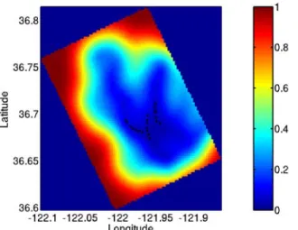
The maps use measurements over a four-hour window centered on the time of the map (midnight UTC). The measurement locations for the two-hour span starting with the map time are plotted as black dots. For the gliders, each measurement corresponds to data collected during one yo of a glider. The
maps for the gliders are shown in Figures18and19. The error
map for the towfish with σ = 1.5 km is shown in Figure20.
The measurement locations for the towfish are the locations of the 25 meter depth crossings.
Fig. 18. Error map for gliders withσ = 1.5 km and τ = 1 day. August 16,
2003 demonstration.
Fig. 19. Error map for gliders withσ = 3.0 km and τ = 1 day. August 16,
2003 demonstration.
Note that σ determines the cross-track width of the sensor
swath. At 3 km spacing of the glider formation, the root-mean-square estimate error at the center of the glider formation is
0.2 forσ = 3 km and 0.05 for σ = 1.5 km. According to this
metric, the triangle formation with 3 km spacing gives very good error reduction at its centroid when the spatial scale is
defined by σ = 3 km (and the temporal scale by τ = 1 day)
and truly excellent accuracy in estimation of the process along
the path of its centroid when σ = 1.5 km.
Fig. 20. Error map for towfish withσ = 1.5 km and τ = 1 day. August
16, 2003 demonstration.
Similarly, γ, defined by τ /σ times the vehicle speed,
determines the along-track length of the sensor swath. The
effectiveγ is about 10 for the gliders, 30 for the Dorado and
300 for the towfish atσ = 3 km and τ = 1 day. Choosing the
best towfish track for sampling is most like the “lawnmower” problem.
For these values of σ and γ, the glider formation
orien-tation accuracy is more important than inter-vehicle spacing accuracy. Orientation accuracy (to ensure maximum trackline separation) will enlarge the array sampling footprint by reduc-ing overlappreduc-ing sensor swaths.
C. Aug 23, 2003 Drifter Tracking
In this sea trial we controlled a Slocum glider to follow a Lagrangian drifter in real time. This sea trial was meant to demonstrate the utility of the glider to track Lagrangian particle features such as a water mass encompassing an algae bloom.
During the experiment the drifter transmitted its position data approximately every 30 minutes. The data arrived at the command station with a 15 minute lag. In order to follow the drifter in real time it was necessary to predict the future trajectory of the drifter. This prediction was based on a persistence rule, using a quadratic or a linear curve fit of measured positions and corresponding time stamps.
The persistence rule was used to estimate
1) The position of the drifter at the next estimated surfacing
time of the glider.
2) The average velocity of the drifter during the following
glider dive cycle.
The above information was used in conjunction with the estimated surfacing location of the glider (calculated using the glider estimator described in§III-B) to determine the glider waypoint list. The glider surfaced approximately every 2 hours as in the demonstrations described above.
The goal of this demonstration was to have the glider travel back and forth along a chord of a circle (of specified radius)
with respect to the drifter, as shown in Fig. 21.
Fig. 21. Drifter Tracking Plan: The solid circles indicate drifter positions at two time instants, and the line connecting the solid circles is the drifter path. The solid line crossing the drifter path is the desired glider path. The glider path with respect to the drifter is a chord of a circle of specified radius about the drifter.
Fig.22shows the actual tracks followed by the drifter and
the glider during the demonstration.
The estimated currents onboard the glider and the currents experienced by the drifter were significantly different. This is indicative of a three-dimensional flow structure, which the glider had to negotiate. The drifter, on the other hand, was affected only by the surface currents.
Moreover, since the glider surfaced only every two hours, its waypoints were based on a two-hour estimation of drifter trajectory. This estimation was not so accurate since the drifter trajectory did not persist that long.
The average speed of the drifter during this demonstration was approximately 7 cm/s. Towards the end of the experiment the drifter moved much slower and its displacement in half an hour was less than the GPS measurement scale. As a result the drifter appeared stationary on the GPS scale.
The glider caught up with the drifter quickly, but unknown velocity fields, time delays in the control implementation and the limited sensitivity of the GPS contributed to errors in tracking. Additionally a bug in the waypoint calculation code also introduced errors in the first few dive cycles of the experiment.
In order to improve the accuracy of drifter tracking one could modify this approach slightly to follow the path traced by the drifter a posteriori instead of estimating and tracking the future trajectory of the drifter. This way the glider would be able to cross the drifter path several times. The frequency and amplitude of cross-path swaths of the glider could be adjusted based on the drifter speed. This strategy induces a tracking time delay on the order of the glider surfacing period, which was two hours for our demonstration. Such a time delay may
−121.94 −121.92 −121.9 36.82 36.84 36.86 36.88 A Latitude Longitude Glider Drifter −121.924 −121.92 −121.916 −121.912 36.864 36.868 36.872 36.876 36.88 B
Fig. 22. Tracks followed by the glider and the drifter during the August 23, 2003 demonstration. (A) The complete demonstration. (B) The last four glider dive cycles - the dashed line is the drifter track and the solid line is the glider track. The color of the solid line changes at the start of every new dive.
be acceptable, especially since the tracking accuracy will be greatly improved.
V. FINALREMARKS
We have described a method for cooperative control of multiple vehicles that enables adaptable formation control and missions such as gradient climbing in a sampled environment. This method has been implemented on a fleet of autonomous underwater gliders which have high endurance but move slowly and are sensitive to currents. Results are described from several sea trials performed in August 2003 in Monterey Bay. These results show that groups of AUV’s, namely gliders, can be controlled as formations which move around as required, maintaining prescribed formation orientation and inter-vehicle spacing with decent accuracy despite periods of strong currents and numerous operational constraints.
Temperature gradient estimates computed from on-board glider temperature measurements taken during these sea trials are shown to be smooth and at least qualitatively well cor-related with temperature fields measured by satellite. These results suggest good potential for cooperative formation con-trol in gradient climbing and feature tracking for physical and biological processes.
Feature tracking can contribute to adaptive ocean sampling strategies, especially for estimating processes at smaller scales. As part of the analysis of the August 16, 2003 demonstration, we examined the capability of the glider groups and other mo-bile sensor platforms to sample for the purpose of minimizing estimation error of a process of interest given a priori statistics for the process. A metric based on this objective analysis error
can be used to judge sampling performance for a sensor array. This metric, which looks at minimization of estimation error, is directly related to maximization of entropic information.
This metric can also be used to derive optimal sensor array designs. In current work, we are examining optimal sensor array designs for vehicle groups in broad-area coverage prob-lems using this and related metrics. We are also developing alternative cooperative control strategies well-suited to the broad-area coverage problem, see, for example, [13]. Sea trials are planned for 2006 as part of the Adaptive Sampling and Prediction project [1].
VI. ACKNOWLEDGEMENTS
We gratefully acknowledge all of the other AOSN team members for support, collaboration and easy access to relevant data. We are especially grateful to Steve Haddock and John Ryan for their help with the Dorado and the towfish in the cooperative, multi-vehicle demonstration on August 16, 2003 and Francisco Chavez for his help with the drifter for the demonstration on August 23, 2003.
REFERENCES
[1] Adaptive sampling and prediction (ASAP), collaborative MURI project. http://www.princeton.edu/˜dcsl/asap.
[2] Autonomous ocean sampling network (AOSN) II, collaborative project. http://www.princeton.edu/˜dcsl/aosn.
[3] F.P. Bretherton, R.E. Davis, and C.B. Fandry. A technique for objective analysis and design of oceanographic experiments applied to MODE-73.
Deep-Sea Research, 23:559–582, 1976.
[4] C. C. Eriksen, T. J. Osse, T. Light, R. D. Wen, T. W. Lehmann, P. L. Sabin, J. W. Ballard, and A. M. Chiodi. Seaglider: A long range autonomous underwater vehicle for oceanographic research. IEEE
Journal of Oceanic Engineering, 26(4):424–436, 2001. Special Issue on
Autonomous Ocean-Sampling Networks.
[5] E. Fiorelli, P. Bhatta, N.E. Leonard, and I. Shulman. Adaptive sampling using feedback control of an autonomous underwater glider fleet. In
Proc. of Symposium on Unmanned Utethered Submersible Technology,
2003.
[6] V. Kumar, N. E. Leonard, and A. S. Morse, editors. Proceedings of the
Block Island Workshop on Cooperative Control. Springer-Verlag, New
York, 2004. In press.
[7] N.E. Leonard and E. Fiorelli. Virtual leaders, artificial potentials and coordinated control of groups. In Proc. 40th IEEE Conf. Decision and
Control, pages 2968–2973, 2001.
[8] P. F. J. Lermusiaux. Data assimilation via error subspace statistical estimation, partII: Mid-Atlantic bight shelfbreak front simulations, and ESSE validation. Montly Weather Review, 127(8):1408–1432, 1999. [9] P. ¨Ogren, E. Fiorelli, and N. E. Leonard. Cooperative control of
mobile sensor networks: Adaptive gradient climbing in a distributed environment. IEEE Trans. Automatic Control, August 2004.
[10] P. ¨Ogren, E. Fiorelli, and N.E. Leonard. Formations with a mission: Stable coordination of vehicle group maneuvers. In Proc. Symposium
of Mathematical Theory of Networks and Systems, 2002.
[11] D. L. Rudnick, R. E. Davis, C. C. Eriksen, D. M. Fratantoni, and M. J. Perry. Underwater gliders for ocean research. In press, 2004. [12] B. Schultz, B. Hobson, M. Kemp, J. Meyer, R. Moody, H. Pinnix, and
M. St. Clair. Multi-UUV missions using RANGER MicroUUVs. In
Proc. Unmanned Untethered Submersible Tech., 2003.
[13] R. Sepulchre, D. Paley, and N. Leonard. Collective motion and oscillator synchronization. In V.J. Kumar, N.E. Leonard, and A.S. Morse, editors, To appear in Proc. Block Island Workshop on Cooperative Control, June 2003.
[14] J. Sherman, R. E. Davis, W. B. Owens, and J. Valdes. The autonomous underwater glider ‘Spray’. IEEE Journal of Oceanic Engineering,
26(4):437–446, 2001. Special Issue on Autonomous Ocean-Sampling Networks.
[15] D. C. Webb, P. J. Simonetti, and C.P. Jones. SLOCUM: An underwater glider propelled by environmental energy. IEEE Journal of Oceanic
Engineering, 26(4):447–452, 2001. Special Issue on Autonomous Ocean-Sampling Networks.