Amplitude fluctuation effects in shallow water acoustic scattering by internal waves

Amplitude Fluctuation Effects in Shallow Water

Acous-tic Scattering by Internal Waves

by Lei Fu

B.S., Peking University, P. R. China (1990)

M.S., The Chinese Academy of Sciences, P. R. China (1993) Submitted in partial fulfillment of the requirements for the degree of

MASTER OF SCIENCE IN OCEANOGRAPHIC ENGINEERING at the

MASSACHUSETTS INSTITUTE OF TECHNOLOGY and the

WOODS HOLE OCEANOGRAPHIC INSTITUTION August 1995

Copyright 1995, Lei Fu. All rights reserved.

The author hereby grants to MIT and WHOI permission to reproduce and to distribute copies of this thesis docunAent in whole or in part.

A uthor... ... ... MIT/WHOI Joint Program in Oceanographic Engineering C ertified by ... ... "'"'"'"'"'"'""'"""'"'"'"'""'"'"'"'"'""'"...

S.Dr. James Lynch

Associateci t, Woods Hole Oceanographic Institution Thesis Supervisor C ertified by... ... . ...

Professor Henrik Schmidt Professor of Ocean Engineering, Massachusetts Institute of Technology Thesis Reader Accepted by... ... . ... ... ... . ...

Profe sor Arthur B. Baggereor Chairman, MIT/WHOI Joint Committee of Oceanographic Engineering

.. ¢SACH.US -IFT. INSr;i"-UTL OF TECHN(L.OGY

DEC 0 8

1995

Amplitude Fluctuation Effects in Shallow Water

Acous-tic Scattering by Internal Waves

by Lei Fu

Submitted to MIT/WHOI Joint Program in Oceanographic Engi-neering in partial fulfillment of the requirements for the degree of

Master of Science in Oceanographic Engineering

Abstract

This thesis investigates the amplitude fluctuation effects in acoustic scattering due to shal-low water internal waves. Theoretically, it uses the adiabatic approximation and perturba-tion methods to statistically evaluate acoustic transmission fluctuaperturba-tions caused by internal waves in the ocean; it also investigates acoustic mode coupling effect due to internal waves. Numerically, this thesis simulates the shallow water internal wave(IW) field using the Garrett-Munk internal wave spectrum model and then evaluates acoustic transmission in the simulated internal wave field with the Kraken normal mode program. Theoretical calculations are also performed using the theory developed in this thesis. Comparisons are made between theory and numerical calculations.

The results presented and discussed in this thesis are related to the following issues: coher-ent and incohercoher-ent intensity fluctuations for adiabatic approximation, acoustic mode cou-pling due to IW's, transmission loss difference between adiabatic and coupled mode methods, and their dependence on range, IW amplitude and frequency.

Thesis Supervisor: Dr. James Lynch

Acknowledgments

First of all, I would like to thank my thesis supervisor, Dr. James Lynch, for giving me motivation, encouragement, guidance, and help all the time during my graduate study in the MIT/WHOI joint program. He even read and edited every sentence in my thesis draft. All in all, I would like to say: thank you very much, Jim!

I would also like to thank Professor Henrik Schmidt for reading my thesis and giving me his comments from an expert point of view. I thank Professor Arthur Baggeroer, my academic advisor at MIT, for advising me on my academic study in the Joint Program.

I thank Arthur Newhall for helping me on computer work in general and on the Kraken program in particular. I also thank Peter Traykovski for giving me his IW mode codes and Michael Porter for allowing me to use two of his figures in my thesis.

Dezhang Chu and Dajun Tang offered me much help during my study at WHOI. I thank them for their help and sincerity.

Thanks also go to John Farrington, Jake Peirson, Abbie Calvin, Ronni Schwartz, and all other WHOI Education Office staff for their support of my study in the Joint Program.

My fellow students and friends at WHOI and MIT have been always a source of help, information and fun. I thank them for their help and the wonderful time we had together.

Finally, I especially thank my wife, Zhaohui and all of my family, my grandparents, my parents, my brother and my sister for their love, support, and understanding.

Table of contents

Abstract

2

Acknowledgments

3

List of Tables

7

List of Figures

8

1. Introduction

11

1.2 Thesis objectives and organization 12

2. Internal waves in the ocean

14

2.1 Introduction 14

2.2 Theory 14

2.3 Experimental measurement of internal waves 17

2.4 Garrett-Munk internal wave model 19

2.5 Solitons (solitary internal waves) 21

3. Acoustic scattering due to internal waves

23

3.1 Normal mode theory 23

3.2 Adiabatic approximation 27

3.3 Adiabatic description of acoustic scattering due to internal waves 31 3.4 Coupled mode description of acoustic scattering due to internal waves 42

3.5 Solitons vs. linear internal waves 48

4. Simulations and numerical calculations

51

4.1 Realization of Garrett-Munk internal wave field 51

4.2 Acoustic waveguide model 55

4.3 The KRAKEN normal mode program 61

5.

Conclusions and Future work

5.2 Recommendations for future work

Appendix A

Calculations of eigenvalue and eigenfunction perturbations

References

94

97

List of tables

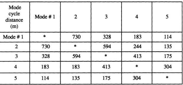
4.1 Horizontal wavenumbers and mode amplitudes for the background sound speed profile with frequency of 100Hz and source depth of 30m... ... 58 4.2 Mode cycle distance between each pair of acoustic modes for the background sound speed profile with frequency of 100Hz...58 4.3 Horizontal wavenumbers and mode amplitudes for the background sound speed profile with frequency of 50Hz and source depth of 30m... .... 72 4.4 Mode cycle distance between each pair of acoustic modes for the background sound speed profile with frequency of 50Hz... ... 72 4.5 Horizontal wavenumbers and mode amplitudes for the background sound speed profile with frequency of 200Hz and source depth of 30m... ... 73 4.6 Mode cycle distance between each pair of acoustic modes for the background sound speed profile with frequency of 200Hz...74

List of figures:

4.1 (a) Buoyancy frequency profile N(z); (b) Internal wave modes calculated from

E q.(2.16) ... 52

4.2 Garrett-Munk IW spectrum used for simulating the IW field...53

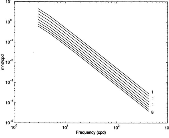
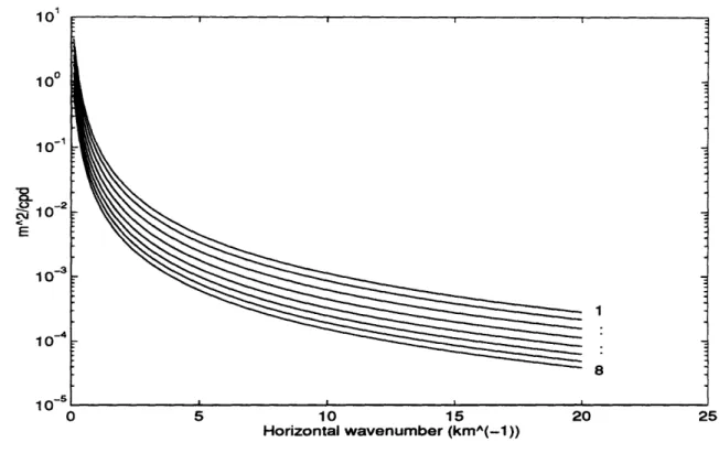
4.3 IW horizontal wavenumber spectrum for modes 1-8...54

4.4 One realization of IW vertical displacement from GM spectrum...54

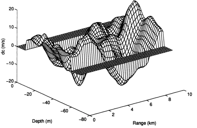
4.5 One realization of IW induced sound speed fluctuations rom GM spectrum...55

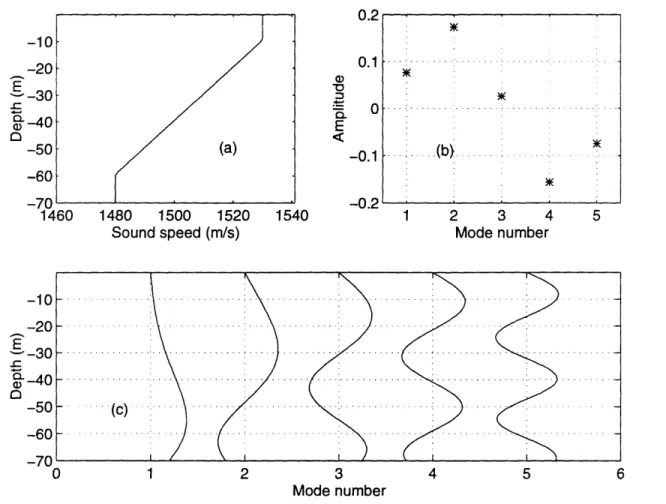
4.6 (a) Background sound speed profile; (b) mode amplitudes for source depth of 30m; (c) acoustic modes calculated using Kraken programs. Frequency = 100Hz...57

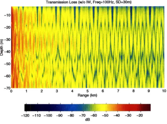
4.7 2-D transmission loss for the background sound speed profile model with fre-quency of 100Hz and source depth of 30m... ... 59

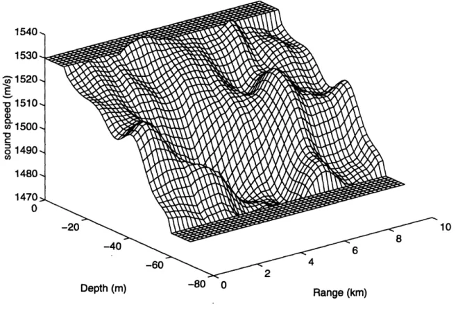
4.8 One realization of sound speed profiles with IW induced fluctuations...60

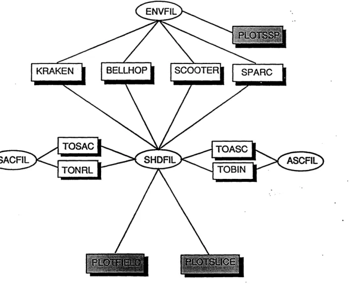
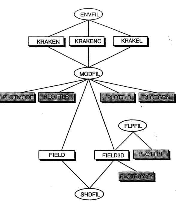
4.9 Structure of the Acoustics Toolbox... 63

4.10 Structure of the KRAKEN model ... 64

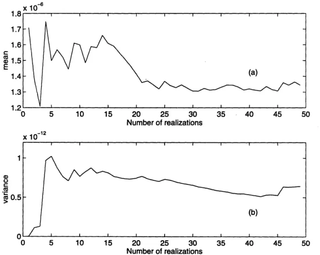
4.11 Mean and variance of acoustic intensity vs. number of realizations at range of 5km and receiver depth of 30m. Frequency = 100Hz...66

4.12 Transmission loss at receiver depth of 30m for frequency of 100Hz and source depth of 30m ... ... 75

4.13 Standard deviation normalized by mean value for the acoustic intensity from adi-abatic calculation. IW amplitude = 10m and frequency = 100Hz...75

4.14 Standard deviation normalized by mean value for the acoustic intensity from cou-pled mode calculation. IW amplitude = 10m and acoustic frequency = 100Hz...76

4.15 Transmission loss difference between adiabatic approximation and coupled mode calculations (average of 49 realizations). Frequency = 100Hz... 76

4.16 Transmission loss difference between adiabatic approximation and coupled mode calculations. Frequency = 100Hz, source depth = 30m, and receiver depth = 10m...77 4.17 Acoustic horizontal wavenumber perturbations vs. range for one realization of IW induced sound speed fluctuations. Frequency = 100 Hz...78

4.18 Modal phase perturbations vs. range due to the horizontal wavenumber perturba-tions show n in Fig. 4.17 ... 79 4.19 TL difference between adiabatic approximation and coupled mode calculations (average of 49 realizations) for frequency of 100Hz and IW amplitude of 20m...80 4.20 TL difference between adiabatic approximation and coupled mode calculations (average of 49 realizations) for frequency of 100Hz and IW amplitude of 30m...80 4.21 TL difference between adiabatic and coupled mode calculations (average of 49 realizations) for IW amplitude of 10m, 20m, 30m at receiver depth of 10m and 30m...81 4.22 The average ratio of standard deviation to mean value of coherent intensity for different amplitudes. Frequency = 100Hz... 82

4.23 TL difference between adiabatic and coupled mode calculations (average of 49 realizations) for frequency of 50Hz... 83 4.24 TL difference between adiabatic and coupled mode calculations (average of 49 realizations) for frequency of 200Hz... 83

4.25 TL difference between adiabatic and coupled mode calculations (average of 49 realizations) for different frequencies at receiver depth of 10m and 30m...84

4.26 The average ratio of standard deviation to mean value of coherent intensity for different frequencies at different receiver depths. IW amplitude and source depth are the

sam e...85

4.27 Coherent and incoherent transmission loss curves at receiver depth of 30m for IW amplitude of 20m, frequency of 100Hz and source depth of 30m... 88

4.28 Coherent and incoherent transmission loss curves at receiver depth of 30m for IW amplitude of 30m, frequency of 100Hz, and source depth of 30m... 88

4.29 The ratio (average of 49 realizations) of standard deviation to mean value of inco-herent intensity (Kraken results). Frequency = 100Hz, IW amplitude = 20m, and source depth = 30m ... ... 89 4.30 The ratio (average of 49 realizations) of standard deviation to mean value for incoherent intensity (theoretical results). Frequency = 100Hz, IW amplitude = 20m, and

source depth = 30m ... ... 89 4.31 The average ratio of standard deviation to mean value of incoherent intensity (Kraken results) vs. IW amplitude at different depths...90

Chapter 1

Introduction

1.1 Background

Sound waves, with much lower attenuation than electromagnetic waves in water, can propagate very long distances in the ocean and thus have been utilized in many military and civilian applications, such as sonar systems, underwater communication, ocean explo-ration, etc. Spurred on by the usefulness of underwater sound, researchers have been mak-ing progress in every area of ocean acoustics. An acoustical signal received at a point in the ocean from a remote source can vary considerably in amplitude, travel time, and even the direction from which it arrives because of inhomogeneities and fluctuations in the ocean environment. These effects might seriously degrade the performance of sonar sys-tems and many other underwater applications. However, one man's noise could be another's signal. The acoustic fluctuations also may provide us a valuable way to explore the ocean. Thus research into acoustic fluctuations due to various oceanic processes has been drawing much effort[ 1][2]. The process that this thesis will concentrate on is internal waves in the ocean.

Internal waves(IW's) are similar to ordinary sea surface waves except that they occur within the sea rather than at the surface. They exist at interfaces between water layers of different density, especially at the pycnocline. In a homogeneous sea, they can not exist. Internal waves characteristically have greater amplitudes and slower speeds of propaga-tion than do surface waves. Internal wave induced sound speed fluctuapropaga-tions cause acoustic scattering when sound waves propagate through a water column with internal wave activ-ity.

Much of the work on acoustic scattering by internal waves has been concerned with the deep ocean. In a book edited by Flatte [1], a clear overview is given of the work in this area up until 1979. There was also theoretical work on the statistics of normal mode amplitudes in the internal wave field by Dozier and Tappert [3][4]. As for the work on acoustic scattering by shallow water internal waves, some highlights are the study of reso-nant acoustic scattering by internal wave solitons by Zhou, Zhang, and Rogers[5], the study of acoustic modal wavenumber fluctuations by Essen[6], and the studies of internal wave induced phase front curvature across horizontal arrays by Shmelerv[7], Ruben-stein[8], and their co-workers. The first Zhou et al study concentrated on acoustic ampli-tude attenuation effect, and the latter two studies focused on phase fluctuations. In recent work by Lynch et al.[9] and Traykovski[ 10], acoustic travel time perturbations due to shal-low water internal waves and internal tides in the Barents Sea Polar Front have been stud-ied.

1.2 Thesis objectives and organization

In this thesis, we will investigate the amplitude fluctuation effects in acoustic scattering due to linear shallow water internal waves. We mainly use adiabatic approximation method to describe "weak scattering" due to linear internal waves. We will also look at mode coupling effect and compare acoustic scattering by linear internal waves with that by solitons. The main argument we would like to make is that for linear internal waves, when the mode cycle distances are much less than the "dominant" 1W wavelength, the coupling is small and the adiabatic approximation is valid.

This thesis is organized as follows. Chapter 1 is the introduction. Chapter 2 is about internal waves in the ocean: theory, observation techniques, data analysis, the Garrett-Munk(GM) model, and solitons. Chapter 3 is the main theoretical part of this thesis in which we develop the full theory for coherent and incoherent intensity fluctuations due to internal waves and describe the resonant coupling effect. Chapter 4 contains simulations and numerical calculations; specifically we make simulations of the Garrett-Munk IW model, use the Kraken normal mode program to evaluate the acoustic field in the simu-lated internal wave environment, do calculations using the theories developed in Chapter 3, and then discuss the results. We present conclusions in Chapter 5.

Chapter 1 and 2 are generally a review of previous work. Chapters 3-5 are mainly my own contributions.

Chapter 2

Internal waves in the ocean

2.1 Introduction

Internal waves occur beneath the sea surface between water layers of different density. These gravity waves propagate along a pycnocline associated with either a halocline or thermocline. The causes of internal waves are varied and not completely understood. Some causes are: flow over bathymetry, storms, surface waves, tidal action, wind blowing over the sea surface, etc. Internal waves travel more slowly than surface waves, but can attain much greater amplitudes. They mix water below the surface and may be important in the movement of sediments.

Internal waves can be found in both shallow and deep ocean water and in large fresh-water lakes, such as Lake Ontario. "Typical" characteristics of internal waves are as fol-lows[11]: in shallow water, the internal waves have periods of 4 minutes to 25 hours, amplitudes of up to 20m, and speeds of order of 5 cm/sec; in deep ocean, the internal waves have periods of 4 minutes to 25 hours, amplitudes of up to 100 m, and speeds of

100 cm/sec.

2.2 Theory

Using the basic equations of momentum and continuity for a fluid, an exact modal solution for internal waves can be derived. The momentum equation for an isotropic fluid in the absence of viscous effect is given by [12]

+ 2rlx' = -p-'V p-' (2.1)

and the continuity equation for an incompressible fluid is given by

au av aw

Ve U + +z + = 0 (2.2)

Applying small perturbation terms p' and p', the perturbed pressure and density are then given respectively by

p = -gpz+p' (2.3)

p = po+ p' (2.4)

Substituting Eqs. (2.3) and (2.4) into Eq. (2.1), the momentum equation is then linearized by neglecting the high order perturbation terms, i.e. products of perturbation quantities, and becomes au _{-fv --} 1 ap' _(2.5)

at

Poax

at

poay

1

ap'

where f is the inertial or "local Coriolis" frequency. We now assume a separable solution for the vertical velocity w (x) of the form

w (, t) = i (z) exp [i (kx + ly - Ot) ] (2.8)

The vertical velocity w (1) satisfies the boundary conditions of no normal flow at the bot-tom, i.e.

and that a particle on the free surface remains on it

w (k) = at z = r (surface) (2.10)

which can be applied at z = 0 since rn is small. This approximation introduces little error since the vertical displacement at the air-water interface is smaller than the maximum amplitude by about 1000. By manipulating equations (2.3-2.8), we can obtain

a

_+

k

(Z)

-

=

0

aZ2 (02 ol (2.11)

where kh is the horizontal wavenumber that satisfies

k2 = k2+ 12 (2.12)

and where N (z) is the buoyancy frequency which is defined as

N

g dp

Podz (2.13)

The propagating wave solution for Eq. (2.11) only exits when f< o <N. Using the relation-ship

(2.14)

at

where 4 is the vertical particle displacement, and substituting it into Eq.(2. 11) gives

i9 V_8 N2 =2-

0

at•-(kh

Z _

2

0

=

with the following boundary conditions:

(z) = 0 at z = 0 (surface) (2.16)

and

• (z) = 0 at z = H (bottom). (2.17)

This equation can be formulated as an eigenvalue equation and is easily solved using numerical methods such as finite element methods. The exact modal solution is

= • ,(z) exp [i(kxtx+ky - Ot) ] (2.18)

i=

where 1 = 1, 2, ... is the mode number, At is the amplitude, and 0, (z) is the internal wave mode eigenfunction. In cylindrical coordinates, Eq.(2.18) can be expressed as

S(r, z) = Al (kr, o) 1(z) exp [i(krr-ot)] (2.19)

i= 1

where kr is the horizontal wavenumber.

2.3 Experimental measurement of internal waves

A variety of observational techniques are now available to measure internal waves in the ocean. Among them are moored sensors, towed sensors, dropped instruments[13], and remote sensing[14][15]. Also, because internal wave-induced variations in sound speed has strong effects on acoustical signal fluctuations, acoustic transmission measurement can provide a measure of certain statistical properties of the internal wave field[6][16].

Current meters, temperature sensors, and vertical temperature gradient sensors, which are attached to a more or less vertical mooring line between an anchor on the seafloor and a buoyant float at or below the sea surface, provide time series of current speed and direc-tion, temperature fluctuations, and vertical temperature gradient which give us temporal measurements of the ocean process. Usually a number of sensors are used at different ver-tical spacings on the same mooring, or on several moorings separated by various distances horizontally. The relationships between simultaneous measurements at different places provide the spatial information on the ocean processes.

A thermistor chain, consisting of a cable with sensors every a few meters, can be sus-pended below a ship and towed slowly through the upper layer of the ocean, mapping out a two-dimensional section of temperature structure down to about 200m below the sur-face.

Instruments lowered from a hove-to vessel, or dropped freely, are very traditional ways to measure the vertical structure of the oceans. The XBT (expendable bathythermo-graph) can be dropped from a ship to measure the temperature profile. The CTD (conduc-tivity, temperature, depth) records electrical conductivity and temperature (and hence salinity and density) as functions of depth as it is lowered from a stationary ship.

Remote sensing images from aircraft and satellites provide another way to observe the internal waves in the ocean. A nice example is the signatures of internal waves which were detected repeatedly in the Gulf of California by the Seasat synthetic aperture radar(SAR) [15].

Given a series of data points obtained from various instruments, which bear the tempo-ral and spatial information, the problem then is how to interpret them, i.e. how to relate them to internal waves. A basic tool in the interpretation of a series of data points is the

power spectrum. A time series can be related to a frequency spectrum and a spatial data series can be related to a wavenumber spectrum.

2.4 Garrett-Munk internal wave model

Based on experimental data on power spectra and cross spectra from many different sources, together with some simplifying assumptions, Garrett and Munk came up with a simple model describing the deep ocean distribution of internal wave energy in wavenum-ber-frequency space. The description of the model is as follows [17].

All quantities are nondimensionalized with reference to the deep ocean buoyancy scale depth b(1.3 km) and the buoyancy frequency no (3 cph) at the top of the thermocline.

Horizontal wavenumber a (a,, a2) and vertical wavenumber P are related to the mode

number j(1,2,...) and frequency Co according to the approximate formulas

oa = ja (02 -_f2) 1/2 (2.20)

P = jtN(z) (2.21)

where f is the inertial frequency and N (z) is the buoyancy frequency. If horizontal isot-ropy is assumed, various forms of the energy spectrum are related according to

JJE (a,1 a2,

)

1)

= E (a, o) dado = fJE(0, o) dpdao = E (2.22)

where E is a dimensionless constant related to the IW energy per unit area. With this and the dispersion relations, we can make transformations into various frequency-wavenum-ber spaces. The mode numfrequency-wavenum-ber scale j. and associated wavenumfrequency-wavenum-bers are

a, = j 7 (c02 2)1/ 2_{, p. = j.7N (z), j. = 6}

Most of the energy is contained in wavenumbers less than a, and P* according to

A (k) = (t- 1) (1 +X) -', X = a/a, = P3/P, t = 2.5 (2.24)

Further, set

B (w) = 27-r'fo-2'f , y = (1 - /02) 1/2 (2.25)

for f< W < N (z) , and zero otherwise. The functions A and B are so normalized that

oA (k)dX = 1, oB (o) do = I (2.26)

With all the above definitions and assumptions, the energy spectrum is specified as

E (a, o) = EA (a/a,)B( (m)/a., E = 6.3 x 10-5 (2.27)

This includes the similarity assumption that the shape of the spectrum as a function of hor-izontal wavenumber is invariant but for a scale factor, a,. Following the rules for transfor-mation, we obtain E (0, o) = EA (0/0,) B (C)/ /, 2x-'fEN(z) (0/0,) A (0/3,) E(a, ) = N2 (z) a2 +a 2 0 a• 0 [1 -/N 2 (z) ] 1/2 (2.28) (2.29)

The frequency spectrum is simply

E (co) = E (a, co) da.

(2.23)

2.5 Solitons(solitary internal waves)

Solitons (solitary internal waves) are discrete non-dispersive packets of internal waves which are of much shorter wavelength and larger velocity than the usual linear internal waves. Solitons have been observed in many coastal zones of the world such as[5]: Massa-chusetts Bay, the New York Bight, the Gulf of California, the Andaman Sea offshore Thai-land, the Australian North West Shelf, the Sulu Sea between the Philippines and Borneo, off the coast of Portugal, off the Hainan Island in the South China Sea, off the Strait of Gibraltar in the Alboran Sea, the Scotian Shelf off Nova Acotis, the Celtic Sea, and so on. The experimental data on them includes: current and temperature measurements, vertical profiles from CTD, XBT, and acoustic echo sounding devices, and radar and satellite images.

The generation mechanism of solitary internal waves (SIW) has long been a research area in the geophysics and fluid mechanics communities[18]. In shelf regions, stratifica-tion often has a pronounced two-layer character and a thermocline (i.e the interface between water layers with different temperatures) is established. The most non-linear hydrodynamic process occurring in a shelf thermocline is a bore, which is a stepwise vari-ation of the thermocline level which is often accompanied by large-amplitude oscillvari-ations. Bores usually generates intense pulselike short-period waves which may be associated with soliton formation. The Korteweg-deVries (K-dV) equation models the transformation of a bore as the decomposition of a stepwise perturbation into a sequence of solitons. In the coastal seas connected to the open ocean, some experiments show that solitons are caused by the transformation of barotropic semidiurnal tides into baroclinic motions. Internal tide solitons occur when tidal excursions are greater than or equal to the

topo-graphic length scale or when the Froude number is greater than or equal to 1(tidal current speed >internal wave speed).

Recent experiments suggest that SIWs are rather typical elements of internal motions, not only in the shelf zone but also in deep waters, at least up to hundreds of kilometers from the shelf. The observations of SIW in the deep ocean have been reported by many researchers[18]. The available data show that the SIW may appear both on the seasonal and on the main, permanent pycnoclines.

The main cause of the generation of SIWs in the ocean is the semidiurnal tide. And this phenomenon is a typical final result of the transformation of barotropic tides into baroclinic motions. The adequate theoretical description of this problem is still open in

many cases because of the lack of hydrographic data. However, we can expect significant advances in this area because of more and more advanced experimental schemes.

Chapter 3

Acoustic scattering due to internal waves

3.1 Normal mode theory

The formal derivation of ocean acoustics normal mode theory can be found in many books about propagation.[19] Here we will briefly go through the derivation of normal mode theory for the case of point source in a cylindrical geometry to provide the founda-tion for later theoretical work. The derivafounda-tions in Sec. 3.1 and Sec. 3.2 mainly follow the book by Jensen et al. [20].

We begin with the Helmholtz equation in two dimensional space with sound speed and density depending only on depth z:

la ap a 1 ap o+ 2 s(r)8(z-zs)

(rt) +p(z) Z+ 2 ( ) p = (3.1)

rar ar (z) az cz (z) 2nr

Using the technique of separation of variables, we seek a solution of the unforced equation in the form of p (r, z) = 0 (r) Y (z). After substituting into the above equation and dividing through by o (r) v (z) , we find

dr

r _{+ p} (z ) ) + _

'

dr _{dz P ( z c}2

(z)j

The contents in the square brackets are functions of r and z respectively. Thus, the only way the equation can be satisfied is if each component is equal to a constant. Denoting this separation constant by k2,, we obtain the modal equation,

p (z)

4

(

dz (z)]

(z =2

Tm

(Z)

(3.3)

L C2 (kWrm(Zmdz

with F(o) = 0o, =0.

dZ z=D

Here, T

m (z) denotes the particular function T (z) obtained with the separation constant krm. The boundary conditions imposed imply a pressure-release surface located at z=0 and a perfectly rigid bottom located at z=D. The modal equation is a classical Sturm-Liouville eigenvalue problem whose properties are well-known. (We assume for the moment that

p (z) and c (z) are real functions). The modes of such Sturm-Liouville problems are orthog-onal, i.e.

p (z) dz = 0 for m n _(3.4)

o p (z)

The solutions of the modal equation are arbitrary to a multiplicative constant as is eas-ily seen from Eq.(3.3). In order to simplify the results, we shall assume that the modes are normalized so that

2

'1

(z)

D

p(z-

Finally, the modes form a complete set, which means we can represent an arbitrary function as a sum of the normal modes. Thus we write the pressure as

p(rz) wm(Z) I= o•qm(r) (3.6)

II d (rd di(z)+ (r)) ,(r)

rdr dr m

M

=

8(r) 8 (z - z)

2ir (3.7)

The term in square brackets can be further simplified using the modal equation(3.3). This yields

i = I{

(3.8) 8 (r)8(z - z )

2ir

Next we apply the operation

J

(*) (z) dz (3.9)

to Eq.(3.7). Because of the orthogonality property given in Eq.(3.4), only the nth term in the sum remains, yielding

r

d

4

rdr dr n

rn n

This is a standard equation whose solution is given in terms of the Hankel functions as

n (r) = n (zs)H1,2₎ (krnr)

4 -P(z,-•) (3.11)

The choice of Ho') or H(2) is determined by the radiation condition stating that energy

should be radiating outward as r -- ,. Since we have suppressed a time dependence of the

form exp (-icot) , we shall take the Hankel function of the first kind. Putting this all together, we find that

2

(3.12)

p (r, z) 4m I (Zs) m (z) H( )(krmr) m=l

or, using the asymptotic approximation to the Hankel function,

p (r,

z) i -i/4 m~d s (Zik r

( z ,) F,-,n M S,(z ,) , ( z) e _

This is the expression for complex pressure field. Transmission loss is defined by

TL (r, z) = -201og p (r-, ) , whPoer(r 1) where (3.13) (3.14) (3.15) Po (r) = _{4xr ,}

is the pressure for the source in free space. Thus one may write

TL (r, z) = _{-201og p (z) (z)}

. (

m= I

eik. r

(3.16)

In some cases it is useful to calculate an incoherent transmission loss defined by

1r m J r 2

TL t ~z) ----201o g p-( .)

e

(z kr m

(3.17)

When comparing theory to measured data which has been averaged over frequency, one can often simulate the resulting smoothed transmission loss by an incoherent modal summation. Incoherent transmission loss is often appropriate for shallow-water problems,

where the modes are bottom-interacting. Since bottom properties are often poorly known, the detailed interference pattern predicted by a coherent transmission loss calculation is sometimes not useful.

3.2 Adiabatic approximation

In the last section, we derived the normal mode equations for the range-independent prob-lem. But the real ocean environment is always range-dependent. The goal of this thesis is to begin to explore the range-dependent problem introduced by internal waves. As we will see in the following, the range-dependence causes coupling, i.e. energy transferring between different modes. Numerically, one way to deal with range-dependent problems is to divide the range axis into a number of segments and approximate the field as range independent within each segment. The solution within a range-independent segment is constructed using the standard normal-mode solution and then the interface conditions (continuity of pressure and normal velocity) are used to "glue" the solutions together. This is called the step-wise coupled mode method. The coupled mode method is straightfor-ward but leads to a somewhat computationally intensive procedure. Thus the "adiabatic approximation" method was introduced, which simplifies the above coupled-mode prob-lem by ignoring (1) the backscattered component of the field and (2) coupling between different-order modes at the segment interfaces. This approximation was originally intro-duced by Pierce[21] based on analogous results for the Schrodinger equation. The deriva-tion here follows secderiva-tions of the textbook by Jensen et al[20]. To derive this approximation, we return to the Helmholtz equation in cylindrical coordinates,

+ P (z) -

(

)

Since the modes form a complete set, we can represent the solution at any range as a sum of "local modes". We therefore seek a solution of the range-dependent problem in the form

(3.19) p(r,z) = I m (r) m (r,z)

M

where Ym (r, z) are the local modes defined by

(r, z) (r, z) + -2 kr2m(r) m (r,z) = 0. (3.20)

Thus, at any range r,'m (r, z) is found by solving the depth-separated modal equation with the environmental properties at that range. Substituting into the Helmholtz equation yields

rc)r par(i m)) + m

(r) (r) 8 (z - ,) (r) mm = 271r

where we have used Eq.(3.20) to eliminate the z-derivatives. Rearranging terms leads to

am air T m m) ~z m t- •r ar + Pa raI'n +Xk 2 (r) ( T m (r) (z- ) 2cr

For simplicity, we now assume that p is independent of r. Then we apply the operator

S( r, z)

Jp (3.23)

and because of the orthogonality property, many of the terms in the sum will disappear.

a

ap

par ar

The result is

d

deD

dn

(r)

yT (Z,)

Note that Bmn = -Bnm, since differentiating

p (z) dz = Smn _(3.27)

P (z) mn'

gives

J

JFr p

p

Equations (3.24) is a statement of coupled modes written for the case of continuous variation of sound speed. It can be solved directly by, for instance, finite-differences. The adiabatic approximation can now be stated simply as the assumption that the coupling matrices Amn and Bmn are negligible. We then obtain a set of decoupled equations,

Id d 8 (r) n (zs)

d r-r n) + k n (r) D = 2ir (3.29)

rdr drn 2xr

which in the WKB approximation has the solution

iA J k,. (r') dr'

', (r) = (3.30)

·

The value of A is found by requiring that the WKB solutions match our standard solution, Eq.(3.13), when the problem is range-independent. Thus

A = P (z) i 8.7re i -ix/4 'n () (z.V) (3.31)(3.31)

By substituting this back to Eq.(3.13), we get the final result,

Sif kr (r') dr'

p (r, z) = e- 4 (zm ) ,, (r, z) e (3.32)

P (Z) r m=l

J

The problem with this expression is that it fails to satisfy reciprocity. So instead of using this expression, we use the following modified adiabatic formula:

if k,.rm (r') dr'

p (r, z) -= -m -i/4 () m (r z) (3.33)

p(z) m= ! okrm (r') dr'

This formula may be formally derived by assuming that the environment is invariant with respect to translations perpendicular to the radial connecting the source to the receiver. Having the above equation for pressure, we can now write the transmission loss expres-sion for adiabatic approximation:

TL (r, z) = -201og T (z) T' (r, z)

p (z)_ I

_m=1

TLInc (r, z) = -20log p n m (z5) m (r, z) 2 (3.35)

P(,) M=I

krm (r') dr'

3.3 Adiabatic description of acoustic scattering due to internal waves

Now we will use adiabatic approximation and perturbation methods to evaluate acous-tic scattering due to IW's. Whether the adiabaacous-tic approximation holds or not depends on the characteristics of the internal wave field. We will discuss the coupled mode description of the scattering by internal waves in Sec. 3.4 and the comparison between adiabatic and coupled mode methods in Sec 3.5.

From Eq.(3.33), the acoustic intensity can be written as

ii kr,.(r')dr' -J kn(r')dr I = A C m (Zs) m (r, z) n, (Zs) Tn (r, z) e (3.36) m n _{0 krm (r') 0' kr. V) dr'} where A - (3.37) 8Xrp 2 _(zs)

Rearranging the terms in Eq.(3.36), we obtain

•2 ( Zs) 2 ( r, z) I = Am Ya r m Jkrm (r') dr' i kr. (r') dr' - r k,, (r') dr ' +A T _m (Z.5) T m (r, z) T n (Zs) T n (r, z) e (3.38) mokrm _{(r') dr kr (r') dr'}

The first term in the right side of Eq.(3.38) is the incoherent intensity and the second term is the interference term. In this section, we will use the incoherent acoustic intensity and transmission loss to examine the acoustic scattering by the internal waves. We will also discuss the coherent intensity, which is the sum of the incoherent intensity and the interfer-ence term as in Eq.(3.38), and compare between coherent and incoherent intensities. There are three reasons why we choose to evaluate incoherent intensity and transmission loss. First, as I will also discuss later in this thesis, the internal wave -induced fluctuations are random so that the statistical mean of the coherent intensity approaches the incoherent

intensity under the condition of large variance. Secondly, as stated in the last section, for shallow water problems, the incoherent transmission loss is often appropriate since bottom properties are often poorly known, and hence the detailed interference pattern predicted by coherent transmission loss calculation is not always correct. Finally, it is easier to analyti-cally keep track of the derivations of the theoretical equations, so we start with the simple case first.

The incoherent acoustic intensity can be expressed as

0

im

(zs

Z)

_,()r,1Z)(3

linc = A

Y

M= f k rm ( r ) dr'

Next, we will use perturbation methods to evaluate linc. The perturbed sound speed is

c (r, z) = co (r, z) + Sc (r, z) (3.40)

where Bc (r, z) is the sound speed fluctuation, and c_o (r, z) is the background sound speed profile. 8c (r, z) is related to the internal waves by

where S, (r, z) = aco (r, z) is the sound speed gradient in the z direction and ý (r, z) is

vertical displacement in water column, which can be expressed as

(r, z) = a n (r) #n (r, z) (3.42)

n

where the d, (r, z) 's are the internal wave modes and the a, (r) 's are their amplitudes. The a, (r) 's are random variables whose mean and variance are

E (an) = 0 (3.43)

Var [an] = E [a ] (3.44)

From the above, we have

E[6c] = 0. (3.45)

Since 6c << co, we can use perturbation methods to evaluate the acoustic wavenumber

and mode function perturbations about the background. According to the paper by Rajan et al[22], the acoustic horizontal wavenumber perturbation due to sc is

.krm

(r) = Jo I k2 kPIo dz (3.46)

krm 0

where subscripts 0 and superscript (0) represent unperturbed terms. So we have

krm (r) =krm(0) + krm (r) (3.47)

Now we will find the mode function perturbations due to Sc, i.e. evaluate TI', (r, z) in

ym (r, z) = TY() (z) + STP (r, z). (3.48)

STYm (r, z) = amn (r) T(O) (z) ## e where 2ko8kY (0) To(0 ) dz amn(r) = (0)2 (0)2 rm rn (3.50)

Since k =-,then Sk = -- 8c. Substituting into Eq.(3.50)

C Co and then into Eq.(3.49) gives us

2ko c) (0) () dz c 2 0 o m 8'm (r,z) = n*m rm (0)2 -krn(0)2 a,(0) _(z) n (3.51)

Now we can expand Eq. (3.39) into

[~(' (0, z,) + 8Tm Mm (0 (O, z2 [) [ (r,2 r,) z) ) + "M Wt Sm(r, ,zZ)] 2

linc(r,z) = A

m=1 o [k +Skrm(r') Idr'

To the first order, this can be further simplified. For the mode perturbation terms,

[1T(' (0, z,) + 8) (0, z,) ] 2 (r, z) + SPm (r, z) ]2

= [ )2(0, zs) + 28m (0, zs) YI (0) (0, Zs)] [() 2 (r, z) + 28m (r, z) (0) (r, z) 1 (3.53)

= (O)2 (0, z,) (O) 2 (r, z) + 2S8n (0, z,) P () (0, Zs) (O)2 (r z) + 2(6m (r, z) () ( r, z) e(o)2 (0, z,)

And for the wavenumber perturbation term,

1 t[ k + Bkrm (r')] dr' Srm(0) (r') dr'

kr

+

Jo

_{(r') d}

Substituting Eq(3.53) and Eq(3.54) into Eq(3.52) and further simplifying it to first order gives us

linc (r, z) =

lin0)c

where

lo (r,z) =A( 1 I0)2 (0, z,) O)2 (r, z) (3.56)

m=l fk (r')dr'

is the intensity without any internal wave-induced perturbations, and

81')l (r, z) = A

5

is the intensity fluctuation due to mode shape perturbations, and

c 1r 8k rm

(r') dr'

81in2c (rz) =A r r()2 (0 z,) YT (O) 2 ( r, z ) (3.58)

m= I k0- (r')dr') dr' k (r ) dr

is the intensity fluctuation due to horizontal wavenumber perturbations.

From Eq.(3.46) and Eq.(3.51), the eigenvalue and eigenfunction perturbations are both caused by the internal wave-induced sound speed fluctuation and the mean value of the perturbation should be zero, i.e.

E [1•5I (r, z)] = 0 (3.59)

and

because of E [5c] = 0.

Before evaluating the variance, we first make some simplifications to Eq.(3.57) and Eq.(3.58). We assume that the background sound speed profile is range-independent. Then the eigenvalue k•' and eigenfunction '(y) (z) are range-independent. Thus Eq.(3.57) and Eq.(3.58) can be simplified to

•I(1) (r, z) SA r 28 . (0, z•) (, ) (z,) ()2 (z) + 26 . (r,z) Ti (°) (z) T ()2 )] (3.61) m = 1 rm r and 1 r Sk (r') dr' 81,() (r, z) = A Xo- Jo o()2 (z) (0)2 (z) (3.62) m = 1 krm r krm r

From Eq.(3.59) and Eq.(3.60), we know that

E [l,,c = li()c (3.63)

Then the variance of intensity is

8 (2)2 (2) (2) 2

Var [Ic]= E[ (E I ) (2) 2]= E[ (BIt))2] +2E [6S) S ] + E [ (51in) 2 (3.64)

Before we start evaluating the variance, let's examine Eqs. (3.61) and (3.62). In Eq.(3.62), we notice the l/r scaling factor which would cause 862I to fall off quickly with range with respect to 56

,lc.

on. Thus the only significant term on the right hand side of Eq.(3.64) is the first term which can be written as

1 - 2r''- 11 E 'IA ' [GLm+Jm ( [Gn +Jll] L k(

rm

n kOn

= A2' 1 _{1rk [E[GmG] +E[GmJ] +E [JmG,] +E[JmJ,]]} m _krm rn

E [GmGn] = 4T (0) (zs) T ( (z) I) (0)2 (Z) T(0) 2 (Z) E [S6 _m (0, z,) P, (0, zs) ]

E[GmJ] = 4Y (zs) T (Z) ozs (Z )2 (Z) T (0) 2 (Z0 ) E [6 8m (0, Zs) 6T (r, z)], E [JmG,] = 4•mO) (Z) T (o) (Zs) T (0) 2 (0)2 (z) E [ 8 m (r, z) 8, (0, zs) ]

E [JmJ] = 4 T) (Z) T (o) (Z) 0)2 (Z 0)2 )E [6m(r, s z) 6 (r, z)]

By substituting (3.51) into (3.69) - (3.72), we obtain

E [SY_m (0, z,) 8Y _n (0, z,) ] i 4kok'o SE [c (0, z) Sc (0, z-_{) ]} (0) ' (0) T (0) Tp (0) dzdz'

S(0)

JJ

coc

m

n

E [

B•Y

S'

4k 2k.,2 S

0 E [8c (r, z) Sc (0, z') ] qm(O) i(O) f/,(0) y (O)dzdz'

= (k0) 2_ (0)2) (k()2 - k(Z(0)

i*mj*n (k -k (k k 0)

and

E [ Ym (r, Z) •TYn (r, z)]

S" 0 0 oE[Sc (r, Z) Sc (r, Z')] y (O)t TpO) p (O) ,(0) dzdz' 0JJ CoC'o I i= *mj (0)2 (0) 2 ( 0)2 k (0r ) 2 (z)

rm

ri

r

ri

If we assume Sc is stationary over range and depth, we have

E [ec (r, z) c(r', z') ] = Rc (r - r', z -z') (3.77)

which is the autocorrelation function of 8c. With Eq.(3.41), we can reduce Eq.(3.77) to

E[Sc(r,z)Sc(r',z')] = SzS'E [4(r,z) (r',z')] = SzS'zRk(r-r',z-z') (3.78)

where Rý (r - r', z - z') is the 2-D autocorrelation function of vertical displacement 4. The autocorrelation function is related to the horizontal and vertical wavenumber spectrum Sg (kr, kz) by Fourier transform:

R4 (r, z) = f S (kr,kz) exp[ i (krr+kzz) ]dkrdkz. (3.79)

With Eqs. (3.68) - (3.79), we can evaluate the intensity variance in Eq.(3.64). Further-more, we assume that the 2-D correlation function can be factored into or at least approxi-mated by the product of horizontal autocorrelation function Rr (r) and vertical autocorrelation function R, (z) , i.e.

R (r,z) = R r(r) R4z(Z).

Substituting Eqs. (3.77), (3.78) and (3.80) into Eqs. (3.73)-(3.76) and manipulating the terms, we obtain

E [6• m(0, zs) 6n (0, zs)] = Rr (0) CEKmnij o' (z,) To) (zs) (3.81)

i mj n

E [m (0, zs) 8Tn (r, z) ] = Rtr(r) Kgmnijf TO) (Zs) I(O) (z) (3.82)

i*mj*n EI [Sm (r, z) 8Fn (0, Zs)] = R~,(r)

Y

T-7

oR°

z

(z-

z')

SS'zT(o

o) o)

T'(0)dzdz'

Eqs.(3.81)-(3.84) show that the horizontal structure of the incoherent intensity variance is determined by the autocorrelation function of the vertical displacement, i.e. Rtr (r) .

After finishing the incoherent intensity derivations, we now look at Eq.(3.38) to exam-ine coherent intensity. According to Eq.(3.38), the coherent intensity is the sum of the incoherent intensity and the interference terms. Thus the coherent intensity fluctuation is the sum of the incoherent intensity fluctuation and fluctuations of the interference terms. The interference term fluctuations are mainly caused by horizontally shifting of nulls in the interference structure of coherent intensity. We then need to determine the relative lev-els of the 'incoherent' fluctuations and 'interference' fluctuations. For the range-indepen-dent problem without any fluctuations, according to Eq.(3.38), we know that the

incoherent term and the interference term contribute to the coherent intensity at the same level. For the case of fluctuations, the incoherent fluctuations are first order perturbations which are much smaller than the unperturbed incoherent intensity according to the above derivations However, the interference fluctuations are basically caused by modal phase fluctuations. Due to phase wrapping effects, the phase fluctuations can have strong effect on the interference structure by causing nulls to shift back and forth, and hence the coher-ent intensity. Thus the interference intensity fluctuations are at the same level as the inter-ference intensity without fluctuations. With the above arguments, we can conclude that the coherent intensity fluctuations are mainly due to the interference fluctuations, i.e. the modal phase fluctuation. And then the horizontal structure, i.e. the range-dependence of the variance of the coherent intensity, is determined by the range-dependence of the vari-ance of the modal phase fluctuation.

We now investigate the variance of the phase fluctuations. The modal phase is

Pm = krm (r') dr' = k ) r + rkrm (r') dr' (3.86)

And the variance of the phase is thus

ar m] = E[8krm (r') dr' 6krm (r") dr" (3.87)

Substituting Eq.(3.46) into it, we find that

E1

1 E foc (r') 8c' (r")

dr'dr"]

Var[cpm] r

0 p-P

o

o2ol2k k'

CoC'o

dzdz'

Here the prime on the variable means that its argument is z'. Now we want to explore the range-dependence of the variance. Looking at the terms on the right side of Eq.(3.88), we

note that the range dependence is determined by the double integral

rr Sc (r') S c' (r'

) dr'dr" , i.e.

Var[pm] -E S5c (r') Sc' (r" ) dr'dr" (3.89)

Since the sound speed fluctuation 8c is related to the internal wave vertical displacement by Eq.(3.41), substituting it into Eq.(3.89) gives us

Var [Pm] -E[•: (r') (r") drdrdr" (3.90)

In the above step, we made some simplification by neglecting the depth dependence of 5. (this will not alter the qualitative results we will obtain shortly). We next consider an inter-nal wave at a single frequency. This doesn't lose generality because the spectrum can be decomposed into sinusoids by Fourier transform anyway. Thus we assume 4 (r) is a sto-chastic process which takes the form of

4(r) = cos(krr+O) (3.91)

where kr is the internal wave wavenumber and 0 is a random phase with uniform distribu-tion, i.e.

1

Pe(O) = 0- Oe [0, 2x]

(3.92) which is the probability density function of 0. Substituting Eq.(3.91) and Eq.(3.92) into Eq.(3.90) gives us

The integral on the right side can be easily evaluated and the result is

1 krr

Var[p] sin2 () (3.94)

k2

2

Thus the variance of the modal phase is periodical over range with the same wavelength as the internal wave. Eq.(3.94) also shows that the variance starts from zero and goes back to zero at the end of an internal wave cycle. Based on previous discussions, we can predict that the variance of the coherent intensity fluctuations has the same horizontal structure, i.e. the coherent intensity variance starts at the source with a very small value, which is actually the incoherent intensity fluctuation, increases with range up to the mid-point of the 'dominant' internal wave cycle, and then decreases with range until the end of the internal wave cycle to the same level as that at the source. In the next chapter, we will see that the numerical results agree with this predication very well.

3.4 Coupled mode description of acoustic scattering by internal waves

In this section we briefly investigate mode coupling effects due to the internal waves. The derivations follow the work of S. T. McDaniel [23]. To begin with, the mode coupling equation is (V + k2) n = (B mn CmnVi) Tm (3.95) m*n where Bmn = -j'nV V2mdz (3.96) and Cmn = 2Y PnV9Tmd (3.97)

where ',nand Y• are normalized mode functions.

If a cylindrically symmetric geometry is assumed, and Pn = Tnr'/2 is substituted into Eq.(3.95), we find that for knr , 1,

2

(d+k2)P

dr2 = -C _m*n (Bmn + Cmnd) P (3.98)

To solve Eq.(3.98), the field is split into a forward component characterized by propaga-tion of the form exp (iknr) and a backscattered component:

Pn = unexp (iknr) + vexp (-iknr) where kr = k (r') dr'.

After substitution and some manipulation, one obtains

du

n

dr

(3.99)

(3.100)

= exp (-iknr) [ Mmnumexp (ikmr) + Qmnvmexp (-ikmr)]

m

and

dv_n

dr = 2exp (ikr) [Mmnumexp (ikmr) + Qmnvmexp (-ikmr)] (3.101)

where the matrices Mmn and Qmn are given by

dk k

Mmn =•nkn ~n + ikn Bmn -, •mn

dk km

mn mnkn dr + ikn'Bmn +

Cmn

If the backscattered field vm is neglected, Eq.(3.100) becomes

dun 1

d = 2 [Mmnumexp (i (km - kn) r) ]

(3.102)

(3.103)

Now we will consider only forward propagation, and approximate

Mmn = -C,, (3.105)

where Cm, has been symmetrized:

Cmn = (Cmn - Cnm) (3.106)

With this approximation, propagation loss computed using the coupled-mode equations will obey the reciprocity principle and energy will be conserved in the absence of absorp-tion. The set of equations to be solved is then

dun 1

dr [ C, uexp (i (k - kn) r) ] (3.107)

Before we solve this equation, we first find Cm-:

C

=

1

=

,,

Suppose the unperturbed terms are range-independent(.i.e we only consider internal wave introduced range-dependence), then we have . = 0. Substituting this into Eq.(3.108), and retaining terms to the first order, we obtain

Cmn f no) (rmI)dz (3.109)

According to Eq.(A. 19) and Eq.(A.20), we have

r m a !0) m (ar ) (3.110)

Jim jam

-o)

2ka--:-S aamj

Fr dz

2ko ( c) (o) %(o)dz

CO

(0)

2 (0)2

Now we can evaluate u, the coupling between mode

(3.111)

from Eq.(3.107). With no loss of generality, we only consider m and mode n. Integrating Eq.(3.107) over range r gives us

u_n(r) = f 2[C ,mnumexp(i (k - k,) r')] dr' _(3.112)

Substituting Eqs.(3.109), (3.110) and (3.111) into Eq.(3.112), assuming weak coupling (i.e. umis almost constant over range), we find that

(3.113)

Now we consider the internal wave at a single wavenumber kgr, i.e

(r) r) = = S S (kr) eik₄rr (3.114)

Substituting Eq.(3.41) and Eq.(3.114) into Eq.(3.113) gives us

r

r i (k -+ k,,+~ r) r' un (r) - kerS (kdr) oe _dr'.

(3.115)

We see that "Bragg scattering" occurs when

k = kn - km.-r

un (r)- ( =r c) exp (i (kM - k,) r') dr'

The amplitude of the Bragg resonant term is seen to be proportional to the magnitude of the internal wave wavenumber spectrum at kr, i.e. S (kr). Before we evaluate this effect in more detail, we consider the more general case in which Sc is a random variable. Then,

E[Iu,12] - E[J ( 4eC) e c)ei(k-k,)rdr -d (r -c)e i -- )r'dr (3.117)

Substituting Eq.(3.41) into the above equation and manipulating the terms, we then ha(3.117)

Substituting Eq.(3.41) into the above equation and manipulating the terms, we then have

E[u 2] -_E[IU2 _r-- ER E _{[r)P (r')} ]R ]2 ei(k-k) (r-r')drdr'_{k(I) drdr'}

0 OjararL' /~/

(3.118)

If the internal wave field is stationary over range, then we have

E[4(r)4(r')] = Rk(r-r') (3.119)

which is the autocorrelation function of 4. Substituting this into Eq.(3.118) gives us

E[Junl2_{] -oJ R(r ) ei(km-k,) (r-')drdr' (3.120)}

After changing the variables with I = r - r', we obtain

E[IUn 2] -RR () e (k-k) dl

(3.121)

The autocorrelation function is related to the power spectrum by a Fourier transform:

R (1) = _ S (k) eikdk

(3.122)