Applications of optimal portfolio management

(1)

Applications of optimal portfolio management

by

Dimitrios Bisias

Submitted to the Sloan School of Management

in partial fulfillment of the requirements for the degree of

Doctor of Philosophy in Operations Research

at the

MASSACHUSETTS INSTITUTE OF TECHNOLOGY

September 2015

c

Massachusetts Institute of Technology 2015. All rights reserved.

Author . . . .

Sloan School of Management

June 22, 2015

Certified by . . . .

Andrew W. Lo

Charles E. and Susan T. Harris Professor of Finance

Thesis Supervisor

Accepted by . . . .

Patrick Jaillet

Dugald C. Jackson Professor, Department of Electrical Engineering

and Computer Science

Co-director, Operations Research Center

(2)

(3)

Applications of optimal portfolio management

by

Dimitrios Bisias

Submitted to the Sloan School of Management on June 22, 2015, in partial fulfillment of the

requirements for the degree of

Doctor of Philosophy in Operations Research

Abstract

This thesis revolves around applications of optimal portfolio theory.

In the first essay, we study the optimal portfolio allocation among convergence trades and mean reversion trading strategies for a risk averse investor who faces Value-at-Risk and collateral constraints with and without fear of model misspecification. We investigate the properties of the optimal trading strategy, when the investor fully trusts his model dynamics. Subsequently, we investigate how the optimal trading strategy of the investor changes when he mistrusts the model. In particular, we assume that the investor believes that the data will come from an unknown member of a set of unspecified alternative models near his approximating model. The investor believes that his model is a pretty good approximation in the sense that the relative entropy of the alternative models with respect to his nominal model is small. Concern about model misspecification leads the investor to choose a robust optimal portfolio allocation that works well over that set of alternative models.

In the second essay, we study how portfolio theory can be used as a framework for making biomedical funding allocation decisions focusing on the National Institutes of Health (NIH). Prioritizing research efforts is analogous to managing an invest-ment portfolio. In both cases, there are competing opportunities to invest limited resources, and expected returns, risk, correlations, and the cost of lost opportunities are important factors in determining the return of those investments. Can we apply portfolio theory as a systematic framework of making biomedical funding allocation decisions? Does NIH manage its research risk in an efficient way? What are the challenges and limitations of portfolio theory as a way of making biomedical funding allocation decisions?

Finally in the third essay, we investigate how risk constraints in portfolio opti-mization and fear of model misspecification affect the statistical properties of the market returns. Risk sensitive regulation has become the cornerstone of international financial regulations. How does this kind of regulation affect the statistical properties of the financial market? Does it affect the risk premium of the market? What about the volatility or the liquidity of the market?

(4)

Thesis Supervisor: Andrew W. Lo

(5)

Acknowledgments

I would like to express my gratitude to my advisor and mentor, Professor Andrew W. Lo, for his continuing support and advice over all the years I spent at MIT. His immense knowledge in diverse research areas, enthusiasm, hard work, outstanding leadership and motivation have been a source of inspiration. Working with him has been an honor and privilege and I could not have imagined having a better advisor and mentor for my Ph.D study.

I would also like to thank the rest of my thesis committee: Professor Dimitri P. Bertsekas for comments that greatly improved this thesis and for his great books that made me love the field of optimization in the first place and Professor Leonid Kogan who provided his insight and expertise that greaty assisted this research.

In addition I would like to thank Dr. James F. Watkins, MD for his invaluable help, insights and contribution to the second part of this research.

Moreover, I would like to thank Dr. Paul Mende, Dr. Saman Majd and Dr. Eric Rosenfeld whom I had the fortune of being their teaching assistant in finance classes. Paul’s experience in quantitative trading made me realize what career I would like to follow and I am grateful for this.

Being part of MIT and in particular the ORC and LFE communities has been a blessing and I consider myself very fortunate to be among very interesting and smart people. I will always remember my years at MIT with nostalgia and joy and I hope that I ’ll be able to express my gratitude in the future several times.

My life at MIT would not be so complete and joyful if I didn’t have good lifelong friends to spend time and have productive discussions with. In particular, I would like to thank Nick Trichakis and his wife Lena, Christos and Elli Nicolaides, Markos and Sophia Trichas, Thomas and Anastasia Trikalinos, the golden coach George Pa-pachristoudis and Gerry Tsoukalas.

Last but not least I would like to thank my parents Giorgo and Roula and my sister Katerina for their unconditional love and support. I owe to them everything and this thesis is dedicated to them.

(6)

(7)

List of Figures

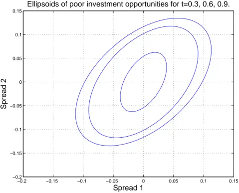
1-1 Ellipsoids. Ellipsoids of poor investment opportunities for N=2

con-vergence trades at times t = 0.3, 0.6, 0.9. . . 42

1-2 Weights for the case of uncorrelated spreads and collateral

constraint. Weights for the case of uncorrelated spreads. . . 45

1-3 VaR constraints, positive correlations. Wealth distribution at t = 0.25, 0.5, 0.75, 1 for an investor who invests in two positively correlated (ρ = 0.5) convergence trades, while facing VaR constraints (K=1).

Initial wealth is $100. . . 48

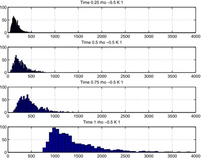
1-4 VaR constraints, negative correlations. Wealth distribution at t = 0.25, 0.5, 0.75, 1 for an investor who invests in two negatively cor-related (ρ = −0.5) convergence trades, while facing VaR constraints

(K=1). Initial wealth is $100. . . 48

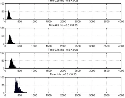
1-5 VaR constraints, positive correlations, tight constraints. Wealth distribution at t = 0.25, 0.5, 0.75, 1 for an investor who invests in two positively correlated (ρ = 0.5) convergence trades, while facing VaR

constraints (K=0.25). Initial wealth is $100. . . 49

1-6 VaR constraints, negative correlations, tight constraints. Wealth distribution at t = 0.25, 0.5, 0.75, 1 for an investor who invests in two negatively correlated (ρ = −0.5) convergence trades, while facing VaR

(10)

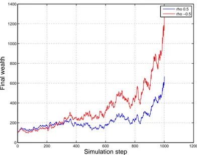
1-7 Wealth evolution under VaR constraint. Typical path of the wealth evolution for an investor investing in two convergence trades using the same noise process for positive and negative correlation under

the VaR constraint. Initial wealth is $100. . . 50

1-8 Relation between final wealth and frequency the VaR

con-straint binds. Final wealth is negatively correlated to the percentage

of time the constraints bind when the initial values of the convergence

trades are low. . . 50

1-9 Margin constraints, positive correlations. Wealth distribution at t = 0.25, 0.5, 0.75, 1 for an investor who invests in two positively cor-related (ρ = 0.5) convergence trades, while facing margin constraints

(Collateral = 1). Initial wealth is $100. . . 52

1-10 Margin constraints, negative correlations. Wealth distribution at t = 0.25, 0.5, 0.75, 1 for an investor who invests in two negatively cor-related (ρ = −0.5) convergence trades, while facing margin constraints

(Collateral = 1). Initial wealth is $100. . . 52

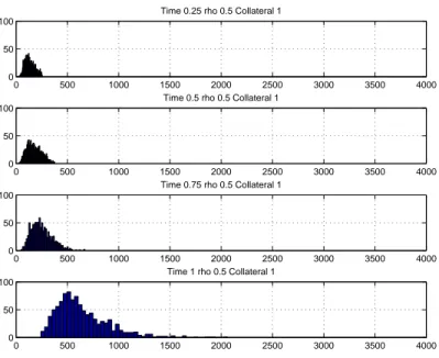
1-11 Margin constraints, positive correlations, more collateral needed. Wealth distribution at t = 0.25, 0.5, 0.75, 1 for an investor who invests in two positively correlated (ρ = 0.5) convergence trades, while facing

margin constraints (Collateral = 2). Initial wealth is $100. . . 53

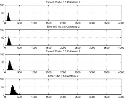
1-12 Margin constraints, negative correlations, more collateral needed. Wealth distribution at t = 0.25, 0.5, 0.75, 1 for an investor who invests in two negatively correlated (ρ = −0.5) convergence trades, while

fac-ing margin constraints (Collateral = 2). Initial wealth is $100. . . 53

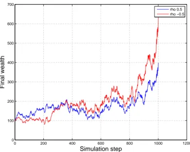
1-13 Wealth evolution under margin constraint. Typical path of the wealth evolution for an investor investing in two convergence trades using the same noise process for positive and negative correlation under

(11)

1-14 Relation between final wealth and frequency the margin

con-straint binds. Final wealth is negatively correlated to the percentage

of time the constraints bind when the initial values of the convergence

trades are low. . . 54

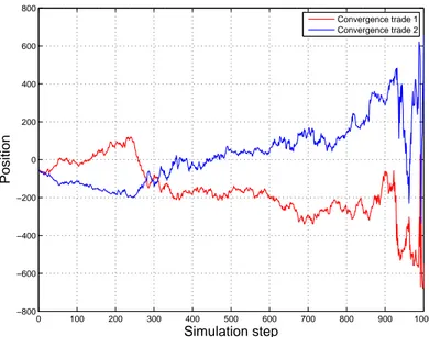
1-15 Positions evolution under VaR constraints. Typical path of the positions in two convergence trading opportunities under VaR

con-straints. . . 55

1-16 Positions evolution under margin constraints. Typical path of the positions in two convergence trading opportunities under margin

constraints. . . 55

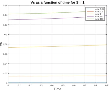
2-1 Partial derivative of the value function with respect to S for

a single convergence trade. VS as a function of time at S = 1

for different values of the robustness multiplier for a single convergence

trade. . . 76

2-2 Distortion drift for a single convergence trade. Distortion drift as a function of time at S = 1 for different values of the robustness

multiplier for a single convergence trade. . . 76

2-3 Distortion drift terms for a single convergence trade. Distor-tion drift terms as a funcDistor-tion of time at S = 1 for ν = 1 for a single convergence trade. The first term corresponds to a positive distor-tion drift that reduces the wealth of the investor since the investor is shorting the spread, while the second term corresponds to a negative

distortion drift that points to worse investment opportunities. . . 77

2-4 Optimal weight of a single convergence trade. Weight of the convergence trading strategy as a function of time at S = 1 for different

values of the robustness multiplier. . . 77

a single mean reversion trading strategy. VS as a function of

(12)

2-6 Distortion drift for a single mean reversion trading strategy. Distortion drift as a function of time at S = 1 for different values of

the robustness multiplier. . . 81

2-7 Distortion drift terms for a single mean reversion trading

strategy. Distortion drift terms as a function of time at S = 1

for ν = 1. The first term corresponds to a positive distortion drift that reduces the wealth of the investor, since the investor is shorting the spread, while the second term corresponds to a negative distortion

drift that points to worse investment opportunities. . . 81

2-8 Optimal weight of a single mean reversion trading strategy. Weight of the mean reversion trading strategy as a function of time at

S = 1 for different values of the robustness multiplier. . . 82

2-9 Optimal weights of two uncorrelated mean reversion trading

strategies for S1 = 1 and S2 = 2. Weights of the mean reversion

trading strategies as a function of time at S1 = 1 and S2 = 2 for

different values of the robustness multiplier. The correlation coefficient

is ρ = 0. . . 84

2-10 Ratio of the optimal weights. Ratio of the optimal weights of the

mean reversion trading strategies as a function of time at S1 = 1 and

S2 = 2 for different values of the robustness multiplier. The correlation

coefficient is ρ = 0. . . 84

2-11 Partial derivative of the value function with respect to S1 and

S2 at S1 = 1 and S2 = 2 when ρ = 0. Partial derivative of the value

function with respect to S1 and S2 as a function of time at S1 = 1 and

(13)

2-12 Optimal weights of two positively correlated mean reversion

trading strategies for S1 = 1 and S2 = 2. Weights of the mean

reversion trading strategies as a function of time at S1 = 1 and S2 =

2 for different values of the robustness multiplier. The correlation

coefficient is ρ = 0.5. . . 85

2-13 Optimal weights of two negatively correlated mean reversion

coefficient is ρ = −0.5. . . 86

strategies for S1 = 1 and S2 = 1. Weights of the mean reversion

is ρ = 0. . . 88

2-15 Ratio of the optimal weights at S1 = 1 and S2 = 1 when ρ = 0.

Ratio of the optimal weights of the mean reversion trading strategies

as a function of time at S1 = 1 and S2 = 1 for different values of the

robustness multiplier. The correlation coefficient is ρ = 0. . . 88

S2 at S1 = 1 and S2 = 1 when ρ = 0. Partial derivative of the value

function with respect to S1 and S2 as a function of time at S1 = 1 and

coefficient is ρ = 0. . . 89

(14)

S2 at S1 = 1 and S2 = 1 when ρ = 0.9. Partial derivative of

the value function with respect to S1 and S2 as a function of time at

S1 = 1 and S2 = 1 for different values of the robustness multiplier.

The correlation coefficient is ρ = 0.9. . . 90

2-19 Ratio of the optimal weights at S1 = 1 and S2 = 1 when ρ = 0.9.

Ratio of the magnitude of the optimal weights of the mean reversion

is ρ = 0.9. . . 90

coefficient is ρ = −0.8. . . 91

a single convergence trade when L = 0.1 and L = 100. VS

as a function of time at S = 1 for different values of the robustness multiplier. The solid line is when L = 100 and the dotted line is for

L = 0.1. . . 94

a single convergence trade when L = 0.1. VS as a function of

time at S = 1 for different values of the robustness multiplier. The

collateral constraint is |F | ≤ 0.1. . . 95

2-23 Optimal weight of a single convergence trade when L = 0.1. Weight of the convergence trading strategy as a function of time at S = 1 for different values of the robustness multiplier. The collateral

(15)

2-24 Optimal weight of a single convergence trade when L = 1. Weight of the convergence trading strategy as a function of time at S = 1 for different values of the robustness multiplier. The collateral

constraint is |F | ≤ 1. . . 96

2-25 Distortion drift for a single convergence trade when L = 0.1. Distortion drift as a function of time at S = 1 for different values of

the robustness multiplier. The collateral constraint is |F | ≤ 0.1. . . . 96

2-26 Distortion drift for a single convergence trade when L = 1. Distortion drift as a function of time at S = 1 for different values of

the robustness multiplier. The collateral constraint is |F | ≤ 1. . . 97

2-27 Distortion drift terms for a single convergence trade when L = 0.1. Distortion drift terms as a function of time at S = 1 for ν = 1 and L = 0.1. The first term corresponds to a positive distortion drift that reduces the wealth of the investor and it is bounded above due to the collateral constraint, while the second term corresponds to a

negative distortion drift that points to worse investment opportunities. 97

2-28 Distortion drift terms for a single convergence trade when L = 1. Distortion drift terms as a function of time at S = 1 for ν = 1 and L = 1. The first term corresponds to a positive distortion drift that reduces the wealth of the investor and it is bounded above due to the collateral constraint, while the second term corresponds to a

negative distortion drift that points to worse investment opportunities. 98

2-29 Optimal weight of a single convergence trade when L = 0.1 and L = 100. Weight of the convergence trading strategy as a function of time at S = 1 for different values of the robustness multiplier. The

(16)

2-30 Optimal weights of two uncorrelated convergence trades for

S1 = 1 and S2 = 2 when L = 0.5. Weights of the convergence trades

robustness multiplier. The correlation coefficient is ρ = 0 and the rhs of the VaR constraint is L = 0.5. . . 100

2-31 Value of the normalized wealth variance for two uncorrelated

convergence trades at S1 = 1 and S2 = 2 when L = 0.5. Value

of the normalized wealth variance for two uncorrelated convergence

trades as a function of time at S1 = 1 and S2 = 2 for different values

of the robustness multiplier. The correlation coefficient is ρ = 0 and the rhs of the VaR constraint is L = 0.5. . . 101

2-32 Optimal weights of two uncorrelated convergence trades for

robustness multiplier. The correlation coefficient is ρ = 0 and the rhs of the VaR constraint is L = 0.05. . . 101

of the robustness multiplier. The correlation coefficient is ρ = 0 and

the rhs of the VaR constraint is L = 0.05. . . 102

2-34 Optimal weights of two positively correlated convergence trades

for S1 = 1 and S2 = 2 when L = 0.05. Weights of the convergence

of the robustness multiplier. The correlation coefficient is ρ = 0.5 and

(17)

2-35 Value of the normalized wealth variance for two positively

cor-related convergence trades at S1 = 1 and S2 = 2 when L = 0.05.

Value of the normalized wealth variance for two positively correlated

convergence trades as a function of time at S1 = 1 and S2 = 2 for

dif-ferent values of the robustness multiplier. The correlation coefficient is ρ = 0.5 and the rhs of the VaR constraint is L = 0.05. . . 104 2-36 Optimal weights of two negatively correlated convergence trades

trades as a function of time at S1 = 1 and S2 = 2 for different values of

the robustness multiplier. The correlation coefficient is ρ = −0.5 and

2-37 Value of the normalized wealth variance for two negatively

correlated convergence trades at S1 = 1 and S2 = 2 when

L = 0.05. Value of the normalized wealth variance for two

nega-tively correlated convergence trades as a function of time at S1 = 1

and S2 = 2 for different values of the robustness multiplier. The

cor-relation coefficient is ρ = −0.5 and the rhs of the VaR constraint is L = 0.05. . . 105 2-38 Optimal weights of two uncorrelated convergence trades for

robustness multiplier. The correlation coefficient is ρ = 0 and the rhs of the VaR constraint is L = 0.05. . . 107 2-39 Value of the normalized wealth variance for two uncorrelated

of the robustness multiplier. The correlation coefficient is ρ = 0 and

(18)

2-40 Optimal weights of two positively correlated convergence trades

of the robustness multiplier. The correlation coefficient is ρ = 0.8 and

cor-related convergence trades at S1 = 1 and S2 = 1 when L = 0.05.

Value of the normalized wealth variance for two positively correlated

convergence trades as a function of time at S1 = 1 and S2 = 1 for

dif-ferent values of the robustness multiplier. The correlation coefficient is ρ = 0.8 and the rhs of the VaR constraint is L = 0.05. . . 109

2-42 Optimal weights of two negatively correlated convergence trades

for S1 = 1 and S2 = 1 when L = 8. Weights of the convergence

trades as a function of time at S1 = 1 and S2 = 1 for different values of

the robustness multiplier. The correlation coefficient is ρ = −0.8 and

correlated convergence trades at S1 = 1 and S2 = 1 when

L = 0.05. Value of the normalized wealth variance for two

nega-tively correlated convergence trades as a function of time at S1 = 1

and S2 = 1 for different values of the robustness multiplier. The

cor-relation coefficient is ρ = −0.8 and the rhs of the VaR constraint is L = 0.05. . . 110

2-44 Partial derivative of the value function with respect to S for a single mean reversion trading strategy and a collateral

con-straint with L = 0.7. VS as a function of time at S = 1 for different

(19)

2-45 Distortion drift terms for a single mean reversion trading

strategy and a collateral constraint with L = 0.7. Distortion

drift terms as a function of time at S = 1 for ν = 2 and for L = 0.7. The first term corresponds to a positive distortion drift that reduces the wealth of the investor, since the investor is shorting the spread, while the second term corresponds to a negative distortion drift that points to worse investment opportunities. The first term is bounded above due to the collateral constraint. . . 113

2-46 Optimal weight of a single mean reversion trading strategy

with a collateral constraint with L = 0.7. Weight of the mean

reversion trading strategy as a function of time at S = 1 for different values of the robustness multiplier and for L = 0.7. . . 114

2-47 Partial derivative of the value function with respect to S for a single mean reversion trading strategy with different

collat-eral constraints. VS as a function of time at S = 1 for different

values of the robustness multiplier and different collateral constraints. The solid line is for L = 70 and the dotted line for L = 0.7. . . 114

2-48 Optimal weight of a single mean reversion trading strategy

with different collateral constraints. Weight of the mean reversion

trading strategy as a function of time at S = 1 for different values of the robustness multiplier and different collateral constraints. The solid line is for L = 70 and the dotted line for L = 0.7. . . 115

strategies for S1 = 1 and S2 = 2 when L = 3. Weights of the

(20)

mean reversion trading strategies at S1 = 1 and S2 = 2 when

L = 3. Value of the normalized wealth variance for two uncorrelated

coefficient is ρ = 0 and the rhs of the VaR constraint is L = 3. . . 118 2-51 Optimal weights of two uncorrelated mean reversion trading

coefficient is ρ = 0 and the rhs of the VaR constraint is L = 2. . . 118 2-52 Value of the normalized wealth variance for two uncorrelated

coefficient is ρ = 0 and the rhs of the VaR constraint is L = 2. . . 119 2-53 Optimal weights of two uncorrelated mean reversion trading

coefficient is ρ = 0 and the rhs of the VaR constraint is L = 7. . . 119 2-54 Value of the normalized wealth variance for two uncorrelated

(21)

trading strategies for S1 = 1 and S2 = 2 when L = 7. Weights

of the mean reversion trading strategies as a function of time at S1 =

1 and S2 = 2 for different values of the robustness multiplier. The

correlation coefficient is ρ = 0.5 and the rhs of the VaR constraint is L = 7. . . 121

correlated mean reversion trading strategies at S1 = 1 and

S2 = 2 when L = 7. Value of the normalized wealth variance for two

positively correlated mean reversion trading strategies as a function

of time at S1 = 1 and S2 = 2 for different values of the robustness

multiplier. The correlation coefficient is ρ = 0.5 and the rhs of the VaR constraint is L = 7. . . 122

correlation coefficient is ρ = −0.5 and the rhs of the VaR constraint is L = 7. . . 122

negatively correlated mean reversion trading strategies as a function

multiplier. The correlation coefficient is ρ = −0.5 and the rhs of the VaR constraint is L = 7. . . 123

(22)

coefficient is ρ = 0 and the rhs of the VaR constraint is L = 2. . . 125

L = 2. Value of the normalized wealth variance for two negatively correlated mean reversion trading strategies as a function of time at

S1 = 1 and S2 = 1 for different values of the robustness multiplier.

The correlation coefficient is ρ = 0 and the rhs of the VaR constraint is L = 2. . . 125

correlation coefficient is ρ = 0.9 and the rhs of the VaR constraint is L = 2. . . 126

positively correlated mean reversion trading strategies as a function

multiplier. The correlation coefficient is ρ = 0.9 and the rhs of the VaR constraint is L = 2. . . 127

(23)

correlation coefficient is ρ = −0.5 and the rhs of the VaR constraint is L = 8. . . 127 2-64 Value of the normalized wealth variance for two negatively

negatively correlated mean reversion trading strategies as a function

multiplier. The correlation coefficient is ρ = −0.5 and the rhs of the VaR constraint is L = 8. . . 128

3-1 NIH time series flowchart. Flowchart for the construction of NIH appropriations time series. “NIH Approp.” denotes NIH appropria-tions; “PHS Gaps” denotes Institute funding by the U.S. Public Health Service; “Complete Approp.” denotes the union of these two series; “FY Change” allows for the change in government fiscal years; “4Q FY” time series refers to the resulting series in which all years are treated as having four quarters of three months each. . . 138 3-2 Appropriations data. NIH appropriations in real (2005) dollars,

categorized by disease group. . . 138

3-3 YLL time series flowchart. Flowchart for the construction of years of life lost (YLL) time series. “WONDER Chapter Age Group” refers to a query to the CDC WONDER database at the chapter level, strati-fied by age group at death; “US Pop.” is the United States population from census data as expressed in the WONDER dataset; and “US GDP” denotes U.S. gross domestic product. . . 140

(24)

3-4 YLL data. Panel (a): Raw YLL categorized by disease group. Panel (b): Population-normalized YLL (with base year of 2005), categorized

by disease group. Both panels are based on data from 1979 to 2007. 141

3-5 Efficient frontiers. Efficient frontiers for (a) all groups except HIV and AMS, γ = 0; (b) all groups except HIV and AMS, γ = 5; (c) all groups except HIV and AMS without the dementia effect, γ = 0; and (d) all groups except HIV and AMS without the dementia effect, γ = 5; based on historical ROI from 1980 to 2003. . . 148 4-1 Price of the risky asset as a function of the aggregate market

supply under varying constraints. We assume that we have 5

agents with the same risk aversion coefficients. The red plot assumes the same L = 30 for all the agents, while the blue assumes L to be

different across the agents L1 = 10, L2 = 20, L3 = 30, L4 = 40, L5 = 50. 163

4-2 Price of the risky asset as a function of the aggregate market

supply under tightening constraints. We assume that we have 5

agents with the same risk aversion coefficients. The blue plot assumes

L to be different across the agents L1 = 10, L2 = 20, L3 = 30, L4 =

40, L5 = 50 and the red assumes that each Li is reduced by 20%. . . . 164

supply with less variable constraints. We assume that we have 5

agents with the same risk aversion coefficients. The blue plot assumes

L to be different across the agents L1 = 10, L2 = 20, L3 = 30, L4 =

40, L5 = 50 and the red assumes that L1 = 20, L2 = 25, L3 = 30, L4 =

35, L5 = 40. . . 164

supply with constraints and varying risk aversions. We assume

that we have 5 agents with same constraints but different risk aversion coefficients. The blue plot assumes L = 30 for each agent, while the red line assumes that the agents are unconstrained. . . 166

(25)

4-5 Price of the risky asset as a function of the aggregate market supply with tightening constraints and varying risk aversions. We assume that we have 5 agents with same constraints but different risk aversion coefficients. The blue plot assumes L = 30 for each agent, while the red line assumes that L = 20 for each agent. . . 167

(26)

(27)

List of Tables

3.1 IoM recommendations. 12 major recommendations of the 1998

Institute of Medicine panel in four large areas for improving the process of allocating research funds. . . 133

3.2 ICD mapping. Classification of ICD-9 (1978–1998) and ICD-10 (1999–

2007) Chapters and NIH appropriations by Institute and Center to 7 disease groups: oncology (ONC); heart lung and blood (HLB); diges-tive, renal and endocrine (DDK); central nervous system and sensory (CNS) into which we placed dementia and unspecified psychoses to create comparable series as there was a clear, ongoing migration noted from NMH to CNS after the change to ICD-10 in 1999; psychiatric and substance abuse (NMH); infectious disease, subdivided into estimated HIV (HIV) and other (AID); maternal, fetal, congenital and pediatric

(CHD). The categories LAB and EXT are omitted from our analysis. 137

3.3 Return summary statistics. Summary statistics for the ROI of

disease groups, in units of years (for the lag length) and per-capita-GDP-denominated reductions in YLL between years t and t + 4 per dollar of research funding in year t−q, based on historical ROI from 1980 to 2003. . . 147

3.4 ROI example. An example of the ROI calculation for HLB from 1986. 147

3.5 Portfolio weights. Benchmark, single- and dual-objective optimal

portfolio weights (in percent), based on historical ROI from 1980 to 2003. . . 150

(28)

(29)

Chapter 1 Optimal trading of arbitrage

opportunities under constraints

In financial economics, an arbitrage is an investment opportunity that is too good to be true when there are no market frictions. In actual financial markets however, there are frictions and even if there are arbitrage opportunities the investors may not be able to fully exploit them due to the constraints they face.

We will explore two kinds of risky arbitrage opportunities when there are market frictions. The first one is a case of a textbook arbitrage, a convergence trade strategy. The second is a case of a statistical arbitrage, a mean reversion trading strategy. These two strategies are two of the most popular trading strategies that hedge funds follow, so studying them in detail when there are market frictions is a valuable exercise.

A convergence trade is a trading strategy consisting of long/short positions in two similar assets, where we buy the cheap asset, we short the expensive asset and we wait until the prices of the two assets to converge which we know it will happen for sure some particular time in the future. An example of this trade involves the difference in price between the the-run and the most recent off-the-run security. An on-the-run security is the most recently issued, and hence most liquid, of a periodically issued security. Since an on-the-run security is more liquid it trades at a premium to off-the-run securities [29]. A convergence trade involves taking a long position in the most recent off-the-run security and shorting the the-run security. The

(30)

on-the-run will become off-on-the-run upon the issue of a newer security and then there will be almost no difference between the two securities in our trade so their prices will converge. Another example involves investing in Treasury STRIPS with identical maturity dates but different prices.

A mean reversion trading strategy involves investing in an asset or a portfolio of assets whose value is a mean reverting process. Since most price series in the equity space follow random walk, this strategy most commonly involves investing in a port-folio of non-mean-reverting assets whose value is a stationary mean reverting series. These price series that can be combined in such a way are called cointegrating. A classic statistical arbitrage example is the pairs trading, which is the first type of algorithmic mean reversion trading strategy invented by institutional traders, report-edly by the trading desk of Nunzio Tartaglia at Morgan Stanley [64]. The statistical arbitrage pairs trading strategy bets on the convergence of the prices of two similar assets whose prices have diverged without a fundamental reason for this.

These arbitrage opportunities are risky under market frictions. In particular the first case is exposed to the “divergence risk”, i.e. the fact that the pricing differential between the two similar assets can diverge arbitrarily far from 0 prior to its conver-gence at some particular time in the future. The second case is exposed both to the “divergence risk” and to the “horizon risk”, in other words the fact that the times at which the spread will converge to its long run mean are uncertain.

We will explore the optimal portfolio allocation of a risk averse investor who invests in N convergence trades or mean reverting trading strategies, while facing constraints. In particular, we will study the optimal trading strategy when he faces VaR constraints or collateral constraints. Risk sensitive regulation, such as the VaR constraint, has lately become a central component of international financial regu-lations. Collateral or margin constraints, where the investor has to have sufficient wealth to secure the liabilities taken by short positions, have been ubiquitous in the financial transactions for centuries and margin calls have been behind several crises including the LTCM debacle[54].

(31)

will discuss about the setup of the model and the constraints, we will find the optimal trading strategy of the investor and finally we will explore the characteristics of this optimal strategy.

1.1 Literature review

Merton studied the problem of optimal portfolio allocation in a continuous time set-ting without any market frictions [59]. The optimal portfolio involves two terms: a market timing term and a hedging demand term. The first term is a myopic term that represents the optimal allocation if you were interested at each time instant t only for an horizon dt ahead. The second term represents the investor’s additional demand due to the covariance of the wealth process with the attractiveness of the available investment opportunities. Although Merton gives an analytical general solution this is expressed in terms of the partial derivatives of the value function and additional work is needed to derive the solution in terms of the model parameters. Additionally it assumes that there are no market frictions.

Optimal trading of mean reversion trading strategies have been studied by both Boguslavsky and Boguslavskaya [15] and Jurek and Yang [48]. They have found analytical solutions for the optimal weight of a single mean reverting trading strategy for risk averse CRRA investors. Their analysis is similar with the one in Kim and Omberg [49], where they assume that there is a risk free asset with a constant risk-free rate and a single risky asset with a mean reverting risk premium, which implies a mean reverting instantaneous Sharpe ratio. In all the cases they have assumed that there are no market frictions whatsoever.

Longstaff and Liu [53] have studied the problem of optimal trading of a single convergence trade under a margin constraint. For the single convergence trade case both VaR constraints and margin constraints collapse in the same constraint and the problem is significantly easier. In addition by studying only convergence trades they have taken out one important dimension of risk, the horizon risk, keeping only the divergence risk. Brennan and Schwarz [17] have also studied the problem of optimal

(32)

trading of a single convergence trade including transaction costs when the arbitrage potential is restricted by position limits.

The literature is rich with papers that study the existence of an equilibrium where there exists mispricings. This persistence of mispricings is typically attributed to agency problems, frictions or some kind of risk. Unlike textbook arbitrages, which generate riskless profits and require no capital commitments, exploiting real-world mispricings requires the assumption of some kind of risk. Shleifer and Vishny [74] emphasized that risks such as the uncertainty about when the pricing differential will converge to 0 and the possibility of a divergence of the mispricing prior to its elimination may play a role in limiting the size of positions that arbitrageurs are willing to take, contributing to the persistence of the arbitrage in equilibrium. Basak and Choitoru [6] also showed that arbitrage can persist in equilibrium when there are frictions. They study dynamic models with log utility and heterogeneous beliefs in the presence of margin requirements and other portfolio constraints.

With respect to the constraints, Basak and Shapiro [7] study the problem of opti-mal trading strategy of a risk averse investor who faces finite horizon VaR constraints in a complete markets setting using the martingale representation approach [4]. Here again there are no constraints in the optimal portfolio allocation at each time t but there is only one constraint in the wealth at some finite horizon. Finally, Geanakoplos [33] studies the collateral constraints, how these determine an equilibrium leverage and how this leverage changes over time, the so-called leverage cycles.

Let us now discuss about the setup of the model and the constraints and find the optimal trading strategy of the investor.

1.2 Analysis

We assume we have a risk averse investor maximizing the expected continuously compounded rate of return or equivalently the expected logarithm of his final wealth

E(lnWT). There are two cases to consider. In the first case, the investor can invest

(33)

Brownian bridges. In the second case, the investor can invest in a risk-free asset and N non-redundant mean reversion trading strategies, modeled as a multivariate Ornstein-Uhlenbeck (OU) process. The investor faces two kinds of constraints: VaR constraints or collateral constraints. We determine the optimal trading strategy and its characteristics in both cases.

1.2.1 Models

As we mentioned already, a convergence trade is a trading strategy consisting of long/short positions in two similar assets, where we buy the cheap asset, we short the expensive asset and we wait until the prices of the two assets to converge which we know it will happen for sure some time in the future. The spread of the convergence trade can be modeled as a Brownian bridge driven by K Brownian motions, which has the property that the spread will converge to 0 almost surely at some determined time in the future. The stochastic differential equation governing the spread of the trade is given by:

dSt= − aSt T − tdt + K X k=1 σkdZkt (1.1)

where St is the spread of the trade, a is a parameter controlling the rate of the mean

reversion to 0, T is the horizon of the investor which is also the time at which the

spread goes to 0 with probability 1 and Zt is a Brownian motion in RK. We can

see that the reversion to 0 grows stronger as t → T . Therefore, the investment opportunities get better as the spread gets larger and t → T , since then the drift term pushing the spread towards 0 gets larger.

A mean reversion trading strategy involves investing in a stationary portfolio of non-mean reverting assets, whose value is a mean reverting process. The value of the portfolio can be modeled as an Ornstein-Uhlenbeck (OU) process. The stochastic differential equation governing it is given by:

dSt= −φ(St− ¯S)dt +

K X

k=1

(34)

In our case we have N of these mean reverting processes and we assume that they are modeled as a multivariate Ornstein-Uhlenbeck process, which is defined by the following stochastic differential equation:

dSt= −Φ(St− ¯S)dt + σdZt (1.2)

Above Φ is a N-by-N square transition matrix that characterizes the deterministic

portion of the evolution of the process, ¯S is the vector representing the unconditional

mean of the process, σ is a N-by-K matrix that drives the dispersion of the process

and Zt is a Brownian motion in RK.

The Ornstein-Uhlenbeck process has the nice property that its conditional distri-bution is normal at all times, with mean equal to

Et[St+τ] = ¯S + e−Φτ(St− ¯S)

and covariance matrix independent of St[60]. We assume that Φ has eigenvalues with

positive real part, so that the conditional expectation approaches to ¯S as t → ∞.

The Ornstein-Uhlenbeck process captures the two important dimensions of risk in all relative value trades: the “horizon risk”, in other words the fact that the times at which the spread will converge to its long run mean are uncertain and the “divergence risk”, i.e. the fact that the pricing differential can diverge arbitrarily far from its long run mean prior to its convergence. The Brownian bridge captures only the “divergence” risk, since by its definition we assume that the investor has perfect information about the magnitude of the mispricing at some future date T , i.e. we assume that the date T on which the mispricing will be eliminated is known ahead with certainty.

1.2.2 Constraints

We consider two kinds of constraints: VaR and collateral constraints. The VaR constraint is a widely used statistical risk measure, adopted both by the regulators

(35)

and the private sector. It is the cornerstone of the capital regulations adopted by Basel regulations. Both the 1996 market risk amendment of the original 1988 Basel accord and the Basel II regulations have been built on the notion of Value-at-Risk [47]. The Value at risk (VaR) at α-level is defined as the threshold value such that the probability of losses greater than the threshold is less than α. In our case we consider instantaneous VaR constraints which amount for determining an upper bound in the wealth volatility, since locally the diffusion processes have normal distributions. Therefore, the instantaneous VaR constraints are given by:

θT_{Σθ ≤ LW}2

where θ is a N by 1 vector of positions, Σ is the instantaneous covariance matrix of the spreads, L is some proportionality constant that determines the tightness of the constraint and W is the investor’s wealth.

Collateral or margin constraints have been ubiquitous in the financial transactions for centuries. Even Shakespeare in the “Merchant of Venice” points out the importance of the collateral, as Shylock charged Antonio no interest rate but he asked for a pound of flesh as a collateral. The collateral constraints provide protection against mark-to-market losses whenever an investor generates a liability by shorting an asset. Therefore, they require that the investor’s wealth is bounded below by the collateral necessary to secure the liabilities. They are given by:

N X

i=1

λi|θi| ≤ W

where λi is the collateral necessary to secure the liability in spread i. In our work, each

unit of arbitrage should be understood as being relative to a fixed face or notional

amount and therefore each λi is a percentage of this fixed face value or notional

(36)

1.2.3 Solution

Let us now find the optimal trading strategy of a risk averse investor who maximizes

the expected logarithm of his final wealth E(lnWT). We consider two cases:

• The investor invests in the risk free asset and in N correlated convergence trades.

• The investor invests in the risk free asset and in N correlated mean reversion trading strategies.

For both cases our analysis is similar. For both cases we have:

Wt=

N X

i=1

θitSit+ θ0tB0t∀t ∈ [0, T ] (1.3)

where θit is the investor’s position in opportunity i for i = 1, · · · , N, θ0t is the

in-vestor’s position in the risk free asset, Sit is the spread of the convergence trade or

the value of the mean reverting portfolio and B0t is the price of the risk free asset.

The process θt is adapted to the filtration generated by the Brownian motion Zt.

The investor solves the following problem:

maximizeθ∈Θ E(lnWT)

subject to

dWt=PN_i=1θitdSit+ θ0tdB0t

dSt= µ(S, t)dt + σ(S, t)dZt

(1.4)

where Θ is the set of admissible trading strategies. Let us first define ∀t ∈ [0, T ] Ft=

(37)

For the convergence trades case, investor’s wealth satisfies the following stochastic differential equation: dWt= Wtrdt + N X i=1 θitSit(− ai T − t − r)dt + θ T_σdZ t dWt Wt = rdt + N X i=1 FitSit(− ai T − t − r)dt + F T_σdZ t

By applying Ito’s Lemma we have that:

d(ln(Wt)) = rdt + N X i=1 FitSit(− ai T − t− r)dt − 1/2F T t ΣFtdt + FtTσdZt Therefore it is: ln(WT) = ln(Wt) + Z T t rsds + Z T t N X i=1 FisSis(− ai T − t − rs) − 1 2F T s ΣFs ! ds + Z T t F_sTσdZs (1.5)

Assuming constant interest rate, we have:

Et(ln(WT)) = ln(Wt) + r(T − t) + Et Z T t N X i=1 FisSis(− ai T − t− rs) − 1 2F T s ΣFs ! ds ! + Et( Z T t F_sTσdZs) (1.6)

(38)

For the mean reversion trading strategies case, investor’s wealth satisfies the following stochastic differential equation:

dWt= Wtrdt + N X i=1 θit(−ΦTi (St− ¯S) − rSit)dt + θTσdZt dWt Wt = rdt + N X i=1 Fit(−ΦTi (St− ¯S) − rSit)dt + FtTσdZt

where Φi is the i’th row of the transition matrix Φ. By applying Ito’s Lemma we

have that: d(ln(Wt)) = rdt + N X i=1 Fit(−ΦTi (St− ¯S) − rSit)dt − 1/2FtTΣFtdt + FtTσdZt Therefore it is: ln(WT) = ln(Wt) + Z T t rsds + Z T t N X i=1 Fis(−ΦTi (Ss− ¯S) − rSis) − 1 2F T s ΣFs ! ds + Z T t F_sTσdZs (1.7)

Assuming constant interest rate we have:

Et(ln(WT)) = ln(Wt) + r(T − t) + Et Z T t N X i=1 Fis(−ΦTi (Ss− ¯S) − rSis) − 1 2F T s ΣFs ! ds ! + Et( Z T t F_sTσdZs) (1.8)

Under VaR constaints it is:

(39)

Under the margin constraints it is: N X i=1 λi|Fit| ≤ 1 ∀t F_tTΣFt = N X i=1 N X j=1 FitFjtσij ≤ N X i=1 N X j=1 λiλj|Fit||Fjt| σij λiλj < C < ∞ ∀t

Therefore, for both the cases and both the constraints the integrand of the stochastic

integral belongs in H2_{, which is a sufficient condition for the stochastic integral to be}

a martingale. Consequently, Et(

RT

t FsTσdZs) is equal to 0.

Maximizing Et(ln(WT)) is equivalent to maximizing the third term is equations

(1.6), (1.8) for both the cases respectively. Let’s now stydy in detail the solution for both cases for both the constraints.

VaR constraint

Maximizing Et(ln(WT)) under the VaR constraint is equivalent to solving ∀t the

following QCQP: minimize F_tTµt+ 1 2F T t ΣFt subject to FT t ΣFt≤ L (1.9) where µt=      S1t(_{T −t}a1 + r) ... SN t(_{T −t}aN + r)      (1.10)

for the convergence trades case and

µt=      ΦT 1(St− ¯S) + rS1t ... ΦT N(St− ¯S) + rSN t      (1.11)

(40)

We can easily solve the problem 1.9 by applying the KKT conditions or by

ge-ometry (see Appendix). F_topt, λopt_t are optimal iff they satisfy the following KKT

conditions ([10]):

• Primal feasibility: FtT optΣFtopt≤ L

• Dual feasibility: λoptt ≥ 0

• Complementary slackness: λopt_t (F_tT optΣF_topt− L) = 0

• Minimization of the Lagrangean: F_topt= argmin L(Ft, λoptt )

By solving the KKT conditions (see Appendix for details) we find that:

θtopt =        −Σ−1_µ tWt if µTtΣ−1µt≤ L −rΣ−1µtWt µT_tΣ−1_µt L if µT tΣ−1µt≥ L

This is equivalently written as:

θoptt = −

Σ−1_µ

tWt

1 + λoptt

where 1 + λoptt = max 1,

r

µT

tΣ−1µt L

!

Let’s now discuss more the properties of the solution. The investor has logarithmic preferences. Therefore, he is a myopic optimizer - there is no hedging demand [59]. At each time t he looks dt ahead and decides how to trade in an optimal way. There are two cases to consider:

• Case 1: At time t: µT

tΣ−1µt ≤ L In this case, the optimal solution is the

unconstrained myopic optimal solution, since it satisfies the VaR constraint.

For the convergence trades case, this is equivalent to the spread St being in the

(41)

The volume of the ellipsoid Etis shrinking as t → T , since vol(E) =QNi=1( a 1

T −t+

r)−1_{pdet(Σ)vol(B(0, 1)) where B(0, 1) is the unit sphere. Figure 1-1 shows this}

shrinking ellipsoid at three time instants.

For the mean reversion trading strategies case, this is equivalent to the spread or

value of the trade being inside the convex set C = {S | (S− ¯S)T_((Φ+rI)T_Σ−1_(Φ+

rI))(S − ¯S) + 2r ¯STΣ−1(Φ + rI))(S − ¯S) ≤ L − r2S¯TΣ−1S}, which in the case¯

of r = 0 is the ellipsoid C = {S | (S − ¯S)T_(ΦT_Σ−1_{Φ)(S − ¯}_{S) ≤ L. If ¯}_{S = 0 this}

convex set is also an ellipsoid.

These ellipsoids characterize poor opportunities where the constraints are not active. What constitutes poor investment opportunities changes over time for the case of convergence trades, while it remains invariant for the mean reversion trades case. For the case of convergence trades, the same spreads initially can be considered poor investment opportunities, where the investor does not bind the constraint, he is more conservative, but after some time they can be considered good opportunities and the investor becomes more aggressive and binds the constraint.

Informally, when the investment opportunities are poor, the spreads are more likely to widen which then would lead to mark-to-market losses and the investor would not have sufficient wealth to take advantage the better investment oppor-tunities and simultaneously satisfy the VaR constraints. Therefore, the investor is more conservative.

• Case 2: At time t: µT

tΣ−1µt> L Now the unconstrained myopic optimal

solu-tion does not satisfy the VaR constraint. This case is equivalent to the spread

Stbeing outside the shrinking ellipsoid Etfor the convergence trades case or the

set C for the mean reversion trades case. Now the investment opportunities are good. The investor wants to invest the unconstrained optimal trading strategy, but due to the VaR constraint invests in the proportion of this optimal trading strategy necessary to satisfy the VaR constraint.

(42)

−0.2 −0.15 −0.1 −0.05 0 0.05 0.1 0.15 −0.2 −0.15 −0.1 −0.05 0 0.05 0.1 0.15

Ellipsoids of poor investment opportunities for t=0.3, 0.6, 0.9.

Spread 1

Spread 2

Figure 1-1: Ellipsoids. Ellipsoids of poor investment opportunities for N=2 conver-gence trades at times t = 0.3, 0.6, 0.9.

Margin constraint

Maximizing Et(ln(WT)) under the margin constraint is equivalent to solving ∀t the

following convex program:

minimize F_tTµt+ 1 2F T t ΣFt subject to PN i=1λi|Fit| ≤ 1 (1.12) µt=      S1t(_{T −t}a1 + r) .. . SN t(_{T −t}aN + r)     

for the convergence trades case and

µt=      ΦT 1(St− ¯S) + rS1t ... ΦT_(S t− ¯S) + rSN t     

(43)

for the mean reversion trading strategies case.

Let’s apply the KKT conditions. Ftopt, νtopt are optimal iff they satisfy the KKT

conditions:

• Primal feasibility: PN

i=1λi|Fit| ≤ 1

• Dual feasibility: ν_topt ≥ 0

• Complementary slackness: ν_topt(PN

i=1λi|Fit| − 1) = 0

• Minimization of the Lagrangean Ftopt= argmin L(Ft, λoptt )

This program cannot be solved analytically in general. Again there are two cases to consider.

• Case 1: At time t: kΛΣ−1_µ

tk1 ≤ 1 where Λ = diag(λ1, · · · , λN) In this case, the

optimal solution is the unconstrained myopic optimal solution, since it satisfies the margin constraint.

For the convergence trades, this is equivalent to having at time t: kΛΣ−1_A

tSk1 ≤

1 where Λ = diag(λ1, · · · , λN) and At= diag(_{T −t}a1 + r, · · · ,_{T −t}aN + r). In this case

we have that St is inside a “diamond” in N dimensional space, which shrinks

as t → T .

For the mean reversion trades, this is equivalent to having at time t: kΛΣ−1_(Φ(S

t−

¯

S) + rSt)k1 ≤ 1 where Λ = diag(λ1, · · · , λN).

Informally again, when the investment opportunities are poor, the spreads are more likely to widen which then would lead to mark-to-market losses and the in-vestor would not have sufficient wealth to take advantage the better investment opportunities and have enough wealth for the collateral necessary to secure the liabilities.

(44)

• Case 2: At time t: kΛΣ−1µtk1 ≥ 1 where Λ = diag(λ1, · · · , λN). Now the investment opportunities are good, the unconstrained myopic optimal solution does not satisfy the collateral constraint and the constraint binds at the optimal solution.

Uncorrelated opportunities

There is a special case when the trading opportunities are uncorrelated, where we can solve analytically the KKT conditions (see Appendix for details). In that case the optimal positions are given by:

θ_itopt = sign(−µit)(| µit λi| − ν opt t )+ σ2 i λi Wt (1.13)

We observe the following:

• First of all for the convergence trades, in case the spread is positive we short the spread as we would expect and in case it is negative we are long the spread. For

the mean reversion trades, the sign is the opposite of the sign of ΦT

i(St− ¯S)+rSit.

• Second, if µtis high relative to the collateral then the magnitude of the position

is higher.

• Third, if the variability of the opportunity is high the magnitude of the corre-sponding position is low.

• Finally the more interesting property of the solution is that it has a cutoff value,

the dual variable, and if the absolute value of µt over the collateral is greater

than the dual variable the position is different from zero otherwise the position is 0. It is: νtopt = 0 if N X|λ_iµ_it| σ2 i ≤ 1

(45)

and ν_topt > 0 if N X i=1 |λiµit| σ2 i > 1

The dual variable is 0 when the investment opportunities are poor. It is easy to see that when the margin constraint binds we have:

˜

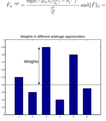
Fit opt =

sign(−µit)(|µit_λi| − νtopt)+

σ2 i λ2 i andk ˜F k1 = 1 (1.14) 1 2 3 4 5 6 0 0.1 0.2 0.3 0.4 0.5 0.6 0.7 0.8 0.9 1

Weights in different arbitrage opportunities.

Weights

Figure 1-2: Weights for the case of uncorrelated spreads and collateral

con-straint. Weights for the case of uncorrelated spreads.

In Figure 1-2 we can see an example of how we invest in different convergence trades when there is no correlation among them, with λ = 1 and volatilities equal

to 1 for all the opportunities. The height of each bar is the absolute value of µit

and we invest only in those spreads where the µit is larger than the dual variable.

If PN

i=1|µit| < 1, then the dual variable is 0, we invest in all the opportunities and

the collateral constraint does not bind. If PN

i=1|µit| > 1 as is in the figure then the

margin constraint binds, the dual variable is positive and we can find it as follows.

We start from the maximum µit and then reduce it until the sum of the weights is

(46)

1.2.4 Connection with Ridge and Lasso regression

Before we explore further the properties and the results of the optimal trading strate-gies, it would be interesting to digress for a while and see what connection there is between our problems and the regularized regressions.

In the basic form of regularized regression, the goal is not only to have a good fit, but also regression coefficients that are “small”. Two of the most common forms of regularized regressions are the Ridge and Lasso regression.

Ridge regression shrinks the regression coefficients by imposing a penalty on their size [42]. Equation 1.15 is one of the ways to write the Ridge problem.

minimize PN i=1(yi− β0− Pp j=1xijβj)2 subject to Pp j=1βj2 ≤ t (1.15)

The Ridge regression coefficients solution is similar to the optimal trading strategy followed by a risk averse investor with logarithmic preferences, who can choose among N diffusion processes and faces VaR constraints. In both cases we have this propor-tional shrinkage where we reduce all the weights by a constant.

Lasso regression is another common form of a regularized regression. It can be used as a heuristic for finding a sparse solution. It does a kind of continuous subset selection [16]. Equation 1.16 is one of the ways to write the Lasso problem.

minimize PN i=1(yi− β0− Pp j=1xijβj)2 subject to Pp j=1kβjk ≤ t (1.16)

The Lasso regression coefficients solution is similar to the optimal trading strategy followed by a risk averse investor with logarithmic preferences, who can choose among N diffusion processes and faces margin constraints. Therefore, we can expect that in this case we will have a sparse solution where the weights of several of the opportu-nities will be 0.

(47)

1.3 Results

Let us move on now to the results first for the convergence trades and then for the mean reversion trading strategies.

1.3.1 Convergence trades

VaR constraints. We have simulated the optimal trading strategy for N = 2

correlated convergence trading opportunities under VaR constraints. We find the following:

• It is often optimal for an investor to underinvest i.e. not to bind the constraint. • The investor typically experiences losses early before locking at a profit as we

can see in Figures 1-3, 1-4, 1-5, 1-6.

• Tighter constraints lead to less variability and less skewness in the distribution of wealth. They also lead to less final wealth as we can see in Figures 1-5, 1-6. • The wealth is higher when the opportunities hedge each other, as we can see in Figures 1-4, 1-6. This makes sense because when the constraints are binding we care more about losing money which would then lead surely to liquidation when the investment opportunities are better and therefore we prefer the op-portunities to hedge each other. Figure 1-7 shows a typical path for the wealth evolution using the same noise process for positive and negative correlation under the VaR constraint. We see clearly this hedging effect where negative correlation leads to more wealth.

• When the initial values of the convergence trades are low, the constraints bind for a small percentage of time and final wealth is negatively correlated to the percentage of time the constraints bind. Figure 1-8 shows this effect.

• The final portfolio wealth is highly positively skewed as it is obvious in Figures 1-3, 1-4, 1-5, 1-6

(48)

For all the simulations we used: σ1 = σ2 = 1, a1 = a2 = 1, S[0] = [1; 1], rf = 0.06, number of steps = 1000.

0 500 1000 1500 2000 2500 3000 3500 4000

0 50

100 Distribution of wealth Time 0.25 rho 0.5

0 500 1000 1500 2000 2500 3000 3500 4000

0 50

0 500 1000 1500 2000 2500 3000 3500 4000

0 50

0 500 1000 1500 2000 2500 3000 3500 4000

0 50

100 Distribution of wealth Time 1 rho 0.5

Figure 1-3: VaR constraints, positive correlations. Wealth distribution at t = 0.25, 0.5, 0.75, 1 for an investor who invests in two positively correlated (ρ = 0.5) convergence trades, while facing VaR constraints (K=1). Initial wealth is $100.

0 500 1000 1500 2000 2500 3000 3500 4000 0 50 100 Time 0.25 rho −0.5 K 1 0 500 1000 1500 2000 2500 3000 3500 4000 0 50 100 Time 0.5 rho −0.5 K 1 0 500 1000 1500 2000 2500 3000 3500 4000 0 50 100 Time 0.75 rho −0.5 K 1 0 500 1000 1500 2000 2500 3000 3500 4000 0 50 100 Time 1 rho −0.5 K 1

Figure 1-4: VaR constraints, negative correlations. Wealth distribution at t = 0.25, 0.5, 0.75, 1 for an investor who invests in two negatively correlated (ρ = −0.5) convergence trades, while facing VaR constraints (K=1). Initial wealth is $100.

(49)

0 500 1000 1500 2000 2500 3000 3500 4000 0 50 100 Time 0.25 rho 0.5 K 0.25 0 500 1000 1500 2000 2500 3000 3500 4000 0 50 100 Time 0.5 rho 0.5 K 0.25 0 500 1000 1500 2000 2500 3000 3500 4000 0 50 100 Time 0.75 rho 0.5 K 0.25 0 500 1000 1500 2000 2500 3000 3500 4000 0 50 100 Time 1 rho 0.5 K 0.25

Figure 1-5: VaR constraints, positive correlations, tight constraints. Wealth distribution at t = 0.25, 0.5, 0.75, 1 for an investor who invests in two positively cor-related (ρ = 0.5) convergence trades, while facing VaR constraints (K=0.25). Initial wealth is $100. 0 500 1000 1500 2000 2500 3000 3500 4000 0 50 100 Time 0.25 rho −0.5 K 0.25 0 500 1000 1500 2000 2500 3000 3500 4000 0 50 100 Time 0.5 rho −0.5 K 0.25 0 500 1000 1500 2000 2500 3000 3500 4000 0 50 100 Time 0.75 rho −0.5 K 0.25 0 500 1000 1500 2000 2500 3000 3500 4000 0 50 100 Time 1 rho −0.5 K 0.25

Figure 1-6: VaR constraints, negative correlations, tight constraints. Wealth distribution at t = 0.25, 0.5, 0.75, 1 for an investor who invests in two negatively correlated (ρ = −0.5) convergence trades, while facing VaR constraints (K=0.25). Initial wealth is $100.

(50)

0 200 400 600 800 1000 1200 0 200 400 600 800 1000 1200 1400 Simulation step Final wealth rho 0.5 rho −0.5

Figure 1-7: Wealth evolution under VaR constraint. Typical path of the wealth evolution for an investor investing in two convergence trades using the same noise process for positive and negative correlation under the VaR constraint. Initial wealth is $100. 0 0.1 0.2 0.3 0.4 0.5 0.6 0.7 0.8 0.9 1 0 200 400 600 800 1000 1200 1400 1600

Frequency the constraint binds

Final wealth

Figure 1-8: Relation between final wealth and frequency the VaR constraint

binds. Final wealth is negatively correlated to the percentage of time the constraints

(51)

Margin constraints. We have also simulated the optimal trading strategy for N = 2 correlated convergence trading opportunities under margin constraints using the same noise process as with the VaR constraints. We have similar results with the case of VaR constraints as we see in Figures 1-9, 1-10, 1-11, 1-12, 1-13 with the following important differences:

• When the constraints bind, it is often the case that the position in one of the convergence trades is 0, i.e. we have less diversification, sparse solution. Figure 1-15 shows a typical path of the positions in two convergence trading opportu-nities under VaR constraints, where we see that they tend to be different than 0. Figure 1-16 shows the evolutions of the positions in two convergence trading opportunities under margin constraints for the same exactly asset processes as before. We clearly see that often we invest only in one position, as we expected due to the similarity of the positions with the Lasso regression coefficients. • The final wealth is less skewed and smaller with respect to the case of VaR