HAL Id: hal-02635601
https://hal.inrae.fr/hal-02635601
Submitted on 27 May 2020
HAL is a multi-disciplinary open access
archive for the deposit and dissemination of
sci-entific research documents, whether they are
pub-lished or not. The documents may come from
teaching and research institutions in France or
abroad, or from public or private research centers.
L’archive ouverte pluridisciplinaire HAL, est
destinée au dépôt et à la diffusion de documents
scientifiques de niveau recherche, publiés ou non,
émanant des établissements d’enseignement et de
recherche français ou étrangers, des laboratoires
publics ou privés.
Using species distribution models to optimize vector
control in the framework of the tsetse eradication
campaign in Senegal
Ahmadou H. Dicko, Renaud Lancelot, Momar T. Seck, Laure Guerrini, Baba
Sall, Mbargou Lo, Marc J. B. Vreysen, Thierry Lefrancois, William M. Fonta,
Steven L. Peck, et al.
To cite this version:
Ahmadou H. Dicko, Renaud Lancelot, Momar T. Seck, Laure Guerrini, Baba Sall, et al.. Using species
distribution models to optimize vector control in the framework of the tsetse eradication campaign in
Senegal. Proceedings of the National Academy of Sciences of the United States of America , National
Academy of Sciences, 2014, 111 (28), pp.10149-10154. �10.1073/pnas.1407773111�. �hal-02635601�
Using species distribution models to optimize vector
control in the framework of the tsetse eradication
campaign in Senegal
Ahmadou H. Dickoa, Renaud Lancelotb,c, Momar T. Secka, Laure Guerrinid,e, Baba Sallf, Mbargou Lof, Marc J. B. Vreyseng, Thierry Lefrançoisb,c, William M. Fontah, Steven L. Pecki, and Jérémy Bouyera,b,c,1
aLaboratoire National d’Elevage et de Recherches Vétérinaires, Institut Sénégalais de Recherches Agricoles, BP 2057, Hann, Dakar, Sénégal;bUnité Mixte de
Recherche Contrôle des Maladies Animales Exotiques et Emergentes, Centre de Coopération Internationale en Recherche Agronomique pour le
Développement, 34398 Montpellier, France;cUnité Mixte de Recherche 1309 Contrôle des Maladies Animales Exotiques et Emergentes, Institut National de la
Recherche Agronomique, 34398 Montpellier, France;dUnité de Recherche Animal et Gestion Intégrée des Risques, Centre de Coopération Internationale en
Recherche Agronomique pour le Développement, 34398 Montpellier, France;eDepartment Environment and Societies, University of Zimbabwe, Harare,
Zimbabwe;fDirection des Services Vétérinaires, BP 45 677, Dakar, Sénégal;gInsect Pest Control Laboratory, Joint Food and Agriculture Organization of
the United Nations/International Atomic Energy Agency Programme of Nuclear Techniques in Food and Agriculture, A-1400 Vienna, Austria;hWest African
Science Center for Climate Change and Adapted Land Use, BP 13621, Ouagadougou, Burkina Faso; andiBiology Department, Brigham Young University,
Provo, UT 84602
Edited by Fred L. Gould, North Carolina State University, Raleigh, NC, and approved June 6, 2014 (received for review April 29, 2014)
Tsetse flies are vectors of human and animal trypanosomoses in sub-Saharan Africa and are the target of the Pan African Tsetse and Trypanosomiasis Eradication Campaign (PATTEC). Glossina palpalis gambiensis (Diptera: Glossinidae) is a riverine species that is still present as an isolated metapopulation in the Niayes area of Senegal. It is targeted by a national eradication campaign combin-ing a population reduction phase based on insecticide-treated tar-gets (ITTs) and cattle and an eradication phase based on the sterile insect technique. In this study, we used species distribution models to optimize control operations. We compared the probability of the presence of G. p. gambiensis and habitat suitability using a reg-ularized logistic regression and Maxent, respectively. Both models performed well, with an area under the curve of 0.89 and 0.92, respectively. Only the Maxent model predicted an expert-based classification of landscapes correctly. Maxent predictions were therefore used throughout the eradication campaign in the Niayes to make control operations more efficient in terms of deployment of ITTs, release density of sterile males, and location of monitoring traps used to assess program progress. We discuss how the mod-els’ results informed about the particular ecology of tsetse in the target area. Maxent predictions allowed optimizing efficiency and cost within our project, and might be useful for other tsetse con-trol campaigns in the framework of the PATTEC and, more gener-ally, other vector or insect pest control programs.
area-wide integrated pest management
|
genetic control|
aerial release|
chilled adult techniqueT
setse are vectors of human African trypanosomosis, a major neglected tropical disease (1), and African animal trypano-somosis (AAT), one of the most important pathological con-straints to livestock development in 38 infested African countries (2). The Pan African Tsetse and Trypanosomiasis Eradication Campaign is a political initiative started in 2001 that calls for intensified efforts to reduce the tsetse and trypanosomosis problem (3). As part of this global effort, the government of Senegal embarked in 2007 on a tsetse eradication campaign in a 1,000-km2 target area of the Niayes region, neighboring the capital Dakar. In this area, the limits of the distribution of the tsetse target populations were assessed using a stratified ento-mological sampling frame based on remote sensing indicators (4). The only tsetse species present was Glossina palpalis gam-biensis Vanderplank, and it was responsible for the cyclical transmission of three trypanosome species, namely Trypanosoma vivax, T. congolense, and T. brucei brucei, listed in order of im-portance (5). The high prevalence of animal trypanosomosis in the Niayes (serological prevalence of 28.7% for T. vivax) hamperedperi-urban intensification of cattle production (particularly dairy cattle). A population genetics study demonstrated that the G. p. gambiensis population of the Niayes was completely isolated from the main tsetse belt in the southeastern part of Senegal (6). This comprehensive set of entomological, veteri-nary, genetic, and other baseline data confirmed the isolated nature of the G. p. gambiensis population in the Niayes, which prompted the government of Senegal to select an eradication strategy using area-wide integrated pest management (AW-IPM) principles (7).
The successful implementation of an AW-IPM strategy re-quires a thorough understanding of the ecology of the target population, particularly its spatial distribution, a study which was undertaken in the Niayes from 2007 to 2011 before the start of the operational eradication efforts. The selected strategy inte-grates insecticide-treated targets (ITTs) and cattle with the re-lease of sterile insects. As the habitat of G. p. gambiensis is very fragmented (4), the targeting of suitable habitats for deployment of the ITTs is crucial to optimize cost efficiency (8) but also to enable the selection of appropriate sites for deployment of the
Significance
Tsetse flies transmit human and animal trypanosomoses in sub-Saharan Africa, respectively a major neglected disease and the most important constraint to cattle production in infested countries. They are the target of the Pan African Tsetse and Trypanosomiasis Eradication Campaign (PATTEC). Here we show how distribution models can be used to optimize a tsetse eradication campaign in Senegal. Our results allow a better understanding of the relationships between tsetse presence and various environmental parameters measured by remote sensing. Furthermore, we argue that the methodology de-veloped should be integrated into future tsetse control efforts that are planned under the umbrella of the PATTEC initiative. The results have a generic value for vector and pest control campaigns, especially when eradication is contemplated.
Author contributions: R.L., M.T.S., B.S., M.L., M.J.B.V., and J.B. designed research; A.H.D. and J.B. performed research; A.H.D., R.L., M.T.S., L.G., T.L., W.M.F., S.L.P., and J.B. contrib-uted new reagents/analytic tools; A.H.D., R.L., and J.B. analyzed data; and A.H.D., R.L., M.T.S., L.G., B.S., M.L., M.J.B.V., T.L., W.M.F., S.L.P., and J.B. wrote the paper.
The authors declare no conflict of interest. This article is a PNAS Direct Submission.
Freely available online through the PNAS open access option. 1To whom correspondence should be addressed. E-mail: bouyer@cirad.fr.
This article contains supporting information online atwww.pnas.org/lookup/suppl/doi:10. 1073/pnas.1407773111/-/DCSupplemental.
www.pnas.org/cgi/doi/10.1073/pnas.1407773111 PNAS | July 15, 2014 | vol. 111 | no. 28 | 10149–10154
APPLIE D BIOLOG ICAL SCIENC ES
monitoring traps to assess the impact of the control campaign. Although the initial entomological sampling was well-developed and efficiently implemented in the target area (4), we deem the development and use of population distribution models to be very beneficial in this regard.
The use of species distribution models to optimize vector or pest control is quite novel. The existing tsetse distribution models (SI Text) were critical for a better understanding of tsetse distri-bution and AAT epidemiology, but their spatial resolution was not sufficient to guide an eradication process. In this paper, we used high-resolution images and recent advances in species distribution modeling methods to improve prediction accuracy. Predictive models, and more specifically machine-learning methods, were used to model the distribution of G. p. gambiensis (9). Model choice has an impact on the final output and also depends on the available data. In this study, both presence and absence data were available, which is uncommon with respect to tsetse data. Therefore, following Brotons et al., we used both datasets (10). Understanding how predictions from presence–absence models relate to predictions from presence-only models is important, because presence data are more reliable than absence data.
Presence–absence data were modeled using a regularized logistic regression to avoid overfitting with respect to model parameters. There are various approaches to regularization for least square methods in statistical learning. The most widely used are the ridge regression and the lasso. Ridge regression bounds the regression coefficient space by adding the L2 norm (root square of the sum of squared values) of the coefficients to the residual sum of squares, whereas the lasso is a penalized least square method that shrinks the coefficient space by imposing an L1 penalty (sum of absolute values) on the regression coefficients. The elastic net framework used here is a compromise that com-bines ridge regression (L2 penalization) and the lasso (L1 penal-ization) for more flexibility in model selection (11). This model was chosen because of its flexibility and capacity to penalize complex models (12).
A Maxent model was in addition used to model presence-only data (13). This model, which is one of the most widely used to model species distributions, is a machine-learning method based on maximum entropy. Absence data are replaced with so-called background data, which are a random sample of the available en-vironment. Maxent fits a penalized maximum-likelihood model to avoid overfitting (L1 penalization). The logistic output from Maxent is a habitat suitability index rescaled to range from 0 to 1. Recently, the equivalence between Maxent and an infinitely weighted logistic regression was pointed out (14).
The relationship between occurrence and environmental data was explored with multidimensional exploratory analysis. For this purpose, we used the ecological factor niche analysis (ENFA) (15), which is a presence-only multidimensional method based on the concept of ecological niche (16).
The goal of this paper is to show how we selected among two competing approaches of species distribution modeling based on a large and accurate set of presence–absence data and how we used the results to optimize the eradication campaign in the Niayes of Senegal.
Results
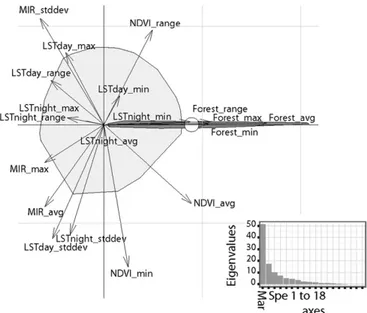
Ecological Niche.All of the variables associated with forest habi-tats and mean normalized difference vegetation index (NDVI) were highly correlated with the presence of G. p. gambiensis (Fig. 1). Conversely, night and day land surface temperature (LST) ranges and maximum middle infrared (MIR) were negatively correlated with the presence of G. p. gambiensis. High values of these variables corresponded to lower vegetation cover, reducing the buffering of macroclimatic conditions by the vegetation.
Standard deviations of MIR, NDVI, and day and night LST had high values on the specialization axis (SI Methods), whereas the environmental envelope for G. p. gambiensis was very narrow on this axis. This suggested that these satellite-derived parameters
captured important environmental features for the species for which variations were poorly tolerated.
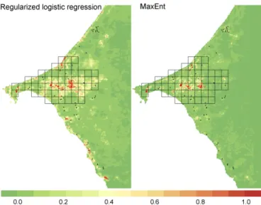
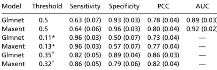
Model Outputs.Regularized logistic regression and Maxent pre-sented similar receiver operating characteristic (ROC) curves using the presence–absence validation dataset, with areas under the curve (AUCs) of 0.89 and 0.92, respectively (Fig. 2). Their predictions were highly correlated (Fig. S1; r= 0.68, P < 0.01; Fig. 3). Maxent presented a slightly better sensitivity using 0.5 as a threshold for presence, or the threshold allowing the best percentage of correctly classified (PCC) index, and a better specificity when the threshold was set to enable a sensitivity of 0.96 (Table 1). Using the expert-based landscape classification derived from aerial photography, Maxent predicted suitable habitats better than the regularized logistic regression (AUC 0.79 and 0.58; Fig. 2).
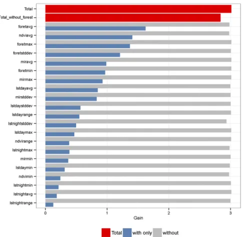
The regularized training gain (likelihood-based measure of model quality) of the Maxent habitat suitability model is pre-sented in Fig. S2. The Maxent models are presented using a single predictor or all of the predictors with the exception of the one of interest. The mean area of forest was the predictor giving the best gain when used alone, followed by the mean NDVI and the maximum forest area. These three predictors were highly correlated with each other along the ENFA marginality axis (Fig. 1 and SI Methods). Moreover, night LST SD had the highest negative effect on the gain (even if it was still very limited) when it was removed; thus, it contained specific information not accounted for by other predictors. The negative effect on the gain was the most prominent (6%) when all Landsat-related predictors (average, minimum, maximum, and SD of forest areas) were removed.
Fig. 1. First plan of the ecological niche factor analysis. The light gray polygon shows the overall environmental conditions available in the study area, the dark gray one shows environmental conditions where G. p. gam-biensis was observed (representation of the realized niche), and the small white circle corresponds to the barycenter of its distribution. The first axis (marginality axis) is a measure capturing the dimension in the ecological space in which the average conditions where the species lives differ from the global conditions; a large marginality value implies that the conditions where the species is found are“far” from the global environmental con-ditions. In contrast, the second axis (specialization) measures the narrowness of the niche (ratio of the multidimensional variances of the available to occupied spaces). The eigenvalues of the axes present the percentages of the global inertia explained by theses axes (69% for the first plan). avg, average; mar, marginality; max, maximum; min, minimum; forest, surface of forest landscapes (Landsat data); spe, specialization; stddev, SD.
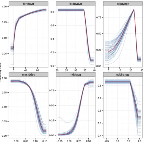
Marginal response curves for the different predictors (Fig. S3) showed that the percentage of the area covered by forest was positively correlated with habitat suitability, with a sharp increase after 5% of forests and a plateau after 20%. With respect to average day LST, habitat suitability was stable between 20 and 35 °C and then sharply decreased; whereas average day LST was not low enough in the study area to limit the presence of G. p. gambiensis, high temperatures were unsuitable. The cor-relation between minimum day LST and habitat suitability was bell-shaped, with a maximum between 20 and 25 °C. This could be related to the buffering effect of dense tree cover on tem-perature drops at night. Indeed, night temtem-perature drops faster in open environments than in the forest. Habitat suitability dropped sharply, with minimum temperatures exceeding 25 °C. The correlation between mean NDVI and habitat suitability was a sigmoid curve that increased sharply after 0.2. Regarding NDVI range, a plateau of habitat suitability was observed until 0.5 and sharply decreased after this threshold, thus illustrating the importance of perennial tree vegetation for this tsetse spe-cies. The relationship with habitat suitability was similar for MIR SD, related to the strong negative correlation between NDVI and MIR.
Use of Maxent Predictions in the Tsetse Eradication Project.Before the availability of the Maxent model in the Senegal project, operational choices such as selection of trap sites were made using a vegetation classification obtained from a Landsat 7 En-hanced Thematic Mapper Plus (ETM+) image of April 2001. Suitable habitat for G. p. gambiensis was mapped from this classification with high sensitivity but low specificity (4). The availability of the Maxent predictions was used in four ways to optimize the implementation of the eradication effort.
First, boundaries of the target eradication area, shown as black grid cells in Fig. 3, were validated by the model. All of the new suitable habitat areas identified by the Maxent model within a range of 5 km around sites where wild G. p. gambiensis had been trapped (at any occasion) were already included in the control strategy (Discussion). The target area was subdivided into four operational blocks, which are being sequentially addressed during the operational program (Fig. 4). Each block was sub-jected to a 1-y tsetse-density reduction phase, followed by an 18-mo eradication period using the sterile insect technique.
Second, the spatial distribution of the monitoring traps deployed since January 2012 in block 1 and since October 2012 in block 2 was modified through relocating 22 of the 97 moni-toring traps (23%) to more suitable sites according to habitat suitability as predicted by the Maxent model (Fig. S4). In block 3, where monitoring had not started yet at the time of writing, the monitoring traps will also be deployed in sites that have a high (predicted) suitability value as indicated by the model.
Third, 1,347 insecticide-impregnated traps used for tsetse-density reduction were deployed in block 2 according to predictions of
Maxent during the period December 2012 to February 2013, from which 661 were renewed during the period January to February 2014. The total surface area covered by block 2 is close to 500 km2 but contains only 80.6 km2of predicted suitable habitat, thus giving a final trap density of 16.7 traps per km2of suitable habitat (Fig. 4).
Fourth, predicted suitable habitats were also used to optimize aerial releases of sterile male G. p. gambiensis. Polygons with similar surface areas of suitable patches were identified (RL1 and RL2 in block 1, for example; Fig. 4) and the density of re-leased sterile males was adjusted proportionally to the area of suitable habitat in these polygons (0.24 and 0.11 flies per ha in RL1 and RL2, respectively).
Optimization of Tsetse Suppression and Eradication by the Model.In the first block, the apparent density of G. p. gambiensis dropped from an average of 0.42 (SD 0.39) flies per trap per d before control to an average of 0.04 (SD 0.11) flies per trap per d and 0.003 (SD 0.01) flies per trap per d during the suppression and eradication phases, respectively (Fig. 5). In the second block, the apparent density dropped from an average of 1.24 (SD 1.23) flies per trap per d before control to an average of 0.005 (SD 0.017) flies per trap per d during the suppression phase.
Apparent fly density in block 2 was higher than in block 1 (generalized linear mixed model, P= 0.009;SI Methods) before the start of the suppression, which initially sharply reduced tsetse densities (P= 0.001). This effect was limited in time (6 mo), and tsetse density remained stable and even increased with time thereafter (P < 10−3), although remaining at a very low level (<0.04 fly per trap per d) until the eradication phase started. The cumulated reduction of densities with time was higher in block 2 (reduction of 99.6%) than in block 1 (reduction of 90.4%) (P< 10−3).
In block 1, the last wild fly was captured on August 9, 2012, ∼6 mo after the start of sterile male releases. It was an old fe-male (more than 40 d old) in its fourth larviposition cycle with an empty uterus, and the next follicle was immature and small, in-dicating an abortion. This female showed a copulation scar and its spermatheca was 85% filled, indicating that its sterility was probably induced by a mate with one sterile male. From the beginning of the eradication phase in block 1 (March 16, 2012) to the date corresponding to the last capture, only three other wild
Fig. 2. ROC curves and AUCs of the regularized logistic regression and Maxent models. These results were obtained using the presence–absence validation dataset (Left) and the expert-based landscape classification from aerial images (Right).
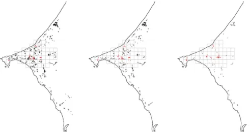
Fig. 3. Predictions of the regularized logistic regression and Maxent models. In the case of the logistic model, the predictions correspond to probabilities of presence, whereas in the case of the Maxent model, they correspond to a rescaled suitability index (logistic output). The black cells correspond to the target area. Black and red crosses represent absence and presence data, respectively.
Dicko et al. PNAS | July 15, 2014 | vol. 111 | no. 28 | 10151
APPLIE D BIOLOG ICAL SCIENC ES
females could be dissected and all had indications of having mated with a sterile male. The average percentage of sterile males as a proportion of all catches was then 99.2% (SD 1.6%), corresponding to a sterile-to-wild male ratio of 130. The percentage of sterile males remained 100% thereafter (no wild fly was captured for 78 weekly collections with 25 monitoring traps), corresponding to a very likely eradication (probability of not detecting potential remaining flies of 0.002 only).
Discussion
Ecological Niche of G. p. gambiensis in the Niayes. Our analysis showed that the ecological niche of G. p. gambiensis in the Niayes area corresponded to permanent ligneous vegetation with a tree density sufficient to provide adequate shade and buffer tem-perature and relative hygrometry variations in comparison with macroclimatic conditions occurring in the surrounding open environments. Air temperature in dense tree vegetation in gal-lery forests can be 4 °C lower compared with the surroundings, and relative humidity 15% higher. This habitat provides resting sites for G. p. gambiensis in contrast to the more open habitat into which they may disperse for short periods (some hours) in search of a blood meal, namely their hunting sites. Suitable G. p. gambiensis habitat may be seasonal because of the variations of macroclimatic conditions and of nonpermanent vegetation.
The Maxent model confirmed that permanent dense tree vegetation was important for G. p. gambiensis, but also that the larger the area occupied by the flies during the rainy season (corresponding to their dispersal capacity) the more suitable this habitat appears to be for G. p. gambiensis. Evidence is provided by the positive correlation of the forest range with the ENFA marginality axis (Fig. 1).
The data layers derived from Landsat images, which have a higher spatial resolution (30 m) than Moderate Resolution
Imaging Spectroradiometer from the National Aeronautics and Space Administration (MODIS) data (250 m), were important predictors of the presence of G. p. gambiensis. This was expected, given their ability to survive in very small vegetation patches in the Niayes (4). It would be difficult to obtain such fine-scale data for larger regions of West Africa. Fortunately, a good correlation was found between forest predictors and minimum night LST (Fig. 1). Moreover, the regularized gain is only reduced by 6% when all forest predictors are removed.
Comparison of the Regularized Logistic Regression and Maxent Models.
The nature of predictions differs between regularized logistic re-gression (probability) and Maxent (index). However, the two pre-dictions were highly correlated, as observed elsewhere (17). Model quality-assessment metrics were similar using the presence–absence validation dataset. Maxent predicted suitable areas better than regularized logistic regression based on the expert-based land-scape classification. Tsetse presence data are generally more meaningful than absence data, because all known traps have a very low efficiency with respect to trapping rates (as a percentage of available individuals), namely≤1% per d per km2(4). In the Niayes, observed trapping efficiencies were as low as 0.3% per d per km2following the release of more than 200,000 sterile male flies. In our case, particular conditions (feasibility study of an eradication project) allowed a rigorous selection of false absen-ces (SI Methods), including homogeneous trapping protocol and known trap efficiency (4). Under other circumstances (trap ef-ficiency unknown, different trap models, or trapping protocols), trapping may generate false absence data. Using only presence data to assess habitat suitability has the advantage that data de-rived from different sources (e.g., compilation of published data) can be combined to inform control projects.
Moreover, Maxent predictions were important for the eradi-cation program as all suitable habitat needed to be included in the monitoring and the target area, even if they were not infested at the time of sampling due to possible movement among the patches. In the Niayes area, G. p. gambiensis are never present in all suitable patches at the same time. Instead, they form a metapopulation with patches connected through dispersal (18).
Use of Model Predictions for Optimization of the Eradication Project.
To generate a binary presence–absence map to delimitate the infested area, we chose a threshold providing a high sensitivity (96%). Indeed, in the case of an eradication project, it is para-mount to reduce false negatives as much as possible, to avoid leaving tsetse-infested pockets not subjected to the control ef-fort. Such areas can act as a source of reinvasion into previously cleared areas. During the entomological baseline data survey, the target area was divided into operational 5× 5 km grid cells where at least one tsetse had been captured, plus a buffer zone
Table 1. Prediction qualities of the regularized logistic regression and Maxent models using the validation dataset Model Threshold Sensitivity Specificity PCC AUC Glmnet 0.5 0.63 (0.07) 0.93 (0.03) 0.78 (0.04) 0.89 (0.03) Maxent 0.5 0.64 (0.06) 0.96 (0.03) 0.80 (0.04) 0.92 (0.02) Glmnet 0.11* 0.96 (0.03) 0.50 (0.07) 0.73 (0.04) — Maxent 0.13* 0.96 (0.03) 0.57 (0.07) 0.77 (0.04) — Glmnet 0.35† 0.82 (0.05) 0.89 (0.04) 0.86 (0.03) — Maxent 0.32† 0.86 (0.05) 0.79 (0.06) 0.82 (0.04) —
These results were obtained with the presence–absence validation dataset. SDs are presented in parentheses. Glmnet, regularized logistic regression. *Selected to optimize sensitivity.
†Selected to optimize PCC.
Fig. 4. Optimization of the integrated control strat-egy using model predictions. The Maxent model was used with a threshold of 0.13 to predict the suitable habitats for G. p. gambiensis (sensitivity of 0.96 and specificity of 0.57). In block 1, the suitable habitats allowed delimitating two polygons for aerial releases (RL1 and RL2) where the minimum numbers of sterile males released per km2were 24 and 11, respectively,
based on Maxent predictions. Adult chilled tsetse flies are released with a Mubarqui smart release machine on board a gyrocopter of the Kalahari aerodrome (Upper Left) (20). In block 1, the green and gray lines represent the track flying records of the gyrocopter on April 14, 2014 in RL1 and April 11, 2014 in RL2, respectively. In block 2, 1,347 insecticide-impregnated traps were set from December 2012 to February 2013 in the predicted suitable sites (blue lozenges) to sup-press tsetse populations.
consisting of the grid cells contiguous to these infested cells. This strategy was validated by the Maxent predictions using this sensi-tivity threshold and confirmed that the target area was spatially isolated from any other suitable area for G. p. gambiensis. The area selected for model predictions did not include the populations of northern Sine Saloum (4) because they represent a different eco-type, genetically isolated from the Niayes metapopulation. We however included the“small coast” area of Senegal, again to avoid leaving tsetse-infested pockets south of the target area (6).
Interestingly, the Maxent model predicted some suitable habitat north of the target area (Fig. 3), which was infested by G. p. gambiensis in the 1970s and was subjected to a control pro-gram using residual spraying of dieldrin and trapping (4). This former control program probably eliminated some pockets of G. p. gambiensis that were completely isolated from the main infested area by sand dunes. Actually, no G. p. gambiensis flies were captured in these sites despite intensive sampling for several months and using numerous traps (4), despite these sites appearing fully suitable for this species based on phytosociological criteria.
The improvement provided by the Maxent model, in com-parison with the maps of suitable habitats (forests) based on the supervised classification of Landsat ETM+ images, is mainly related to specificity: 0.43 with this classification vs. 0.57 with Maxent. Sensitivity was already 0.96 with the supervised classi-fication. Maxent selected those permanent tree habitats where climatic conditions (particularly temperature) allowed tsetse sur-vival. Even if MODIS data mainly provide information on the macroclimate, they also allow making inferences on tree cover (particularly using night LST) and therefore on the buffering ef-fect of permanent vegetation on macroclimatic conditions. Maxent models thus allowed increasing the sensitivity of the monitoring system, because traps previously set in unsuitable habitats have been moved based on suitability predictions (Fig. S4).
Regarding the suppression strategy, the use of the vegetation classification in block 1 (Maxent predictions were not available then) already represented a great improvement in comparison with previous tsetse control programs; 269 targets were set in block 1 from December 2010 to February 2011 using this clas-sification (corresponding to 19.4 targets per km2 of suitable habitat). They allowed a good suppression of the flies, whereas in the absence of a model of suitable habitat, densities of 60 targets per km2were required in Guinea against the same subspecies: Recently, on Fotoba Island, 30 targets per km2could only reduce the apparent fly density by 62% (8). In block 2, Maxent further improved the results, and a significantly higher reduction rate (99.6%) than in block 1 was obtained with a lower target density of 16.7 targets per km2of suitable habitat (and 2.7 targets per km2 of the target area only). Considering a target cost of V3 in our project and a deployment cost ofV6 per trap (19), the total re-duction of the costs can be estimated at∼V43,700 for 1,000 km2. Moreover, Maxent predictions allowed concentrating the re-lease of sterile flies onto suitable habitats in block 1: With only 16.5 (SD 7.0) sterile flies released weekly per km2, a sterile-to-wild male ratio of 130 was obtained, inducing 100% sterility in females and thus driving the population to extinction. The minimal weekly release rate was set at 10 and 100 flies per km2of unsuitable and suitable habitat, respectively. Initially, sterile males were released from the air using carton boxes dropped from a gyrocopter, but since February 2014 a more advanced automatic chilled adult release machine was used (Mubarqui smart release machine; Fig. 4) that can be parameterized daily considering these parameters and the amount of flies available at the emergence center (Senegalese Institute for Agricultural Research) (20, 21). Within this machine, the vibratory feeders can be adjusted to release rates between 10 and 100 flies per km2, with a gyrocopter flying at a speed of 110 km/h. In the ab-sence of the Maxent models, it would have been necessary to release at least 100 flies per km2everywhere in the target area [in Zanzibar, up to 300 flies per km2were even released in the forest section to eradicate G. austeni (22)]. With a mean cost ofV0.2 per pupa [including production costs at Centre International de Recherche-Développement sur l’Elevage en zone Subhumide (CIRDES), Burkina Faso and the Slovak Academy of Sciences (SAS) andV0.04 transport cost per pupa], this represents major savings of ∼V590,000 for our project, taking into account that 70% of received pupae provide for operational sterile flies, when taking into account the emergence rate and mortality rate at the insectarium before release. Moreover, the total number of sterile male G. p. gambiensis pupae produced by the CIRDES and the SAS is currently limited to 25,000 pupae per wk, and treating the full area would not have been possible without adjusting release densities to the availability of suitable habitat.
The same methodology will be applied in the two remaining blocks following the rolling carpet approach: When eradication is started in a given block, suppression is started in the contig-uous block to avoid any risk of reinvasion. Based on this strategy, the full target area is planned to be cleared from tsetse by the end of 2016.
The same approach might be used to optimize any vector or insect pest control program, especially when eradication is the selected strategy (23).
Methods
Site Description. The study area had a total surface of 7,150 km2, located in
the Niayes region of Senegal (14.1° to 15.3° N and 16.6° to 17.5° W). At the time of the study, it was the target of an eradication campaign against an isolated G. p. gambiensis population (4) (Fig. 4). The climate is hot and dry from April to June, whereas the rainy season occurs from July to October and the cold dry season from November to March.
Response Data. Learning dataset. A cross-sectional survey was implemented from December 2007 to March 2008 (dry season) to collect baseline data for the eradication campaign using 683 unbaited Vavoua traps (4). Traps were Fig. 5. Impact of the control operations on tsetse apparent densities per
trap per d. The red vertical lines represent the start of the suppression phase (insecticide targets) in each block, whereas the blue vertical lines represent the start of the eradication phase (release of sterile males). Densities are presented in natural log scale [log (catch+ 1)]. The regression curves cor-respond to a nonparametric loess curve with associated 95% confidence interval. The map presents the location of the blocks that are targeted se-quentially following a rolling carpet approach. The vertical red arrow shows the capture of the last indigenous fly in block 1.
Dicko et al. PNAS | July 15, 2014 | vol. 111 | no. 28 | 10153
APPLIE D BIOLOG ICAL SCIENC ES
removed as soon as a tsetse fly was caught (minimum 1 d). In the absence of capture, the traps were retrieved after a maximum of 42 d.
To homogenize data quality and avoid pseudoreplication (data points in the same pixel), the dataset was simplified in two ways. First, the study area was rasterized into square pixels with a 250-m resolution to match the model predictors (SI Methods).
For the presence data, all trap positions located within the same pixel were aggregated and concentrated in the pixel center. Presence data were ob-served in 68 pixels from 91 presence points (Fig. S5).
For the absence data, all trap positions located within a buffer of 500 m around a presence point were removed (to account for tsetse dispersal capacity). Furthermore, we removed absence pixels with P> 0.01 that the flies were present despite the absence of trapping using the model described (24) (SI Methods). From the initial 592 absence data, 333 were finally retained (Fig. S5), 56 of which were used in the validation dataset. Therefore, the training dataset was composed of 68 presence and 269 absence data. Validation datasets. Trap data were collected independent of the training dataset from April 2009 to February 2013 during different surveys (tsetse dispersal and competitiveness studies, longitudinal monitoring of the de-mographic structure of tsetse populations, etc.). This dataset included 92 presence and 64 absence data. It was processed as described above, resulting in a dataset of 64 presence and 1 absence data (trapping times were not long enough to ascertain tsetse absence). A subset of 56 absence data was ex-tracted from the 333 absence data described above.
A second validation dataset was created using 182 aerial photos taken from a gyrocopter at an altitude ranging from 100 to 300 m. The environment identified from these pictures was subsequently categorized as suitable or unsuitable for tsetse habitat (4). Picture coordinates were corrected using Google Earth to take the angle and deviation from the ground into account. Overall, 23 suitable and 159 unsuitable habitats were identified, thereafter called“expert-based habitats” (Fig. S6).
Predictors Used for Tsetse Suitable Habitat. Climatic and environmental data were derived from a time series of MODIS (version V005). Composite day and night land surface temperature (MOD11A2; 8-d averages), middle infrared (MOD13Q1; 16-d averages), and normalized difference vegetation index (MOD13Q1; 16-d averages) were selected for the analysis (25). Spatial resolution of pixels was 250× 250 m (SI Methods).
A supervised classification of the vegetation was achieved using Landsat 5 Thematic Mapper satellite images with a spatial resolution of 30× 30 m (SI Methods). Four cloud-free and haze-free satellite images were used, from
October 2009, April 2010, June 2010, and December 2010, to take into ac-count the seasonal dynamics of these habitats, named“forests” in the manuscript.
Models. Ecological niche factor analysis was used to characterize the habitat of G. p. gambiensis in the target area (SI Methods).
Regularized logistic model was used to predict tsetse presence probability. Maxent analysis was used to predict habitat suitability. Approximately 10,000 pixels were sampled from the environmental variables (background) to calibrate the model. Because of the small sample size for presence data (56 points), only linear and quadratic transformations of environmental variables were used. Model performance and comparison were assessed using the two vali-dation sets (26). Model performance metrics were computed for each pre-dictive model (27). The metrics used were the area under the receiver operating curve, called the area under the curve (28), the percentage of consonants correct (PCC), the specificity, and the sensibility (SI Methods). Regularized gain is an additional metric for Maxent models. Marginal response curves were also computed to assess the relationship between the predicted suitability index and a given environmental datum. These curves were obtained by varying this variable while keeping all others at their average value.
Predicted values from regularized logistic regression and Maxent models were compared using Spearman’s rank correlation coefficient.
Impact of Control Operations. We used a generalized linear mixed model (29) to measure the impact of the suppression on tsetse apparent densities. The response data were tsetse counts in the traps. Time (measured in weeks), treatment (suppression or not), and the block (1 or 2) and their interactions were used as fixed effects, whereas the trap locations were used as random effects (SI Methods). Raw data are presented inDataset S1.
The probability that eradication was effective in block 1 was estimated using the same model used to clean the absence dataset (24) (SI Methods), considering that at least a couple of flies were necessary to maintain the population.
ACKNOWLEDGMENTS. This work was funded by the US State Department through the Peaceful Uses Initiative, the Joint Food and Agriculture Orga-nization of the United Nations/International Atomic Energy Agency Division of Nuclear Techniques in Food and Agriculture, the Department of Technical Cooperation, the Directorate of Veterinary Services of Sénégal, Institut Sénégal-ais de Recherches Agricoles, and Centre de Coopération Internationale en Recherche Agronomique pour le Développement.
1. Simarro PP, Jannin J, Cattand P (2008) Eliminating human African trypanosomiasis: Where do we stand and what comes next? PLoS Med 5(2):e55.
2. Itard J, Cuisance D, Tacher G (2003) Trypanosomoses: Historique - répartition géo-graphique. Principales Maladies Infectieuses et Parasitaires du Bétail. Europe et Ré-gions Chaudes, eds Lefèvre P-C, Blancou J, Chermette R (Lavoisier, Paris), Vol 2, pp 1607–1615.
3. Kabayo JP (2002) Aiming to eliminate tsetse from Africa. Trends Parasitol 18(11): 473–475.
4. Bouyer J, et al. (2010) Stratified entomological sampling in preparation for an area-wide integrated pest management program: The example of Glossina palpalis gam-biensis (Diptera: Glossinidae) in the Niayes of Senegal. J Med Entomol 47(4):543–552. 5. Seck MT, Bouyer J, Sall B, Bengaly Z, Vreysen MJB (2010) The prevalence of African animal trypanosomoses and tsetse presence in western Senegal. Parasite 17(3): 257–265.
6. Solano P, et al. (2010) Population genetics as a tool to select tsetse control strategies: Suppression or eradication of Glossina palpalis gambiensis in the Niayes of Senegal. PLoS Negl Trop Dis 4(5):e692.
7. Vreysen MJB (2001) Principles of area-wide integrated tsetse fly control using the sterile insect technique. Med Trop (Mars) 61(4-5):397–411.
8. Kagbadouno MS, et al. (2011) Progress towards the eradication of tsetse from the Loos islands, Guinea. Parasit Vectors 4:18.
9. Guisan A, Thuiller W (2005) Predicting species distribution: Offering more than simple habitat models. Ecol Lett 8(9):993–1009.
10. Brotons L, Thuiller W, Araújo MB, Hirzel AH (2004) Presence-absence versus presence-only modelling methods for predicting bird habitat suitability. Ecography 27(4): 437–448.
11. Zou H, Hastie T (2005) Regularization and variable selection via the elastic net. J R Stat Soc Series B Stat Methodol 67(2):301–320.
12. Friedman J, Hastie T, Tibshirani R (2010) Regularization paths for generalized linear models via coordinate descent. J Stat Softw 33(1):1–22.
13. Phillips SJ, Anderson RP, Schapire RE (2006) Maximum entropy modeling of species geographic distributions. Ecol Modell 190(3-4):231–259.
14. Fithian W, Hastie T (2012) Statistical models for presence-only data: Finite-sample equivalence and addressing observer bias. arXiv 1207:6950.
15. Hirzel AH, Hausser J, Chessel D, Perrin N (2002) Ecological-niche factor analysis: How to compute habitat-suitability maps without absence data? Ecology 83(7):2027–2036.
16. Hutchinson G (1957) Concluding remarks. Cold Spring Harb Symp Quant Biol 22: 415–427.
17. Gormley AM, et al. (2011) Using presence-only and presence-absence data to estimate the current and potential distributions of established invasive species. J Appl Ecol 48(1):25–34.
18. Peck SL (2012) Networks of habitat patches in tsetse fly control: Implications of metapopulation structure on assessing local extinction. Ecol Modell 246:99–102. 19. Bouyer J, Seck MT, Sall B (2013) Misleading guidance for decision making on tsetse
eradication: Response to Shaw et al. (2013). Prev Vet Med 112(3-4):443–446. 20. Bouyer J, Lefrançois T (2014) Boosting the sterile insect technique to control mosquitoes.
Trends Parasitol 30(6):271–273.
21. Mubarqui RL, et al. (2014) The smart aerial release machine, a universal system for applying the sterile insect technique. PLoS ONE, in press.
22. Vreysen MJB, et al. (2000) Glossina austeni (Diptera: Glossinidae) eradicated on the island of Unguja, Zanzibar, using the sterile insect technique. J Econ Entomol 93(1): 123–135.
23. Vreysen MJB, Seck MT, Sall B, Bouyer J (2013) Tsetse flies: Their biology and control using area-wide integrated pest management approaches. J Invertebr Pathol 112 (Suppl):S15–S25.
24. Barclay HJ, Hargrove JW (2005) Probability models to facilitate a declaration of pest-free status, with special reference to tsetse (Diptera: Glossinidae). Bull Entomol Res 95(1):1–11.
25. Rogers DJ, Hay SI, Packer MJ (1996) Predicting the distribution of tsetse flies in West Africa using temporal Fourier processed meteorological satellite data. Ann Trop Med Parasitol 90(3):225–241.
26. Elith J, et al. (2006) Novel methods improve prediction of species’ distributions from occurrence data. Ecography 29(2):129–151.
27. Liu C, Berry PM, Dawson TP, Pearson RG (2005) Selecting thresholds of occurrence in the prediction of species distributions. Ecography 28(3):385–393.
28. DeLong ER, DeLong DM, Clarke-Pearson DL (1988) Comparing the areas under two or more correlated receiver operating characteristic curves: A nonparametric approach. Biometrics 44(3):837–845.
29. Laird NM, Ware JH (1982) Random-effects models for longitudinal data. Biometrics 38(4):963–974.
Supporting Information
Dicko et al. 10.1073/pnas.1407773111
SI TextExisting Tsetse Distribution Models.Several scientists have tried to model the distribution of tsetse populations to inform stake-holders on the risk of African animal trypanosomosis. Rogers and Randolph showed that the abundance and mortality of tsetse were negatively correlated with temperature-related indicators derived from meteorological satellites (1). Images from advanced very high resolution radiometers (AVHRRs) that are on-board satellites of the National Oceanic and Atmospheric Administra-tion, and in particular the normalized difference vegetation index (NDVI), a measure of the photosynthetic activity of vegetation, were used to predict the distribution of Glossina morsitans and G. pallidipes in Kenya and Tanzania with a predictive power of around 80% (percentage of correctly classified sites) (2). The same methodology using satellite-derived data (NDVI, ground temperature, and rainfall) subjected to temporal Fourier analysis was applied to eight species of tsetse flies in West Africa with an average predictive power of 82% (3). Discriminant analysis and logistic regression were used to produce probability maps of presence at a spatial resolution of 8 km and indicated that thermal data played a more important role in predicting tsetse presence than vegetation indices. This methodology is the basis of the maps still used by the Food and Agriculture Organization of the United Nations (4).
Discriminant Analysis and Vegetation Classification.Robinson et al. proposed a methodology based on a sequence of discriminant analysis, maximum-likelihood image classification, and principal components analysis of AVHRR data (1.1-km resolution) to determine the distribution of four species of tsetse in southern Africa (5). The remotely sensed variables were the NDVI, soil temperature, and elevation, and predictive powers up to 92% were obtained for some species. Hendrickx et al. used un-supervised classifications of AVHRR (8-km resolution) and METEOSAT (5-km resolution) satellites to develop distribution and abundance maps of tsetse (6). More recently, vegetation units at different spatial resolutions of a land cover classification system (resolution of 1 km) were used to map suitable habitats of several tsetse species in Africa. However, the correlation be-tween tsetse presence and vegetation classes/units was low for the Palpalis group (47%) (7). Fragmentation analyses were also used to map tsetse densities in Burkina Faso and Zambia (8, 9). SI Methods
Response Data. Learning dataset.A 250-m resolution was adopted according to ecological features of Glossina palpalis gambensis; that is, the visual attraction of riverine tsetse flies to Vavoua traps is estimated at 50–100 m (10). During a release–recapture experiment implemented in this area (n= 150,000 tsetse sterile males), the estimated mean daily dispersal distance was 510 m in the control area (data not presented).
For the cleaning of the absence dataset, trap efficiency of Vavoua traps for G. p. gambiensis in the study area was estimated at 0.003 per d per km2. To detect tsetse-free pixels (absence data), we used a probability model based on trap efficiency (σ), number of traps set within a given pixel (S), and trapping du-ration (t) to calculate the probability of presence (p) of tsetse within a pixel (11). With this model, the probability of observing a sequence of zero catches, given the actual presence of flies in the sampled area, is given by P= exp(−Stσλ), where λ is the population density (number of insects per area sampled). This probability was calculated for each pixel using the specific
number of traps, the duration of trapping, and the pixel surface (0.0625 km2). In the absence of any control effort, the minimal number of flies to be detected in a pixel was set to 10, consid-ering this number was lower than any observed tsetse density for a resident population in the absence of control effort (12). We removed absence pixels with P> 0.01.
Predictors used for tsetse suitable habitat.The spatial resolution of pixels was 250× 250 m for all data except for the land surface temperature (LST) products (1 × 1 km). Data were projected into universal transverse mercator-projected coordinate system 28N/WGS84. LST data were resampled to match the finest spatial resolution of 250 × 250 m, using the nearest-neighbor method (13). Summary statistics (average, minimal and maximal values, range, and SDs) were calculated for the period 2007– 2009. These steps were performed using the R package raster (14), the GRASS geographical information system (15), and the MODIS reprojection tool (https://lpdaac.usgs.gov/tools/modis_ reprojection_tool).
For the supervised classification of vegetation based on Landsat 5 Thematic Mapper (TM) satellite images, radiometric corrections were done converting the numeric values into reflectance values. Maximum-likelihood classifications were used with the three-channel composition TM4, TM3, and TM2 (9, 16). Classification was supervised with 298 georeferenced field observations (17), which were used to define regions of interest (ENVI software version 5;www.exelisvis.com). Validation was achieved using 317 field records with a detailed description of the vegetation. Areas with high chlorophyll activity, corresponding to suitable habitats for G. p. gambiensis (riverine thickets, tree plantations, swampy forests, and Euphorbia hedges), were thus identified at each date. Confusion matrixes and Kappa coefficients were calculated to check the accuracy of classifications (K= 0.74 for October 2009; 0.84 for April 2010; 0.82 for June 2010; 0.76 for December 2010).
Models.Ecological niche factor analysis (ENFA) is a variant of factor analysis used to explore and model species ecological niches. The environmental space actually used by the species is compared with the available environmental space using two indicators: marginality and specialization (18). Marginality is a measure of central position. It captures the dimension in the ecological space in which the average conditions where the species lives differ from the global conditions. A large margin-ality value implies that the conditions where the species is found are far from the global environmental conditions. In contrast, specialization measures the spread and use of the ecological space along dimensions of niche use. The higher this value, the narrower the space used by the species. Consequently, the spe-cies niche can be summarized by an index for marginality and another for specialization, represented on a factor map within the biplot framework (19). Computation was done using the R package adehabitatHS (20).
For the predictive models (regularized logistic regression and Maxent), we fitted each model in a linear and quadratic com-bination of environmental variables. In a similar way as mar-ginality and specificity account for tendency and spread in an ENFA, linear combination accounts for centrality and habitat preference, and quadratic transformations of the features reflect species tolerance to that dimension. For each model, variable selection was done automatically through the use of optimal re-gularization parameters. These optimal parameters were obtained using a 10-fold cross-validation on the training set. We finally se-lected submodels (associated with specific regularization
ters) with the highest predictive performance as assessed by the capped binomial deviance indicator.
For the regularized logistic regression model, specific tuning parameters (regularization coefficients) were obtained using a double cross-validation (one for each of the two regularization coefficients). We used the glmnet R package (21) to conduct analysis.
For Maxent, the beta multipliers that account for the magni-tude of the regularization coefficient of each variable were obtained through a 10-fold cross-validation. The final models were replicated 50 times to estimate nonparametric confidence intervals for performance metrics, marginal curves, and so forth. We used Maxent software version 3.3.3k (www.cs.princeton.edu/ schapire/maxent) through the R package dismo version 0.8.17 (14). Regarding the model evaluation metrics, the area under the receiver operating curve (ROC) ranges from 0.5 to 1. A score of 1 indicates a perfect discrimination, whereas a score of 0.5 char-acterizes a random model. This statistic does not depend on the threshold. Moreover, optimal thresholds were computed to maximize the following metrics (22): the percentage of con-sonants correct (PCC); the specificity (Sp), that is, the proba-bility of a negative result given that the individual is negative (probability of true negative); and the sensitivity (Se), that is, the
probability of having a positive result given that the individual is positive (probability of true positive). The ROC curve is a graphical representation of Se against false positives (1− Sp).
The regularized gain indicates how good the Maxent model fits the data, compared with a uniform distribution. The exponential of regularized gain measures how many times the likelihood of the Maxent model is higher compared with this random uniform distribution. This metric was used to compare variables and their contribution to the goodness of the model.
To assess the impact of the Maxent models on tsetse sup-pression and eradication, we used a generalized linear mixed model. The generalized linear mixed model was fit by maximum likelihood using a Poisson distribution. A log link was used for the response variable (tsetse catches), and the observations were weighted with the inverse of trapping duration. Simpler models, as well as models without weighted observations, were compared with the complete model using the corrected Akaike information criterion (AICc) (23, 24). The best model (the most complete in this case, presented with the raw data in Dataset S1), was considered as the one with the lowest AICc. R software (25) was used for this analysis, together with the lme4 and MuMin packages (23, 26).
1. Rogers DJ, Randolph SE (1991) Mortality rates and population density of tsetse flies correlated with satellite imagery. Nature 351(6329):739–741.
2. Rogers DJ, Randolph SE (1993) Distribution of tsetse and ticks in Africa: Past, present and future. Parasitol Today 9(7):266–271.
3. Rogers DJ, Hay SI, Packer MJ (1996) Predicting the distribution of tsetse flies in West Africa using temporal Fourier processed meteorological satellite data. Ann Trop Med Parasitol 90(3):225–241.
4. Wint W, Rogers D (2000) Predicted Distributions of Tsetse in Africa (FAO, Rome). 5. Robinson T, Rogers D, Williams B (1997) Mapping tsetse habitat suitability in the
common fly belt of southern Africa using multivariate analysis of climate and remotely sensed vegetation data. Med Vet Entomol 11(3):235–245.
6. Hendrickx G, et al. (1999) A systematic approach to area-wide tsetse distribution and abundance maps. Bull Entomol Res 89(3):231–244.
7. Cecchi G, Mattioli RC, Slingenbergh J, de la Rocque S (2008) Land cover and tsetse fly distributions in sub-Saharan Africa. Med Vet Entomol 22(4):364–373.
8. Ducheyne E, et al. (2009) The impact of habitat fragmentation on tsetse abundance on the plateau of eastern Zambia. Prev Vet Med 91(1):11–18.
9. Guerrini L, Bord JP, Ducheyne E, Bouyer J (2008) Fragmentation analysis for prediction of suitable habitat for vectors: Example of riverine tsetse flies in Burkina Faso. J Med Entomol 45(6):1180–1186.
10. Bouyer J (2006) Ecologie des glossines du Mouhoun au Burkina Faso: Intérêt pour l’épidémiologie et le contrôle des trypanosomoses africaines. Thèse doctorale de Parasitologie (Entomologie médicale) (Université Montpellier II, Montpellier, France).
11. Barclay HJ, Hargrove JW (2005) Probability models to facilitate a declaration of pest-free status, with special reference to tsetse (Diptera: Glossinidae). Bull Entomol Res 95(1):1–11.
12. Koné N, et al. (2011) Contrasting population structures of two vectors of African trypanosomoses in Burkina Faso: Consequences for control. PLoS Negl Trop Dis 5(6): e1217.
13. Neteler M (2011) Spatio-Temporal Reconstruction of Satellite-Based Temperature Maps and Their Application to the Prediction of Tick and Mosquito Disease Vector Distribution in Northern Italy (Books on Demand).
14. Hijmans RJ, Phillips S, Leathwick J, Elith J (2013) dismo: Species distribution modeling. R package version 0.8-17. http://CRAN.R-project.org/package=dismo.
15. Neteler M, Mitasova H (2008) Open Source GIS: A GRASS GIS Approach (Springer, New York).
16. Bouyer J, Guerrini L, Desquesnes M, de la Rocque S, Cuisance D (2006) Mapping African animal trypanosomosis risk from the sky. Vet Res 37(5):633–645.
17. Bouyer J, et al. (2010) Stratified entomological sampling in preparation for an area-wide integrated pest management program: The example of Glossina palpalis gambiensis (Diptera: Glossinidae) in the Niayes of Senegal. J Med Entomol 47(4):543–552. 18. Hirzel AH, Hausser J, Chessel D, Perrin N (2002) Ecological-niche factor analysis: How
to compute habitat-suitability maps without absence data? Ecology 83(7):2027–2036. 19. Gower JC, Hand DJ (1996) Biplots (Chapman & Hall, London).
20. Calenge C (2006) The package adehabitat for the R software: A tool for the analysis of space and habitat use by animals. Ecol Modell 197:516–519.
21. Friedman J, Hastie T, Tibshirani R (2010) Regularization paths for generalized linear models via coordinate descent. J Stat Softw 33(1):1–22.
22. Liu C, Berry PM, Dawson TP, Pearson RG (2005) Selecting thresholds of occurrence in the prediction of species distributions. Ecography 28(3):385–393.
23. Burnham KP, Anderson DR (2002) Model Selection and Multimodel Inference: A Practical Information-Theoretic Approach (Springer, New-York), 2nd Ed.
24. Hurvich CM, Tsai C-L (1995) Model selection for extended quasi-likelihood models in small samples. Biometrics 51(3):1077–1084.
25. R Core Team (2014) R: A language and environment for statistical computing (R Found Stat Comput, Vienna). www.R-project.org.
26. Bates D, Maechler M, Bolker B (2011) lme4: Linear mixed-effects models using S4 classes. R package version 0.999375-40/r1308. Available at http://R-Forge.R-project. org/projects/lme4/.
Fig. S1. Correlation between the probability of occurrence predicted by the logistic model and the suitability index predicted by Maxent. The graph presents the log of the ranks for each model.
Fig. S2. Regularized training gain of the Maxent habitat suitability model of G. p. gambiensis in the Niayes area. Variables are ranked depending on the gain from a model with only that variable.
Fig. S3. Marginal impact of each variable on the predicted suitability (Maxent model). The red line in each panel represents the average of 50 Maxent models (blue lines) based on the training set. avg, average; forest, surface of forest landscapes (Landsat data); max, maximum; min, minimum; MIR, middle infrared (MODIS); stddev, SD.
Fig. S4. Optimization of the monitoring system using model predictions. The Maxent model was used with a threshold of 0.32 to predict the suitable habitats for G. p. gambiensis (sensitivity of 0.96 and specificity of 0.57). In blocks 1 and 2, 23% of the monitoring traps (black squares) have been moved to the closest suitable patch. In blocks 3 and 4 (monitoring not started yet), the theoretical positions of the monitoring traps (black lozenges) were suited to model pre-dictions. Biconical traps (Upper Left) were used for tsetse capture.
Fig. S5. Cleaning of the presence–absence dataset. Full learning dataset (Left), cleaned learning dataset (Center), and independent validation dataset (Right). Black and red crosses represent absence and presence data, respectively.
Fig. S6. Expert-based classification of tsetse habitats. 1–4: Unsuitable habitats for G. p. gambiensis (cattle herd in a Baobab forest near Ngekhor, industrial mango tree plantation near Cindia, food crops on sandy ground near Kayar, and water reservoir near Thiès). 5–6: Suitable habitats for G. p. gambiensis (palm tree forest near Kayar and riparian thicket near Bandia).