HAL Id: hal-01677685
https://hal.inria.fr/hal-01677685
Submitted on 8 Jan 2018
HAL is a multi-disciplinary open access
archive for the deposit and dissemination of
sci-entific research documents, whether they are
pub-lished or not. The documents may come from
L’archive ouverte pluridisciplinaire HAL, est
destinée au dépôt et à la diffusion de documents
scientifiques de niveau recherche, publiés ou non,
émanant des établissements d’enseignement et de
Low-Dimensional Representation of Cardiac Motion
Using Barycentric Subspaces: a New Group-Wise
Paradigm for Estimation, Analysis, and Reconstruction
Marc-Michel Rohé, Maxime Sermesant, Xavier Pennec
To cite this version:
Marc-Michel Rohé, Maxime Sermesant, Xavier Pennec. Low-Dimensional Representation of Cardiac
Motion Using Barycentric Subspaces: a New Group-Wise Paradigm for Estimation, Analysis, and
Reconstruction. Medical Image Analysis, Elsevier, 2018, 45, pp.1-12. �10.1016/j.media.2017.12.008�.
�hal-01677685�
Low-Dimensional Representation of Cardiac Motion
Using Barycentric Subspaces: a New Group-Wise
Paradigm for Estimation, Analysis, and Reconstruction
Marc-Michel Roh´e∗, Maxime Sermesant, Xavier Pennec
Universit´e Cˆote d'Azur, Inria, France, Asclepios Research Group
Abstract
One major challenge when trying to build low-dimensional representation of the cardiac motion is its natural circular pattern during a cycle, therefore making the mean image a poor descriptor of the whole sequence. Therefore, tradi-tional approaches for the analysis of the cardiac deformation use one specific frame of the sequence - the end-diastolic (ED) frame - as a reference to study the whole motion. Consequently, this methodology is biased by this empirical choice. Moreover, the ED image might be a poor reference when looking at large deformation for example at the end-systolic (ES) frame. In this paper, we propose a novel approach to study cardiac motion in 4D image sequences using low-dimensional subspace analysis. Instead of building subspaces relying on a mean value we use a novel type of subspaces called Barycentric Subspaces which are implicitly defined as the weighted Karcher means of k + 1 refer-ence images instead of being defined with respect to one referrefer-ence image. In the first part of this article, we introduce the methodological framework and the algorithms used to manipulate images within these new subspaces: how to compute the projection of a given image on the Barycentric Subspace with its coordinates, and the opposite operation of computing an image from a set of references and coordinates. Then we show how this framework can be applied to cardiac motion problems and lead to significant improvements over the single reference method. Firstly, by computing the low-dimensional representation of two populations we show that the parameters extracted correspond to relevant cardiac motion features leading to an efficient representation and discrimination of both groups. Secondly, in motion estimation, we use the projection on this low-dimensional subspace as an additional prior on the regularization in car-diac motion tracking, efficiently reducing the error of the registration between the ED and ES by almost 30%. We also derive a symmetric and transitive formulation of the registration that can be used both for frame-to-frame and frame-to-reference registration. Finally, we look at the reconstruction of the images using our proposed low-dimensional representation and show that this
TRADITIONAL METHOD BARYCENTRIC METHOD
Figure 1: (Left): representation of the classical methodology. A mean point (image in green) is computed and the statistical analysis for each data is done with respect to this point. The reference is not a point of the data. (Right): our proposed multi-reference approach. The subspace is not built based on a central point but each of the data is analyzed with respect to a set of references (green).
multi-references method using Barycentric Subspaces performs better than tra-ditional approaches based on a single reference.
Keywords: Low-dimensional analysis, Cardiac motion, Registration, Image
synthesis
1. Introduction
Many pathologies of the heart affect its motion during the cardiac cycle and therefore it is crucial for clinicians to have methods to understand and analyze the different patterns of motions seen in a population Konstam et al. (2011). Efficient classification and quantification of the cardiac motion of a patient can help clinicians to have additional insights in order to help in diagnosis, therapy planning, and to determine the prognosis for a given patient Bijnens et al. (2007). For example it can be used to extract relevant clinical indices such as
the ejection fraction or strain values at different locations of the heart Roh´e
et al. (2015), to compare two different populations Mcleod et al. (2015) based on the pattern of their cardiac motions, and to perform longitudinal analysis during the development of a disease or following a therapy.
Usually, the analysis of the motion of the heart is done by performing a statistical study on the deformations computed from time-sequences of medical images. To do so, one needs to cope with the the non-linearity of the space of deformations of medical images and to cast traditional linear statistics in the Riemannian space of deformations. One elegant framework to study motion is the one defined of Joshi et al. Joshi et al. (2004). This framework works in the space of images M, and we note I a particular point of the manifold: in our case an image. In a nutshell, images are mapped together by deformations
which are geodesics paths from one image to the other. Then statistics can be performed on each point of the manifold by analyzing the tangent vector of the geodesic at this point Rao et al. (2003). In the context of cardiac motion analysis, the different frames of the motion are compared and deformation fields matching the voxel intensities of the images are computed - the registration step - in order to have an estimation of the motion through the cardiac cycle. Once these deformations are computed, the statistical analysis relies on finding a good low-dimensional representation of these deformations. In a Euclidean space, one would simply have to compute the Principal Component Analysis Hammer et al. (2009) to get subspaces maximizing the unexplained variance. In the space of deformations on medical images, we need to consider extensions of the PCA to manifolds.
There are different ways to extend the concept of principal affine spaces from a Euclidean space to something defined on manifolds. The simplest generaliza-tion is tangent PCA, where a covariance matrix is build on the tangent space
of the Karcher or Fr´echet mean Qiu et al. (2012); Vaillant et al. (2004); Sweet
and Pennec (2010). In the context of the study of a cardiac cycle, this method would require the definition of a mean point on which the deformation to the rest of the sequence are computed. While this is possible, the mean is often a poor descriptor of the whole cycle due to its circular pattern (see Figure 10: top-left). Because of that, the study is often simply done based on the first frame which corresponds to the end end-diastole (ED). This frame is gated with the ECG and corresponds to the start of the propagation of the electrical wave, therefore it might seem to be a natural choice to use as a reference to study the whole cardiac motion. But this choice is empirical and introduces biases to the whole study. Moreover, one single reference is often not enough to study the whole motion especially when deformations are large Tobon-Gomez et al. (2013). Other methods such as Principal Geodesic Analysis (PGA) Fletcher et al. (2004) and extension Zhang et al. (2016) define subspaces which are spanned by the geodesics going through a point. The tangent vector is then restricted to belong to a linear space of the tangent space. But these methods also rely on only one single reference and therefore are subject to the same limitations when studying the whole cardiac cycle.
For these reasons, there is a need for a new, multi-reference framework to study the cardiac motion. In this paper, we use a more general type of family of subspaces on manifolds called Barycentric Subspaces which was first intro-duced in Pennec (2015). The point of view taken to construct these subspaces is different from the one traditionally seen in statistical analyses. Instead of building a mean value and subspaces based on the data to study a new point with respect to the mean value, each point is directly analyzed with respect to multiple references as is schematically represented in Figure 1. Therefore, the analysis is not performed with respect to a single template: the subspace is built based on multiple reference images chosen among the frames of the sequence. This alleviates the problem of relying on a central value which might not be a good descriptor of all the data. This also gives a more consistent framework to study data in the case where the underlying distribution is either multimodal
or simply not sufficiently centered.
In the first part of this article, we introduce the methodological background that builds on the theory of Pennec (2015) and we apply it to medical im-ages. We define the method to compute the optimal reference images as well as the barycentric coordinates of a projection inside the Barycentric Subspace. Then, we introduce the method to compute an image within the subspace given coordinates and references. We show that this multiple references approach leads to substantial improvement over the traditional single reference method-ology in three different problems related to cardiac motion. First, we build a low-dimensional representation of the cardiac motion signature which actually separates two different populations of healthy subjects and patients with Tetral-ogy of Fallot, showing that our method extracts features allowing the efficient analysis of the cardiac motion. Then, we improve the estimation of the motion through the registration by using our barycentric subspace as a better prior for the cardiac motion tracking, reducing the registration error for the large deformation between end-diastole and end-systole by 30%. Finally, we recon-struct the sequence of images from our low-dimensional representation and show that our method has better results both quantitatively and qualitatively than traditional single reference methods based on tangent PCA.
The main contributions of the paper are:
The introduction of a new method for dimension reduction and low-dimensional subspace analysis: the Barycentric Subspace Pennec (2015) in the context of medical images.
The methods for computing the coordinates of an image within a Barycen-tric Subspace, for choosing the reference frames building the optimal sub-space, and for reconstructing an image given the coordinates and the ref-erences.
The group-wise analysis of the features extracted from the projection and its application in the context of the study of Tetralogy of Fallot.
The use of this subspace to build an efficient prior for a cardiac motion registration algorithm, reducing the error for the estimation of the large deformations.
The reconstruction of a sequence using three reference frames and the coefficients, opening the way to extensions for synthetic sequences com-putation.
This paper considerable extends the preliminary work of Roh´e et al. (2016)
by going deeper into the analysis of the barycentric subspace. This paper also provide more theoretical and practical details to describe the methods used to manipulate images within the subspace. Finally, we introduce a whole new section (the last one of this paper) on the reconstruction of a cardiac sequence of images within the subspace using the low-dimensional barycentric representation and compare the reconstruction with traditional statistical reduction techniques.
BARYCENTRIC SUBSPACE
Image
Projection
Figure 2: Barycentric subspace of dimension 2 built from 3 references images (R1, R2, R3). ˆI
is the projection of the image I within the barycentric subspace such that k ˆv k2is minimum
under the conditionsP
jλjvˆj= 0 and ˆv + ˆvj= vj.
2. Methodology: Barycentric Subspaces
In this section, we detail the methods and algorithms to introduce Barycen-tric Subspaces in the context of medical images. BarycenBarycen-tric Subspaces were first presented for generic Riemannian Manifolds in Pennec (2015) and then
adapted in the context of medical imaging in Roh´e et al. (2016). We review
here the main steps and notations defined in the previous works to adapt the theoretical framework from Riemannian Manifolds to the context of computa-tional anatomy (image deformation analysis). We follow the generic framework of Joshi et al. Joshi et al. (2004): we work in the space of images M and we use the notation I for a particular point of the manifold, which in our case corresponds to a specific frame within a 3D+t sequence of images of cardiac
motion during a cycle. Two images I1 and I2 are mapped one onto the other
by deformations: the geodesic which is the optimal path from one image to
an-other. Geodesics are represented by the initial velocity field−−→I1I2of the geodesic
path. In practice, the geodesic is the result of the registration of the two images which gives us an inexact matching that approximates the tangent vector of the geodesic shooting one image to another. In the following, we will place ourselves in stationary velocity fields (SVF) framework Vercauteren et al. (2008) which gives a simple and yet effective way to parametrize smooth deformations along
geodesics using one-parameter sub-group. We use vi,j as the notation to
repre-sent the stationary velocity field parametrization of the deformation mapping
image Ii to Ij and we suppose that this SVF is inverse consistent: the inverse
mapping of Ij to Ii can be obtained by taking the opposite: vj,i= −vi,j.
2.1. Definition of the Subspace
A Barycentric Subspace of dimension k is defined with respect to a set of
(k + 1) reference images (Rj)j=1,...,k+1. While traditional subspaces are defined
Algorithm 1 Computation of the projection of an image I to the subspace
spanned by the references Rj and the associated barycentric coefficients λj.
1: Given an image I, and a set of references (R1, ..., Rk+1) compute the
regis-tration vj of the image I to each reference.
2: Derive the closed-form solution λ∗= S−11/P
i(S
−11)
i (see Appendix A).
3: Return: the barycentric coefficients λ∗, the projection vector ˆv =P
iλ
∗
ivi,
and the projection of the image ˆI = I ◦ exp ˆv.
Algorithm 2 Derivation of the optimal references Rj of a set of N images In.
1: Given N images In, compute the cross registration vi,j of all pair of images.
2: for all k+1 combinations of references (R1, ..., Rk+1) within the set of images
do
3: For n = 1, ..., N , compute the projection vector ˆv(In) within the
barycen-tric subspace defined by (R1, ..., Rk+1) with Algorithm 1.
4: Sum the norm of the projection vector: E (R1, ..., Rk+1) = Pn=1,...,N k
ˆ v(In) k2.
5: end for
6: return: the set of references (R1, ..., Rk+1) realizing the minimum of
E(R1, ..., Rk+1).
for which there exists (k + 1) Barycentric coefficients λj which fulfill the
condi-tion: Pk+1
j=1λj
−−→ ˆ
IRj = 0. Using the notation with SVFs, we write the condition
Pk+1
j=1λjvj = 0, where vj is the SVF mapping the image ˆI to the reference
Rj. These notations are schematically represented in Figure 2. Since images of
the Barycentric Subspace are defined implicitly, we need to introduce specific methods to find the projection of an image within the subspace as well as to compute an image based on its coordinates.
2.2. Projection of an Image to the Subspace
We denote ˆI(Rj)j=1,...,k+1 (or simply ˆI) the projection of an image I on the
Barycentric Subspace spanned by the reference images (Rj)j=1,...,k+1. This
projection is associated with coefficients λ( ˆI) = λj=1,...,k+1 representing the
co-ordinates of ˆI (and by extension the low-dimensional representation of I within
the Subspace). The projection ˆI of I is defined as the closest point to I that
belongs to the barycentric subspace. The distance to the subspace is encoded
by the norm of the SVF ˆv which parametrizes the deformation of I to ˆI realizing
the minimum distance as shown in Figure 2. As seen previously, the constraint
that ˆI belongs to the barycentric subspace can be written asP
jλjvˆj = 0.
Us-ing the Baker-Campbell-Hausdorff (BCH) Vercauteren et al. (2008) formula, we
as: min ˆ v k ˆv k 2, subject toX i λi(vi− ˆv) = 0, X i λi6= 0.
Since the weights λj are defined up to a global scale factor, we can add the
additional condition that they should sum to one: P
jλj = 1. This way, the
coefficients are normalized which make them easier to analyze and they can be seen as Barycentric coefficients in the traditional Euclidean meaning. We also
add the constraint λi≤ 1: it forces the projection to lie within a border defined
by the references. This forces the references to be the extremal points of the
subspace. The condition on ˆv and λ becomes:
ˆ v = argmin v k v k2, subject to v =ˆ X i λivi, X i λi = 1, λi≤ 1.
A closed-form solution λ∗ of this optimization problem can be found by
solving the Lagrangian Bertsekas (2014) (we leave the details at the Appendix
A). Finally, the projection vector ˆv is simply equal to the weighted sum of the
SVF from the registration: ˆv =P
iλ
∗
ivi. The computation of the projection
vector ˆv, the projection of the image ˆI and the coefficients λj are summed up
in Algorithm 1.
2.3. Computation of the optimal References of a sequence of Images
We have not yet defined a methodology to chose the references Rj used to
build the subspace among all possible point of the space. Using the fact that
the norm of the projection ˆv to the subspace encodes its distance to each image,
we propose an optimization approach by choosing the references Rj minimizing
the average distance to the space:
(R1, ..., Rk+1) = argmin E (R1, ..., Rk+1) = argmin
X
j
k ˆvjk2,
where ˆvj is the projection of the point j to the barycentric subspace defined
by (R1, ..., Rk+1). We sum up the process to find the optimal references in
Algorithm 2.
2.4. Computation of an Image within the Subspace
A method to synthetically compute an image given a set of coordinates is also needed, in order to extrapolate data within the subspace or to reconstruct a
sequence from its low-dimensional representation. Given a set of coordinates λj
in a Barycentric Subspace defined by k + 1 references Rj, we want to compute
the image I which fulfills the conditionP
iλivi= 0. This condition alone could
lead to multiple solutions: we could start from any of the reference, deform it, and find a different image. Therefore, in order to get a single consistent solution we compute the λ-weighted average of the intensity of the warped images. It also has the benefit to enforce a smooth change of texture as the coefficients change. The algorithm is described in Algorithm 3.
Algorithm 3 Computation of an image point from a set of coordinates and optimal references.
1: Given k + 1 references Rj and k + 1 barycentric coefficients λj, set I0= Rp
where p is the index of the largest λj.
2: for n until convergence do
3: Compute the registration of the image In with respect to each current
reference to get the SVFs vi.
4: Project the SVFs on the barycentric subspaces to get ˆv =P
iλivi.
5: Warp the references in the direction of the projection: ˆRi= Ri◦ exp(ˆv −
vi).
6: Update the intensity by computing the λ−weighted average: In =
P
iλiRˆi.
7: end for
8: return: the image I.
0.0 0.2 0.4 0.6 0.8 1.0
Frames of the cardiac sequence normalized by the total number of frames
0.00 0.02 0.04 0.06 0.08 0.10 0.12
Norm of the projection
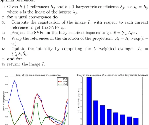
Error of the projection over the sequence
2Ref 3Ref 4Ref
2 Refs 3 Refs 4 Refs 5 Refs 6 Refs 7 Refs 8 Refs 9 Refs
Number of References of the Subspace
0.0 0.2 0.4 0.6 0.8 1.0 1.2 1.4 1.6
Mean Norm of the projection
Error of the projection of a sequence to the Barycentric Subspace
Figure 3: (Left): Example of the norm of the projection vector to the Subspace for 1 patient over the cardiac sequence with 1D, 2D and 3D−Barycentric Subspace. The projection is null for each of reference frames. (Right): Mean norm over all the frame of the sequences and averaged over all the patients for subspaces of increasing number of references.
3. Cardiac Motion Signature from Low-Dimensional Representation In this section, we compute the low-dimension representation of a set of cardiac sequences within Barycentric Subspaces. We show that the features extracted from the representation define relevant cardiac motion signature cap-turing the main phases of a cardiac cycle. In the last part of this section, we compare these features between two populations and we show that they lead to an efficient discrimination.
3.1. Data
We applied the previously defined methodology to compare the cardiac mo-tion signature using two different populamo-tions. The acquisimo-tion consists of a cine sequence in the short-axis view of steady-state free precession magnetic
0.0 0.2 0.4 0.6 0.8 1.0
Frames of the cardiac sequence normalized by the total number of frames
0 1 2 3 4 5 6 7 8 9 Number of Patients
References Frames (2 references: 1D-Barycentric Subspace) Reference 1 Reference 2
0.0 0.2 0.4 0.6 0.8 1.0
Frames of the cardiac sequence normalized by the total number of frames
0 2 4 6 8 10 12 14 Number of Patients
References Frames (3 references: 2D-Barycentric Subspace) Reference 1 Reference 2 Reference 3
Figure 4: Choice of the optimal references within Barycentric Subspaces of increasing dimen-sionality. (Left): 2 reference images. (Right): 3 reference images.
resonance images of two different groups of subjects. he first group consists of 15 controls adults subjects from the openly available dataset Tobon-Gomez et al. (2013). The second group is made of 10 Tetralogy of Fallot (ToF) patients Mcleod et al. (2015). TOF is a congenital heart defect that is present at birth. These patients all had a full repair early in infancy, resulting in the destruction of the pulmonary valves.
3.2. Methods
The stationary velocity fields vi,j parametrizing the deformations between
each frames of the sequences were computed using registrations with the open-source algorithm LCC-Log Demons Lorenzi et al. (2013). In order to improve the registration accuracy, all the images were resampled as a preprocessing step to have an isotropic resolution in the X, Y, Z spatial directions. We apply the methodology described in section 2.2 and project each of the T frames of the cardiac motion to a Barycentric Subspace of dimension k spanned by k + 1 ref-erences. We build the optimal Barycentric Subspace by choosing the references realizing the minimum of the projection energy as described in Algorithm 2. Figure 3 (left) shows the error of the approximation of the subspace with 2, 3 and 4 references over one sequence for one patient. We see a lower error for frames around the references (for which the projection and the error is null) and a larger error for frames further away from the references. Figure 3 (right) shows the error averaged over all the frames (and averaged for a set of 16 healthy patients) and how it varies when the dimension of the subspace is increased. As with traditional dimension reduction methods, the error decreases rapidly for the first dimensions which explain most of the variability of the data. For the remaining of this section, we will focus more specifically on the 1D/2D sub-spaces as they give a good trade-off between the complexity of the subspace and the accuracy of the low-dimensional representation of the motion.
0.0 0.2 0.4 0.6 0.8 1.0 Frames of the cardiac sequence normalized by the total number of frames0.2
0.0 0.2 0.4 0.6 0.8 1.0 1.2
Value of the coefficient
Barycentric Coefficients (2 references, 1D-barycentric Subspace) Lambda 1 Lambda 2
0.0 0.2 0.4 0.6 0.8 1.0
Frames of the cardiac sequence normalized by the total number of frames 0.4 0.2 0.0 0.2 0.4 0.6 0.8 1.0 1.2
Value of the coefficient
Barycentric Coefficients (3 references, 2D-barycentric Subspace) Lambda 1 Lambda 2 Lambda 3
Figure 5: Curves of the lambda coefficients within Barycentric Subspaces of increasing di-mensionality. Both the mean (plain lines) over the complete population of 25 patients and the +σ and −σ curves (dotted lines) are shown. (Left): 1D-Subspace with 2 reference im-ages. (Center): 2D-Subspace with 3 reference imim-ages. (Right): 3D-Subspace with 4 reference images.
3.3. Optimal References Frames and Barycentric Curves
The frame chosen as optimal references are shown in Figure 4 for the Barycen-tric Subspaces with 2 reference (left) and 3 references (right). In order to de-scribe them, we are going to number them as (#1,#2) and (#1,#2,#3) although we ask the reader to keep in mind that there is no specific order in the defini-tion of the references. For the 2 references (1-D) case (left figure) we see that reference #1 (blue) is chosen as either one of the first frame of the sequence, or one of the last. This value is very consistent with the end-diastolic frame, which is one of the two extreme point of the cycle where the heart is fully relaxed. The reference #2 (red) is always a frame close to a third of the time of the full cardiac cycle, which corresponds closely to the end-systolic time, where the heart is fully contracted. Looking now at the subspace built with 3 references (right), we see that reference #2 (red) corresponding to the ES is still quite consistent, with little changes compared to the 1D case (for all the patients the 2nd reference is either the same for both the 1D and 2D case or differs by just one frame, which is comparable to the variability seen in other methods detect-ing the ES frame Kong et al. (2016)). This confirms that the ES frame is well captured by one reference. For the two other references (#1 in blue and #3 in green), one is at the beginning and can be recognized as one of the ED frame whereas the other one is at the end of the sequence and can be related to the frame corresponding to the diastasis even though it is less consistently defined. The mean barycentric coefficients together with the variation at +/ − 1SD are shown in Figure 5 for the 1D (left) and 2D (right) cases. For the 1D case,
the pattern of the coefficients closely relates to the volume curves, with the λ1
peaking on average at a frame close to the ED and λ2peaking at the ES frame.
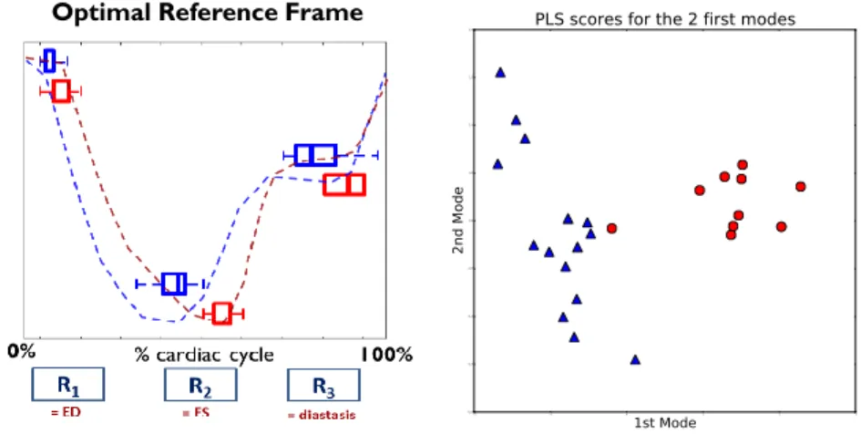
Optimal Reference Frame 2 1 0 1 2 3 1st Mode 2.0 1.5 1.0 0.5 0.0 0.5 1.0 1.5 2.0 2nd Mode
PLS scores for the 2 first modes
Figure 6: (Left): comparison of the optimal references estimated for the healthy controls (blue) and the ToF patients (ref). Significant differences can be seen for the 2nd corresponding to a larger systolic duration. The curves represent two typical patterns of the volume curve for each population. (Right): 2-D plot representing the projection of the two population on the first 2 modes of the PLS. Any linear classifier would be able to separate both populations as two clear clusters appear.
to the ES reference only marginally changes whereas the coefficient which cor-responded to the ED frame is now divided between the 1st and 3rd coefficients at the beginning and end of the cycle.
3.4. Group-Wise Analysis of Differences
Finally, we compare the parameters of each population (healthy vs. ToF) in the case of a 2-D Barycentric Subspace. In the left plot of Figure 6, one can see the difference between the optimal reference frames chosen for each of the population. For the first reference (corresponding to the end-diastole), the frame chosen for each population is quite consistent, with the ToF patients just having a slightly higher value. For the 2nd reference, corresponding to the end-systolic frame, significant differences can be seen between the two populations: the time value of this reference for the ToF population is way higher than the one for the healthy controls. This is a sign that the ToF patients shows higher systolic contraction time, a fact that is confirmed by clinical experience. Reference #3 shows also differences between the two population, with higher intra-population variability.
To investigate further the differences between the two populations, we
per-form a Partial Least Square (PLS) Rosipal and Kr¨amer (2006) decomposition
with the classification (Healthy vs. ToF) as the response variable. PLS decom-poses the data into multiple modes which both explains the variability and the correlation with the response. In our case, the features used were both the 3 optimal reference frames (normalized by the total number of frames) and the 30 barycentric coefficients corresponding to the curves in the 2-D space. For nor-malization, we scale the barycentric coefficients so that their importance in the
Small
deformations deformationsSmall Small
deformations deformationsMedium
Large deformations
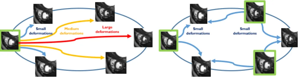
Figure 7: Schematic representation of the proposed approach, references used for each ap-proach are shown in green. Left: traditional apap-proach where only the ED image is used as a reference leading to large displacements to be evaluated between the ED and ES frame. Right: proposed approached where multiple images are used as references, all the images of the sequence are close to at least one reference.
decomposition is similar to the choice of the optimal frames. The projection of the data on a 2-D space can be seen in Figure 6-right. Two clear clusters can be seen, showing that the PLS manages to discriminates the two populations based on the features from the barycentric subspace projection. All these results show that this low-dimensional signature of the motion is encoding relevant features of the cardiac motion.
4. Using Barycentric Subspaces as a prior on the Registration The key instrument of cardiac motion analysis is non-linear registration: it allows to track the motion of the myocardium and compute deformation
fields representing the motion during a cycle. These deformation fields can
then be used to perform statistical analysis and compare different motions. A great variety of registration algorithms Klein et al. (2009) have been developed in medical imaging, some of which have been adapted and improved to the specific task of cardiac motion tracking De Craene et al. (2011). Algorithms whose deformations are parametrized by dense vector fields, for example Beg et al. (2005) provides a generic framework capable of representing any type of deformation of the myocardium at the cost of complexity. In this framework, the direct optimization similarity criterion Sim (measuring the resemblance of two images by comparing voxel intensities) on the whole space of non-parametric transformations leads to an ill-posed problem due to the number of degrees of freedom. To overcome this problem and impose some spatial regularity on the solution, most of the registration methods add a regularization term Reg corresponding to the a priori knowledge one has on the transformation to find. Using the parametrization of the deformations by a SVF v as we introduced in Section 2:
E(v) = Sim(F, M ◦ exp(v)) + Reg(v),
where F is the fixed image, M the moving image. The regularization term can take multiple forms, but most of the time registration algorithms consider slowly
Algorithm 4 Use of the Barycentric Subspace as a prior in the computation of the registration of a frame with respect to k + 1 references.
1: Registration of the image I with respect to k + 1 references Ri.
2: Initialization of the algorithm with the standard registration of the image
with respect to each reference to get v0
i.
3: Compute the projection ˆv0, the coefficients λ
i and the barycentric velocity
fields ˆv0
i such that vi0= ˆv0i + ˆv0 using Algorithm 1.
4: Compute the warped references ˆR0i = Ri◦ exp ˆv0,
5: for j until convergence do
6: Compute the update field ˆuji from each warped reference ˆRj−1i to the
current image I with the demons forces.
7: Project the update field ˆuji to the set of current barycentric velocities ˆvkj−1
and updates the barycentric velocity: ˆvij= ˆvij−1+P
kckvˆ
j−1
k .
8: Compute the warped references ˆRji = Ri◦ exp ˆv
j
i,
9: end for
10: Compute ˆv mapping each warped reference ˆRji to the current image and
compose this SVF with the barycentric velocity to get an estimation of the full deformation: vji = ˆvji + ˆv.
11: Extract the barycentric coefficients such thatP
iλivˆ j
i = 0
12: Return: the estimated barycentric coefficients λiand the k + 1 deformations
vij mapping symmetrically each reference to the image I.
varying deformation as our prior knowledge of the transformation, thereby forc-ing the transformation to be as smooth and as small as possible. This method-ology is efficient to find small deformations, for example the one mapping the ED to nearby frames, but this kind of regularization often leads to an underes-timation of the large deformations as the one happening between the ED and ES frame (see Fig. 7 for a schematic representation).
To correct this bias, one possible solution is to perform the registration in a group-wise manner where a group of images are simultaneously considered and an additional criteria is set up to ensure temporal-consistency Balci et al. (2007). We could use multiple images as references and perform registration so that the reference is close to the frame analyzed (see Fig. 7). But there is now another problem to be dealt with: the registration of each frame being done with respect to a different reference, there is no a common framework and space to analyze the cardiac motion as a whole. In order to have something comparable for all the references, we proceed differently: instead of performing the registration with respect to one image - the closest reference - we build a subspace containing these references and use it as a prior on the registration process.
To do so, we propose to use the barycentric template defined by 3 reference frames of the sequence as the additional prior on the transformations. Instead of applying the regularization energy Reg(v) to the full deformation v, we compute
Frame
0 5 10 15 20 25 30
Average Point-to-point error deformed meshes (mm) 0
0.5 1 1.5 2 2.5 3 3.5 4
4.5 Error of Standard and Barycentric registration
Standard R1 Standard R2 Standard R3 Barycentric R1 Barycentric R2 Barycentric R3 Frame 0 5 10 15 20 25 30 Volume (ml) 50 55 60 65 70 75 80 85 90 95 100
Volume curve Standard and Barycentric registration
Standard Barycentric Ground Truth
Figure 8: (Left): Average point-to-point error on the meshes over the whole cycle between the ground-truth and the deformed meshes compared for the two methods (our proposed approach in dotted lines, and the standard one in plain lines). The registration is performed with respect to the three references for both cases. (Right): volume curves induced by the registration and comparison with the ground truth volume. Our proposed approach (red -dotted) performs a better approximation of the ground truth volume curve (green).
only to this reduce portion of the full deformation. This SVF encodes the dis-tance of the image to the subspace and is smaller that the full deformation (see Figure 2 ). By relaxing the regularization this way, we let the registration move freely within the a 2-D barycentric template representing the cardiac motion. 4.1. Barycentric Log-Demons Algorithm
The methodology defined is quite generic, we detail in this section one way to implement it in practice in the case of the LCC Log-Domain Diffeomorphic Demons algorithm Lorenzi et al. (2013). This algorithm proceeds in multiple iterations of two successive steps: the first step optimizes the matching criteria by computing the so-called demons forces, then, in the second step, the esti-mated velocity field is smoothed by applying a Gaussian filter. To allow the registration to freely move in the barycentric subspace defined by a set of im-ages - instead of being constrained by the regularization on the whole velocity field (the ”standard” method) - we proceed in two steps: first we evaluate the barycentric subspace structure and then we iterate on this subspace. To do so, we perform one standard registration of the current image I with respect to
each of the references Ri to get the velocity fields vi. Then, we decompose the
velocity field vi as the sum of the barycentric velocity ˆvi warping the reference
Ri to the projection ˆI inside the barycentric subspace and the residual velocity
field ˆv of the projection (see Fig. 2). Finally, we iterate by projecting the update
demons forces on the barycentric velocity until convergence. The barycentric template is therefore used as a prior on the cardiac motion and we perform the regularization only with respect to the projecting field. The methodology is described in Algorithm 4.
4.2. Evaluation using a Synthetic Sequence
We evaluate the method using one synthetic time series of T = 30 cardiac im-age frames computed using the method described in Prakosa et al. (2013). The use of a synthetic sequence has the important advantage to provide a dense point correspondence field following the motion of the myocardium during the cardiac cycle which can be used to evaluate the accuracy of the tracking. Another op-tion could be to use point correspondence manually defined by experts, but they tend to be inconsistent and not reliable Tobon-Gomez et al. (2013). First, we compute the optimal references using the methodology described in Algorithm 2, giving us the three reference frames spanning the barycentric subspace: #1 is frame 1, #2 is frame 11 and #3 is frame 21. Then we register each frame i of the sequence using the method described above to get the deformations from each of the three references to the current images using both the standard method and our approach using Barycentric Subspaces as a prior. We deform each of the 3 ground truth meshes corresponding to the reference frames (1,11 and 21) with the deformation from the reference frame to the current frame. We compare our approach with the standard approach where the registration between one of the reference and the current frame is done directly. In Figure 8 (left), we show the point-to-point registration error of the deformed mesh using the 3 different deformations (one with respect to each references). Substantial reduction of the error (of about 30%) can be seen for the largest deformations (between end-systole and the first reference for the blue curve corresponding to the frame 1 chosen as reference). This comes at the cost of additional error for the small deformations evaluated at the frame near the respective references. In Figure 8 (right), we show the estimation of the volume curve (which is one of the most important cardiac feature used in clinical practice). Our better estimation of the large deformation leads to a substantial improvement of the volume curve estimation. In particular the estimation of the ejection fraction goes from 32% with the standard method to 38%, closer to the ground truth (43%), reducing the estimation error by half.
4.3. Towards Symmetric Transitive Registration
Traditionally in cardiac motion tracking, two different method for computing the motion deformations can be used. The first method, which we have seen in the previous section, estimates the motion by computing the deformation from each frame to a common reference. The second method computes the deformation mapping each successive frame and then derive the full motion by composing these deformations one by one. The problem encountered by
most registration algorithms in this context is the lack of transitivity ˇSkrinjar
et al. (2008): the deformation given by the registration between two images is different when it is done directly or by the composition of the result of the registration with an intermediate image (in our setting this condition can be
written as vij = BCH(vk i, v j k) ' v k i + v j
k: this is an approximation using the
BCH decomposition at the first order as was done before in this paper). This is due to the accumulation of the registration errors at each step of the registration and can lead to large errors at the end of the cycle.
BARYCENTRIC SUBSPACE
Image
0 5 10 15 20 25 30
Frames of the cardiac sequence 0.0 0.5 1.0 1.5 2.0 2.5 3.0
Average point-to-point error of the deformed meshes
Error of frame-to-frame registration
Standard Transitive Barycentric
Figure 9: (Left): Schematic representation of the symmetric multi-references barycentric registration in the case of a 1-D barycentric subspace spanned by 2 references. Itand Isare two
frames of the sequence and ˆIt, ˆIscorresponds to the respective projection to the barycentric
subspace. (Right): comparison of the error between the standard registration (blue plain), the barycentric method presented in section 3.1 (blue dotted) and the symmetric-barycentric extension presented in section 3.2 (red dotted).
In this last section, we use the barycentric subspace representation to derive a method to get approximately transitive registration (at the first-order of the BCH approximation), an important property of the registration ensuring ro-bustness. This method is schematically represented in Figure 9 in the case of a Barycentric Subspace with 2 references.Using Barycentric Subspaces as a basis for the registration at each step, we define the symmetric registration using the following formula 1 which is schematically represented in Fig. 9 (left):
Wst= ˆvs− ˆvt+ 1/2(X
i
λtiˆvis−X
i
λsivˆti). (1)
The equations leading to this formula are detailed in Appendix B, and we will only give here a simple interpretation of the meaning of the formula. The first two SVFs on the left represent the residual projections from the barycentric subspace to the two frames. This encodes what cannot be represented in the
subspace. The sum on the right is a symmetric estimation of the SVF ˆWt
s
(the vector representing the deformation from the projection of one image to the other one) within the barycentric subspace. This estimation is done by going through each reference image forward and backward and weighting the barycentric velocity by the coefficients on the subspace. We apply it to frame-to-frame registration and show a significant improvement of the accuracy of the registration with respect to a non-transitive method. In figure 9 (right), the error for frame-to-frame registration (starting for frame 0) of our method compared with the standard one can be seen. Even though our method has higher error for the first frames of the sequence, the transitivity property ensures that there is not an accumulation of the error for the last frames of the sequence as opposite to the traditional method, meaning that we have substantially less error for frames wt the end of the cycle.
Figure 10: Reconstructed sequences using the barycentric representation compared with other methods. (Top row): initial true cardiac sequence. (Second row): reconstruction using PCA decomposition with the ED frame as reference. (Third row): reconstruction using PCA with the mean image as reference. (Bottom row): proposed approach using Barycentric compact representation of the motion. Each column corresponds to one frame of the sequence which are from left to right: 0 (ED), 5, 10 (ES), 15, and 25.
5. Reconstruction of Cardiac Sequences
In this section, we evaluate the reconstruction of the sequence using our low-dimensional representation. From one sequence of 30 cardiac images we compute the Barycentric coefficients and reference frames using the previously defined methodology. Then we reconstruct the sequence simply using these coefficients (3 coefficients for each frame) which represent the position of each frame in the 2-D Barycentric subspace - and the 3 reference images. We compare our method with two single reference approaches. The first one, we start from the ED image and we perform the PCA covariance analysis on the tangent vectors of the deformations. We build a 2-D subspace by taking the first two modes of the PCA decomposition. The cardiac motion is reconstructed by applying this low-dimensional representation of the deformation to the ED image. The second one, the same methodology is applied but with the analysis done at the mean image computed using all the images of the sequence. To sum up, both these methods are encoded by the scores of the 2 modes, 1 scalar image for the reference (the ED frame for the first method or the mean for the second) and 2 vector images representing the coefficients of the modes.
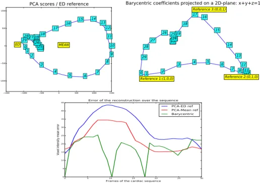
1500 1000 500 0 500 1000 1500 1000 500 0 500 1000 01 2 3 4 5 6 7 8 9 10 11 12 13 14 15 16 17 18 19 20 212223 24 25 26 27 28 29 ED MEAN
PCA scores / ED reference
0 1 2 3 4 5 6 7 8 9101211 13 14 15 16 17 18 19 20 21 22 2324 25 26 27 28 29 Reference 1:(1,0,0) Reference 2:(0,1,0) Reference 3:(0,0,1)
Barycentric coefficients projected on a 2D-plane: x+y+z=1
0 5 10 15 20 25 30
Frames of the cardiac sequence
0 5 10 15 20 25 30 35 40 45
Voxel intensity mean error
Error of the reconstruction over the sequence PCA-ED ref PCA-Mean ref Barycentric
Figure 11: (Top): comparison of the 2-D representation of single reference PCA versus multi-reference Barycentric. (Bottom): Error of the reconstruction of the sequence for the different methods.
5.1. Qualitative results
A qualitative comparison of the different methods can be seen in Figure 10. PCA with the ED image as reference (2nd row) performs a good reconstruction for the early frame of the sequence but fails to reconstruct well the large defor-mation of the ES (3rd column) compared to the initial sequence (1st row): the fact that there is only one reference image limits its ability to update the change of appearance of the images during the cardiac cycle. PCA at the mean image (3rd row) performs betters to recover these frames, but the overall appearance of the image is blurred because the initial texture is not defined using a single frame but an average of images. Finally, our proposed approach using multiple references (4th row) has a similar appearance to the initial sequence for all the frames of the cycle.
5.2. Quantitative results
A quantitative comparison of the performance of the three methods is shown in Figure 11. Top figures show a comparison of the 2-D PCA (with ED image as reference) and Barycentric low-dimensional representation. The chosen refer-ence frames for the Barycentric methods are referrefer-ence #1 is frame 0, referrefer-ence #2 is frame 10 and reference # 3 is frame 17 and represent the different phases
of the cycle. For the PCA method, there is only one reference which only ac-count correctly for the part of the motion close to this single reference. We can also see that the PCA curve never gets close to the mean point (coordinates 0,0) which is therefore a poor descriptor of the motion. Finally, the mean voxel intensity error with respect to the initial sequence, Figure 11 (bottom), shows a better performance of the multi-reference Barycentric approach than for the traditional PCA (reduction of the error on average of approx 30%).
6. Conclusion
In this paper, we have challenged the traditional framework for studying the cardiac motion based on the ED frame chosen as the single reference. In-stead, we have proposed a multi-references methodology introducing a new type of subspaces called Barycentric Subspaces. Intuitively, this multi-reference ap-proach is more adapted to the cardiac motion circular pattern and overcomes the drawback of having either to chose one specific template such as the ED frame (whose choice might introduce bias) or to compute a mean image (which might be a poor descriptor of the whole distribution). The practical methods and algorithms to use these subspaces in the context of the manifold of medical images have been derived: how to compute the projection and the coefficients of a specific image and how to compute an image from the coefficients. We have presented three possible applications where this framework show clear ad-vantages over the traditional method. The first application is the computation of a low-dimensional representation of the cardiac motion from the projection on to the subspace leading to an efficient discrimination between two popula-tions of healthy and diseased patients. Then, we have shown on to introduce these subspaces as an additional prior within a registration algorithm to re-lax the regularization constraint. Finally, we have compared the reconstruction of the sequence using our multi-reference low-dimensional representation with traditional representation using one reference.
In the context of cardiac motion, this new approach could also provide a consistent framework to perform a longitudinal study of the motion during a therapy or the evolution of a disease. Also, the results shown for the recon-struction and the comparison with the first-reference methods are promising and could be extended to build a multi-references methodology to synthesize cardiac sequences of images and extend the existing single reference approaches Prakosa et al. (2013). Finally, the multi-reference approach introduced in this work might be applied to medical imaging problems going beyond the scope of cardiac motion. Because of the generality of the methods which were defined for any set of images, an extension to define a new generic framework for multi-atlas approaches applied to any type of medical images might be possible.
Acknowledgments. The authors acknowledge the partial funding by the EU FP7-funded project MD-Paedigree (Grant Agreement 600932)
Appendix A. Projection of an image to the Barycentric Subspace Starting from the optimization problem defined in 2.2:
min ˆ v k ˆv k 2, subject toX i λi(vi− ˆv) = 0, X i λi6= 0.
Without loss of generality, we can add the additional condition that the λ should
sum to one: P
iλi = 1. We also add the constraint λi ≤ 1. keeping in mind
that what follows can be easily extended to the unconstrained case. Then, the optimization becomes: min ˆ v k ˆv k 2, subject to v =ˆ X i λivi, X i λi= 1, λi≤ 1,
whose Lagrangian is:
L(λ, µ, κ) =kX i λivik2+µ(1 − X i λi) + κ(1 − λ),
where κ and λ are vectors, µ is scalar. The solution can be found by solving the set of equations Bertsekas (2014):
∀j : hP iλivi|vji = (µ + κj)/2 ∀j : κj(1 − λj) = 0 ∀j : κj ≥ 0 P iλi = 1.
If all κi are equal to zero, which is equivalent to the inequality constraint not
being filled, then we simply have to solve : hP
iλivi|vji = µ for all j. Denoting
S the matrix of the scalar product Si,j = hvi|vji, this is equivalent to:
Sλ = µ1.
Finally adding the conditionP
iλi= 1 gives us the optimal solution λ∗:
λ∗= S−11/X
i
(S−11)i.
If some κi are not null, then λi = 1 for these indices. We simply have to solve
the lower-dimensional problem removing the satisfied inequality constrains.
Appendix B. Frame-To-Frame Barycentric Registration Formulation
Given two images Itand Is, images of a cardiac sequence at frame number t
and s, we want to derive the formula for the SVF Ws
t mapping one image to the
other using their projection on to the barycentric subspace. We use the notation
map the projections ˆIs and ˆIt, ˆvs will be the projection of one frame s to the
subspace, vsi will be the SVF mapping the image to the reference i and ˆvsi will
the the SVF mapping the projected image to the reference.
Using a BCH approximation at the first order, we have the following equality with is true with respect to each reference i:
ˆ
Wst= BCH(ˆvsi, −ˆvit) ≈ ˆvsi − ˆvit.
Taking the λ-weighted sum and using the fact thatP
iλ s iˆv s i = 0 and P iλ t iˆv t i = 0
give us the two following equalities: ˆ Wst= X i λtiˆv s i = − X i λsivˆ t i.
Finally, we take the average of these two equalities and add the projection vector to get our frame-to-frame formulation of the registration using the subspace:
Wst= ˆvs− ˆvt+ 1/2(X i λtiˆvis−X i λsivˆti). References
Balci, S.K., Golland, P., Wells, W., 2007. Non-rigid groupwise registration
using b-spline deformation model. Open source and open data for MICCAI , 105–121.
Beg, M.F., Miller, M.I., Trouv´e, A., Younes, L., 2005. Computing large
defor-mation metric mappings via geodesic flows of diffeomorphisms. International journal of computer vision 61, 139–157.
Bertsekas, D.P., 2014. Constrained optimization and Lagrange multiplier meth-ods. Academic press.
Bijnens, B., Claus, P., Weidemann, F., Strotmann, J., Sutherland, G., 2007. Investigating cardiac function using motion and deformation analysis in the setting of coronary artery disease. Circulation .
De Craene, M., Tobon-Gomez, C., Butakoff, C., Duchateau, N., Piella, G., Rhode, K.S., Frangi, A.F., 2011. Temporal diffeomorphic free form deforma-tion (tdffd) applied to modeforma-tion and deformadeforma-tion quantificadeforma-tion of tagged mri sequences, in: International Workshop on Statistical Atlases and Computa-tional Models of the Heart, Springer. pp. 68–77.
Fletcher, P.T., Lu, C., Pizer, S.M., Joshi, S., 2004. Principal geodesic analysis for the study of nonlinear statistics of shape. IEEE transactions on medical imaging .
Hammer, Ø., Harper, D., Ryan, P., 2009. Past-palaeontological statistics, ver. 1.89. University of Oslo, Oslo , 1–31.
Joshi, S., Davis, B., Jomier, M., Gerig, G., 2004. Unbiased diffeomorphic atlas construction for computational anatomy. NeuroImage .
Klein, A., Andersson, J., Ardekani, B.A., Ashburner, J., Avants, B., Chiang, M.C., Christensen, G.E., Collins, D.L., Gee, J., Hellier, P., et al., 2009. Eval-uation of 14 nonlinear deformation algorithms applied to human brain mri registration. Neuroimage 46, 786–802.
Kong, B., Zhan, Y., Shin, M., Denny, T., Zhang, S., 2016. Recognizing end-diastole and end-systole frames via deep temporal regression network, in: In-ternational Conference on Medical Image Computing and Computer-Assisted Intervention, Springer. pp. 264–272.
Konstam, M.A., Kramer, D.G., Patel, A.R., Maron, M.S., Udelson, J.E., 2011. Left ventricular remodeling in heart failure. current concepts in clinical sig-nificance and assessment. JACC: Cardiovascular Imaging .
Lorenzi, M., Ayache, N., Frisoni, G.B., Pennec, X., 2013. LCC-Demons: a robust and accurate symmetric diffeomorphic registration algorithm. Neu-roImage 81, 470–483.
Mcleod, K., Sermesant, M., Beerbaum, P., Pennec, X., 2015. Spatio-Temporal Tensor Decomposition of a Polyaffine Motion Model for a Better Analysis of Pathological Left Ventricular Dynamics. IEEE Transactions on Medical Imaging 34, 1562–1675.
Pennec, X., 2015. Barycentric Subspaces and Affine Spans in Manifolds, in: Geometric Science of Information GSI’2015, Second International Conference, Palaiseau, France.
Prakosa, A., Sermesant, M., Delingette, H., Marchesseau, S., Saloux, E., Al-lain, P., VilAl-lain, N., Ayache, N., 2013. Generation of Synthetic but Visually Realistic Time Series of Cardiac Images Combining a Biophysical Model and Clinical Images. IEEE Transactions on Medical Imaging 32, 99–109.
Qiu, A., Younes, L., Miller, M.I., 2012. Principal component based diffeomor-phic surface mapping. IEEE transactions on medical imaging 31, 302–311.
Rao, A., Sanchez-Ortiz, G.I., Chandrashekara, R., Lorenzo-Vald´es, M.,
Mohi-addin, R., Rueckert, D., 2003. Construction of a cardiac motion atlas from mr using non-rigid registration, in: International Workshop on Functional Imaging and Modeling of the Heart, Springer. pp. 141–150.
Roh´e, M.M., Duchateau, N., Sermesant, M., Pennec, X., 2015. Combination
of Polyaffine Transformations and Supervised Learning for the Automatic Diagnosis of LV Infarct, in: Statistical Atlases and Computational Modeling of the Heart (STACOM 2015), Munich, Germany.
Roh´e, M.M., Sermesant, M., Pennec, X., 2016. Barycentric Subspace Analy-sis: a new Symmetric Group-wise Paradigm for Cardiac Motion Tracking, in: MICCAI 2016 - the 19th International Conference on Medical Image Com-puting and Computer Assisted Intervention, Athens, Greece. pp. 300–307.
Rosipal, R., Kr¨amer, N., 2006. Overview and recent advances in partial least
squares, in: Subspace, latent structure and feature selection. ˇ
Skrinjar, O., Bistoquet, A., Tagare, H., 2008. Symmetric and transitive regis-tration of image sequences. Journal of Biomedical Imaging .
Sweet, A., Pennec, X., 2010. Log-domain diffeomorphic registration of diffusion tensor images, in: International Workshop on Biomedical Image Registration, Springer. pp. 198–209.
Tobon-Gomez, C., De Craene, M., Mcleod, K., Tautz, L., Shi, W., Hennemuth, A., Prakosa, A., Wang, H., Carr-White, G., Kapetanakis, S., Lutz, A., Rasche, V., Schaeffter, T., Butakoff, C., Friman, O., Mansi, T., Sermesant, M., Zhuang, X., Ourselin, S., Peitgen, H.O., Pennec, X., Razavi, R., Rueckert, D., Frangi, A.F., Rhode, K., 2013. Benchmarking framework for myocardial tracking and deformation algorithms: an open access database. Medical Im-age Analysis 17, 632–648.
Vaillant, M., Miller, M.I., Younes, L., Trouv´e, A., 2004. Statistics on
diffeomor-phisms via tangent space representations. NeuroImage 23, S161–S169. Vercauteren, T., Pennec, X., Perchant, A., Ayache, N., 2008. Symmetric
log-domain diffeomorphic registration: A demons-based approach, in: Metaxas,
D., Axel, L., Fichtinger, G., Sz´ekely, G. (Eds.), Proc. Medical Image
Com-puting and Computer Assisted Intervention (MICCAI’08), Part I, Springer, New York, USA. pp. 754–761.
Zhang, M., Wells III, W.M., Golland, P., 2016. Low-dimensional statistics
of anatomical variability via compact representation of image deformations, in: International Conference on Medical Image Computing and Computer-Assisted Intervention, Springer. pp. 166–173.