Algorithms and Low-Power Hardware for Image
Processing Applications
by
Alex Ji
BASc in Engineering Science,.University of Toronto (2016)
Submitted to the Department of Electrical Engineering and Computer
Science
in partial fulfillment of the requirements for the degree of
Master of Science in Electrical Engineering and Computer Science
at the
MASSACHUSETTS INSTITUTE OF TECHNOLOGY
June 2018
@
Massachusetts Institute of Technology 2018. All rights reserved.
Signature redacted
A uthor ... ... '... . **. . . .. . . ....
Department of Electrical Engin ering and Computer Science
May 25, 2018
Signature redacted
C ertified by ...
..
Anantha P. Chandrakasan
Vannevar Bush Professor of Electrical Engineering and Computer Science
Thesis Supervisor
Accepted by
...
ignature
redacted
MASS HUSETS YTITUTE Leslie AjAf4odziejski
OF TECHNOLOGY eleA odijk
Professor of Electrical Engineering and Computer Science
JUN 18 2018
Chair, Department Committee on Graduate Students
Algorithms and Low-Power Hardware for Image Processing
Applications
by
Alex Ji
Submitted to the Department of Electrical Engineering and Computer Science on May 25, 2018, in partial fulfillment of the
requirements for the degree of
Master of Science in Electrical Engineering and Computer Science
Abstract
Image processing has become more important with the ever increasing amount of available image data. This has been accompanied by the development of new algorithms and hardware. However, dedicated hardware is often required to run these algorithms efficiently and conversely, algorithms need to be developed to exploit the benefits of the new hardware. For example, depth cameras have been created to add a new dimension to human-computer interaction. They can benefit applications that can operate on the raw depth data directly, such as breath monitoring. As for new algorithms, convolutional neural networks (CNNs) have become the standard for difficult image processing tasks due to their high accuracy. But to execute them efficiently, we need new hardware to fully exploit the parallelism inherent in these computations.
The first part of the thesis presents an algorithm for breath monitoring using a low-resolution time-of-flight camera. It consists of automatic region-of-interest detection, followed by frequency estimation. It can be accurate to within 1 breath per minute, comparing with a respiratory belt as reference.
The second part presents a processing element (PE) for a neural network accelerator supporting compressed weights and using a new technique called factored computation. The PE consists of an accumulator array, row decoder, and output combination block. Modifications to the row decoder can allow for reconfigurability of the compressed weight bit-widths.
Several common layer operations in CNNs are described and mapped onto the proposed hardware. An energy model of the design is formulated and verified by synthesizing and simulating a basic processing element containing an 8 x 20 accumulator
array. Simulations show the proposed design achieves up to 4.5 x reduction in the energy per MAC compared to a baseline 16-bit fixed-point MAC unit.
Thesis Supervisor: Anantha P. Chandrakasan
Acknowledgments
First, I would like to thank Prof. Anantha Chandrakasan for his guidance, support, and patience. He has given me the freedom to explore many different topics, always aiming to find the one that would excite me the most. This has exposed me to areas I never would have thought I would get to work on.
Next, Wanyeong has been a great help throughout this process. As the lead of the machine learning project, he has kept the project moving smoothly with his detailed planning. I can always rely on him to discuss any new ideas or questions I might have. I also appreciate him taking the time to review and provide insightful comments on several drafts of this thesis.
I would also like to thank Prof. Song Han for finding time in his busy schedule to meet with us and provide us with valuable feedback on our ideas.
I would like to acknowledge TSMC for their funding for the machine learning project and Shih-Lien for consistently providing us with useful comments and ideas during our biweekly phone calls.
My graduate school experience thus far has been made all the more enjoyable by the collaborative atmosphere of AnanthaGroup. In particular, I would like to thank Priyanka, Mehul, Chiraag, Utsav, and Mohamed for helping me prepare for presentations and for their technical support.
Contents
1 Introduction
1.1 Time-of-Flight Breath Monitor . . . .
1.1.1 Existing Methods for Breath Monitoring and Related Research
1.2 Machine Learning Processor . . . . 1.2.1 Existing Neural Network Accelerators . . . . 1.2.2 Compression and Quantization Schemes . . . .
1.2.3 Overview of Proposed Design . . . .
2 Breath Monitor Using Time-of-Flight Imaging
2.1 Algorithm for Breathing Rate Extraction . . . . 2.1.1 Automatic Region-of-Interest Detection . 2.1.2 Frequency Estimation . . . . 2.2 R esults . . . . 2.2.1 Test Setup . . . . 2.2.2 ROI Detection. . . . . 2.2.3 Accuracy . . . . 2.2.4 Summary . . . .
3 Efficient Processing Element Architecture Supporting Compressed Weights
3.1 Factored Computation . . . . 3.2 Performing General Fixed-Point Computations . . . . 3.3 Mapping to Hardware . . . . 11 12 12 14 14 18 20 21 21 21 25 27 27 28 30 30 33 33 36 37 . . . . . . . .
3.3.1 General Hardware Structure . . . . 37
3.3.2 Flexibility . . . . 38
4 Dataflow in the Proposed Architecture 41 4.1 O verview . . . . 41
4.2 Mapping Operations onto the Processing Element . . . . 41
4.2.1 Depthwise Convolutions . . . . 42
4.2.2 Pointwise (1 x 1) Convolutions . . . . 44
4.2.3 General Convolutions . . . . 48
4.2.4 Fully-Connected Layers . . . . 50
4.3 Sum m ary . . . . 53
5 Energy Model and Simulations 55 5.1 Relation to Accumulator Array Dimensions . . . . 55
5.2 Form ulation . . . . 56
5.3 Simulation Flow . . . . 60
5.4 Accumulator Input Gating . . . . 61
5.5 Basic Processing Element . . . . 63
6 Conclusion and Future Directions 67 6.1 ToF Breath Monitor . . . . 67
List of Figures
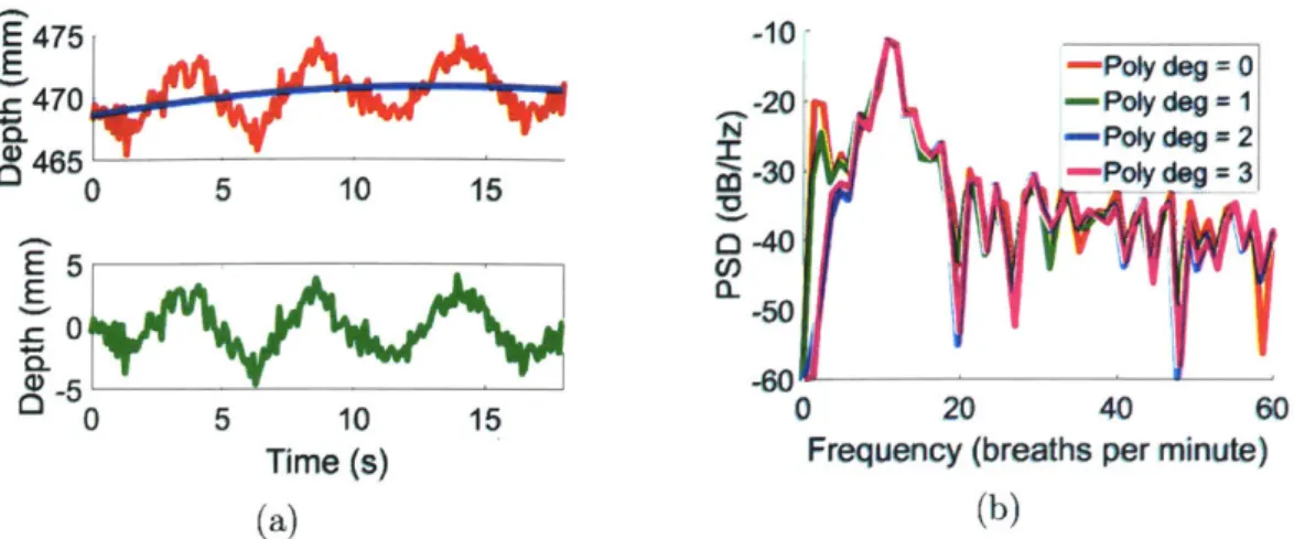
2-1 Breathing rate extraction algorithm: (1) ROI detection, (2) average depth extraction, and (3) frequency estimation. . . . . 22 2-2 (a) Average depth data with quadratic fit (top) and detrended version
(bottom). (b) Effect of detrending with different degrees of polynomials in the frequency domain. . . . . 23 2-3 Histogram of peak frequency bins for each pixel. . . . . 24 2-4 Block diagram of FPGA implementation of automatic ROI detection. 25 2-5 Erroneous peak detection on noisy data. . . . . 26 2-6 Quadratic interpolation of frequency peak. Figure from [1]. . . . . 27 2-7 Block diagram of FPGA implementation of frequency estimation. . . 28 2-8 GUI used for system testing. . . . . 29 2-9 Automatically selected ROI (ROI size = 300 pixels) from various
sub-jects with the breathing signal concentrated in (a) both the chest and abdomen, (b) mainly the abdomen, and (c) mainly the chest. . . . . . 29 2-10 Automatically selected ROI, with an ROI size of (a) all valid pixels, (b)
300 pixels, and (c) 50 pixels. . . . . 30 2-11 Sample results of final estimated breathing rate, along with reference
sign al. . . . . 3 1 3-1 (a) Typical computation method: multiplication and weight look-up
are performed before each accumulation. (b) Alternative computation method: multiplication and weight look-up are performed after all accumulations are completed. . . . . 35 3-2 (a) PE structure [2]. (b) Accumulator group. . . . . 39 4-1 Dataflow for a depthwise (2-D) convolutional layer mapped onto a 3 x 4
accumulator array. The array is shown on the left while the portion of the computation being performed is highlighted on the right. . . . . . 45 4-2 Dataflow for a 1 x 1 convolutional layer mapped onto a 3 x 4 accumulator
array . . . . 47 4-3 Dataflow for a general convolutional layer mapped onto a 3 x 4
accu-m ulator array. . . . . 51 4-4 Dataflow for a FC layer mapped onto a 3 x 4 accumulator array. . . . 54 5-1 Accumulator array with labeled dimensions. Each square represents an
5-2 Detailed simulation flow. . . . . 60 5-3 (a) Accumulator with input gating. (b) Accumulator without input
gating. (c) Timing diagram. . . . . 61 5-4 Average energy per accumulation (EAcc) vs. average number of cycles
between accumulations (TAcc) with gated (solid) and ungated (dotted) inputs. . . . . 62 5-5 Normalized energy per MAC (EMAc) vs. number of accumulations
performed in each accumulator group before output combination (NAcc). 64
5-6 Number of MACs performed per output pixel (left axis) and total number of MACs per layer (right axis) in different layers of (a) AlexNet, (b) VGG-16, and (c) MobileNet. . . . . 65
Chapter 1
Introduction
Automated image processing can benefit and in some cases, is essential to many applications including medical diagnosis, self-driving cars, and wearable navigation. They often utilize image recognition or object detection techniques. This has been made possible by the recent advances in computer vision. These complex image processing tasks face some common challenges, which include the need for (1) better sensing methods, (2) simpler, or more accurate algorithms, and (3) more energy-efficient processing. Note that these challenges are not independent. Capturing the data in a more suitable form for computation will naturally simplify the algorithms, and having less noise in the data will help improve the accuracy of the algorithms. Having simpler algorithms will reduce the amount of computation involved, making it less demanding for the hardware. Conversely, having efficient hardware would allow more complex algorithms to be executed. Overcoming these challenges would lead to low-power, low-cost implementations of systems leveraging powerful image processing techniques.
This thesis aims to address these challenges for two separate applications. The first uses time-of-flight (i.e. depth) imaging to develop simple algorithms for breath monitoring. This focuses on the second challenge of creating simple, accurate
al-gorithms, by taking advantage of improved sensing methods. The second involves designing a general-purpose machine learning accelerator capable of running the newest convolutional neural network architectures, with a focus on supporting compressed weights and reconfigurable bit-widths. This addresses the third challenge of more
efficient processing hardware.
1.1
Time-of-Flight Breath Monitor
Breathing is a physiological signal that can be useful in medical diagnosis, health tracking, as well as sleep and baby monitoring. Rapid, shallow breathing could be a symptom of diseases such as asthma or pneumonia. For everyday tracking, it can be an indicator of well-being. Slow, steady breathing could be associated with calmness, while quick breathing could reflect tension or anxiety. For sleep monitoring, breathing rate could be used to detect sleep apnea, and also distinguish between rapid eye movement (REM) sleep (marked by irregular breathing patterns) and non-REM sleep (marked by more regular breathing). For baby monitoring, a sudden drop in breathing rate could be one of the first indicators of sudden infant death syndrome.
1.1.1
Existing Methods for Breath Monitoring and Related
Research
In clinical settings, current methods for measuring breathing rate involve the patient breathing into an apparatus (e.g. a spirometer) or placing sensors on their body (e.g. on a belt). Besides being potentially obstructive, these methods could alter the breathing of the patient, resulting in unrepresentative measurements. To handle this, we need a breath monitoring system that is non-contact, but still achieves similar or better accuracy compared to existing methods.
cameras are a type of depth camera that measure depth by emitting modulated infrared (IR) light onto the scene and measuring the phase difference between the transmitted and received light. The active IR illumination allows the system to work well in dark or low-light situations, but consumes a large fraction of the total system power.
Other related work include systems using radio waves [3] and motion magnification of RGB videos [4]. These approaches generally work well, achieving good correlation with reference values, but are computationally intensive. In the case of radio waves, phenomena such as multiple reflections need to be taken into account. Motion magnification requires the computation of complex pyramid-based transforms. In addition, motion magnification of RGB videos has difficulty operating in the dark, making it unsuitable for use in sleep monitoring.
In contrast, algorithms for breath monitoring using depth cameras are quite simple because the breathing signal can be extracted almost directly from the raw depth data [5][6]. The typical approach involves manually selecting the region containing the breathing motion (i.e. the chest and/or abdomen), averaging the depth values in that region, and then extracting the breathing rate using either peak detection or Fast Fourier Transform. Alinovi et al. use an automatic region-of-interest (ROI) detection technique along with large motion detection to identify when to recalculate the ROI [7]. These works use cameras such as the Microsoft Kinect that consume on the order of 1 to 10 W. It is difficult to incorporate these into portable systems that can run on batteries for a reasonable length of time. Instead, we target a low-power low-resolution ToF camera from Texas Instruments (TI OPT8320) that only consumes several hundred mW.
1.2
Machine Learning Processor
In recent years, convolutional neural networks (CNNs) have rapidly gained popularity due to their ability to achieve high accuracy in difficult tasks such as image classification. However, these networks require a substantial amount of computation to process just one image and a large amount of storage for the fixed weight parameters and intermediate results. This is why execution of these tasks are generally done on the cloud. However, this approach has issues with latency, power, and security. This could be an issue for applications that require real-time performance, such as self-driving vehicles. Connection reliability and latency variation to the remote server can also be critical. The power consumption is high because the computations are run on high-performance processors such as GPUs. The power for data transfer can also be significant depending on the application. Security is a concern because it may not be desirable to send private data to the cloud. Instead, it would be more secure if the main processing is done on the edge device itself and only the relevant information is transferred.
It is also possible to run these computations on devices like mobile GPUs, but this typically consumes over 1 W of power, which would quickly drain the battery in just a few hours. For IoT devices which may not have such powerful processors, performing these computations may not be even feasible. Using a dedicated hardware accelerator for these tasks has the potential to reduce the power consumption by at least an order of magnitude.
1.2.1
Existing Neural Network Accelerators
There has been extensive research on designing accelerators for neural networks. The following are just a sample of the wide range of accelerators that have been designed in the past few years. Recent trends include increased reconfigurability to support
variable precision and compressed data. However, the majority of these works do not include how the reduced precision affects the overall accuracy of the networks in their performance metrics. Also, some of these works focus on only one type of computation (e.g. only fully-connected layers or only convolutional layers). But it is important to be able to support all the operations required by neural networks in order to create a general processor capable of running existing networks and also newer networks entirely on-chip.
The majority of the accelerators presented below process a pair of weights and activations at a time. This provides maximum flexibility, but more parallelism is possible by broadcasting inputs and activations across multiple MAC elements at the same time, as in ENVISION [8]. This array-like structure benefits convolutional layers, but could suffer from lower utilization and energy overhead for other layers with less data reuse (e.g. fully-connected layers). EIE supports compressed weights, but only for fully-connected layers
[9].
UNPU (and its predecessor, DNPU) implement LUT-based multiplier structures to achieve some energy savings due to activation and weight reuse [10][11]. A comparison of these accelerators is shown in Table 1.1.Eyeriss
Eyeriss is an accelerator employing a spatial architecture with a 14 x 12 array of processing elements (PEs) and a large 108 kB global buffer. The focus is on efficiently running convolutional layers as these make up the majority of computations in state-of-the-art CNNs. They introduce a new dataflow called row stationary that minimizes overall energy by optimizing across all forms of data reuse. Each PE processes a row of input activations and a row of filter weights. PEs performing computations on the same output channel are grouped together into a logical PE set. Within a logical PE set, filter weights are reused across a row of PEs, input activations are reused along the diagonal, and output partial sums are accumulated vertically. These logical PE
Table 1.1: Comparison table of existing neural network accelerators. The layer types described are convolutional layers (CL), fully-connected layers (FC), and recurrent layers (RL). N/R indicates values that are not reported.
Eyeriss EIE [9] ENVISION [8]
UNPU [10]
____ ____ ___ ___ [12]
Layers supported CL, FC FC only CL only CL, FC, RL Technology 65 nm 45 nm 28 nm FD-SOI 65 nm Supply voltage 1 N/R 1 1.1 [V] Clock frequency 200 800 200 200 [MHz] Power [mW] 278 600 44 297 Area [mm2] 16 40.8 1.9 16 4, 8, 16 16 (4-bit (activations and
Precision [bits] 16 compressed) weights scaled (weights), 16
together) (activations) Energy per
classification 8.0 0.032 0.94
N/R (AlexNet) (FC only) (CL only)
[mJ/frame]
sets are then mapped onto the physical PE array.
EIE
Efficient Inference Engine (EIE) provides a hardware implementation for the deep compression algorithm (see Section 1.2.2) [9]. It is designed to efficiently process fully-connected layers, so it does not exploit much data reuse. Instead, the focus is on taking advantage of weight compression and data sparsity (for both weights and activations) to significantly reduce the amount of memory accesses and computations.
The rows of the weight matrix, output vector, and input activations are uniformly distributed across multiple PEs. The PEs perform a hierarchical leading non-zero detection on the input activations to find the non-zero entries. The non-zero activations and their indices are then broadcast to all the PEs. Each of these activations is multiplied by the non-zero entries in the corresponding column of the weight matrix and
the products are stored in the appropriate output entry. Hence, only multiplications that involve non-zero values for both the input and weight are performed, reducing the number of operations by roughly 10 to 100 x on fully-connected layers in some typical networks (AlexNet [13] and VGG [14]). The weight look-up occurs within the PE, right before the multiplication is performed, minimizing the energy required for data transfer of the weights.
ENVISION
ENVISION uses a reconfigurable 16 x 16 array of multipliers that can be programmed with variable precision for both activations and weights [8]. At reduced precision, the critical path is shortened, allowing the frequency and voltage to be appropriately scaled for significant energy savings. They call this dynamic voltage-accuracy-frequency
scaling (DVAFS).
This work focuses on running convolutional layers and uses an output stationary dataflow. Each row of the array shares the same weight and each column shares the same input activation. Each multiplier corresponds to an output activation and each row corresponds to a different output channel.
The variable precision is implemented by a rounding circuit at each multiplier input. The sparsity information is stored as an array of guard bits, one bit for each weight or activation. These guard bits control whether or not the new value will be loaded from memory and control whether accumulation is enabled in a row/column of the array. Sparsity is also exploited during off-chip communication through Huffman encoding, which they found to offer better compression on real network parameters than run-length encoding.
UNPU
The Unified Neural Processing Unit (UNPU) uses a single building block to pro-cess fully-connected, recurrent, and convolutional layers and supports 1 to 16-bit weights using bit-serial computations [10]. All the computations are formulated as matrix-vector products such that they can be performed on the same unified core. This suits fully-connected and recurrent layers well since they are essentially matrix multiplications already. Convolutional layers require a bit more manipulation since each input and weight are used multiple times. They design an Aligned Feature Loader (AFL) to efficiently load the input activations such that they are aligned with the weight vectors. A simple dot product can be performed to generate the desired output.
1.2.2
Compression and Quantization Schemes
To address the memory concerns with CNNs, many works have explored techniques to reduce the storage requirements of these networks through compression of parameters. In particular, the fully-connected layers contain most of the parameters since there is a unique weight between every input-output pair. Two of these approaches will be described below: Deep Compression [15], and Trained Ternary Quantization [16]. They provide significant compression of the network parameters without degrading the classification accuracy on several sample networks. Table 1.2 shows the results for AlexNet. In addition to relaxing storage requirements, they allow for more energy efficient operation by reducing the amount of data transfer and the number of computations that need to be performed (when sparsity is exploited by skipping computations involving zeros).
Deep Compression
The deep compression algorithm involves three steps: pruning, quantization, and Huffman coding. Pruning increases the sparsity amongst the weights by setting the
Table 1.2: Accuracy on AlexNet for various compression and quantization schemes. Deep
Full precision TWN [17] compression TTQ [16]
[15]
Top-1 42.8% 45.5% 42.8% 42.5%
Top-5 19.7% 23.2% 19.7% 20.3%
small weights with magnitude below a certain threshold to zero. The network is retrained to fine-tune the remaining parameters. Afterwards, weights are quantized
by grouping them into k clusters. This allows the weights to be represented by
log2 k bits and a table of k uncompressed weight values. Retraining is done to set the cluster centroid values. In the paper, 256 clusters (8-bit weights) were used for convolutional layers in AlexNet and VGG-16 while 32 clusters (5-bit weights) were used in fully-connected layers. However, more recent results show that using just 4-bit weights is sufficient for maintaining accuracy [18]. Finally, Huffman coding is used to provide an additional 20 to 30% compression. Overall, deep compression compresses parameters in AlexNet by 35x and VGG-16 by 49x without any loss of accuracy.
Trained Ternary Quantization
In trained ternary quantization, weights in each layer (except the first and last) are quantized to one of three values: 0, +W,, and -W, compressing each weight to just 2 bits, resulting in a compression ratio of roughly 16 x compared to using 32-bit floating point. The coefficients Wp and W, also need to be stored, but they are shared across a layer so the effect on the overall compression ratio is negligible. This scheme achieves better accuracy than binary weight networks (BWN [19]) that do not contain a weight for zero and ternary weight networks (TWN [17]) that use Wp = W,. The first and last layers still use full precision weights. Quantizing AlexNet with this scheme results in minimal degradation of the overall accuracy. ResNet-18 top-5 accuracy on ImageNet degrades by roughly 3%, but is still 5.8% better than BWN and 1.3% better than
TWN.
1.2.3 Overview of Proposed Design
Our goal is to design a general-purpose machine learning accelerator, targeting video applications. Our proposed design will take advantage of compressed weights (as in EIE), but will be optimized for convolutional layers using an output stationary structure similar to ENVISION. It will also be able to run other layer operations, including fully-connected layers, but possibly with lower efficiency due to their lack of weight reuse. The design will use a new computation technique called factored computation in which the multiplications and accumulations are decoupled by grouping multiplications with the same coefficient (i.e. uncompressed weight value) together. This allows weight look-up to be performed after all the accumulations are performed, greatly reducing the number of times the uncompressed weights need to be read. The decoupling of multiplication and accumulation makes it easy to modify the design to support various compression schemes and variable precision for different data types.
Chapter 2
Breath Monitor Using Time-of-Flight
Imaging
2.1
Algorithm for Breathing Rate Extraction
The proposed algorithm for breathing rate extraction consists of three steps (Figure 2-1). First, the region-of-interest (ROI) is selected. In most previous works, this region is selected manually, but we propose an automatic region-of-interest detection scheme, based on
[7].
Second, the average depth is taken over the ROI. Third, the breathing rate is extracted from the average depth signal. These steps are described in more detail below.2.1.1
Automatic Region-of-Interest Detection
The automatic ROI detection algorithm is based on the assumption that the most common periodic activity in the captured depth data corresponds to the breathing signal. The pixels with a peak in the frequency domain at the same bin as the most frequently occuring peak are selected to be part of the ROI. This algorithm consists of 5 steps. First, for each pixel,
___ (1) (2) Average depth Time (3) Breathing rate Time
Figure 2-1: Breathing rate extraction algorithm: (1) ROI detection, (2) average depth extraction, and (3) frequency estimation.
1. Detrend the data
2. Calculate the FFT and find the bin containing the peak
Then,
3. Create a histogram of the peak bin locations
4. Find the bin with the largest count
5. Out of the pixels which have a peak at the same bin, select a subset of them with the strongest signal as the ROI
Detrending
Detrending refers to removing some bias (obtained from a polynomial fit) from the data. This bias could be caused by drift in the camera measurements due to heating, for example. In the frequency domain, this appears as decaying ripples, which act as some additional noise and could affect the calculated breathing rate when the breathing signal is not very strong. Removing a quadratic fit seems to work quite well.
E 475 EA = 470 V 46 0 0 5 10 15 E5
E
A C 0w ~ r~ -10 -Poly dog = 0 .- 20 - Poly dog = 1 N -- Poly dog = 2 0-40 CO, a_ -50 0 5 10 15 0 20 40 60Time (s) Frequency (breaths per minute)
(a) (b)
Figure 2-2: (a) Average depth data with quadratic fit (top) and detrended version (bottom). (b) Effect of detrending with different degrees of polynomials in the frequency
domain.
It removes more of the ripples than a simple linear fit, while increasing the degree of
the polynomial fit beyond 2 does suppress the ripples much more (Figure 2-2).
Histogram
A histogram is used to find the bin containing the most common periodic activity. Figure 2-3 shows the histogram generated from some real data. In this sample, we can see that the pixels containing the breathing signal can be identified by looking at the frequency bin with the highest count. The value of the peak bin can be used directly as an estimate on the breathing rate. However, the resolution is typically quite coarse. Processing on the average depth data allows use frequency interpolation to increase
the resolution.
Selection of ROI
Not all the pixels that have same peak frequency component may be suitable for including in the ROI as some of these could just be noise. To take this into account, a subset of these pixels can be selected by sorting them based on the pixel amplitude. For each pixel, the camera will output both a depth and amplitude value. The amplitude
600
C 400
200
0
0 50 100
Bin (breaths per minute)
Figure 2-3: Histogram of peak frequency bins for each pixel.
refers to the strength of the received signal for each pixel (proportional to the amount of reflected IR light received by the sensor). The higher the pixel amplitude, the stronger the signal. Therefore, to select the final ROI, we choose all the pixels that match the peak frequency bin and also have an amplitude above a certain threshold.
FPGA Implementation
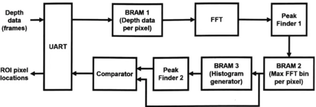
The automatic ROI detection algorithm was implemented on an FPGA. The block diagram is shown in Figure 2-4. For simplicity, the first and final steps of the algorithm (detrending and taking a subset of the resulting pixels) were not implemented. A UART is used for serial communication between the FPGA and computer. BRAMI stores the depth data for 4800 pixels across 192 frames (see Section 2.1.2), so its size is 4800 x 192 = 921600 words, with 12-bit words. The data was augmented with zero padding and passed through a 512-point FFT. Peak finder 1 determines the maximum bin for each pixel and stores them in BRAM2. The peak FFT bin can be in the range of 0 to 255 (since the 512-point FFT is symmetric) which can be stored with 8 bits, so the size of BRAM2 is 4800 words, each containing 8 bits. BRAM3 stores the histogram, which has 256 possible bins, each storing a count of up to 4800, requiring 13 bits. Peak finder 2 determines the peak bin in the histogram. The values
Depth BRAM I Peak
data (Depth data FFT Finder 1
(frames) per pixel)
UART
BRAM 3 BRAM 2
Comparator F (Histogram (Max FFT bin
locations Finder 2 geertr) pr pixl
generator) per pixel)
Figure 2-4: Block diagram of FPGA implementation of automatic ROI detection.
in BRAM2 are compared with the histogram peak. If the peak bins match, a 1 is sent back through the UART to indicate that a pixel should be included in the ROI. Otherwise, a 0 is transmitted.
2.1.2
Frequency Estimation
Previous works have extracted the breathing rate from the average depth signal using two main methods: (1) Fast Fourier Transform (FFT)
[71,
and (2) peak detection[6].
The advantage of the FFT-based approach is that it is able to provide a new breathing rate estimate at every time step (though it requires one window of data to obtain the first estimate). However, disadvantages include low resolution, slow response time (on the order of the window size), and sensitivity to amplitude variations. On the other hand, using peak detection provides faster response and a more accurate representation of the instantaneous breathing rate, but is more sensitive to noise and can only update on the breathing rate on the next peak (resulting in a stepwise output).In our case, the most critical concern is noise, since the camera we use has particularly low resolution (60 x 80). With higher image resolution, more correlated pixels can be averaged together to reduce the noise. The noise makes peak detection unreliable (see Figure 2-5). Therefore, we prefer an FFT-based approach for extracting the breathing rate from the depth data. Peak detection is more suitable for the reference data from the respiratory belt since that signal contains much less noise.
475 E -C 4-I465 0 0 5 10 15 20 Time (s)
Figure 2-5: Erroneous peak detection on noisy data.
FFT Resolution
Typical breathing rates range from 10 to 60 breaths per minute, or 0. 16 to 1 Hz. Thus, a frame rate of 10 Hz will be enough to capture the frequencies of interest.
There is a tradeoff between frequency resolution and response time in the selection of the window size. A longer window will provide higher resolution, but will result in slower response to changes in breathing rate. We use a window size of 192 points (19.2 s at 10 frames per second), which gives a frequency resolution of around 3 breaths per second. To increase resolution, zero-padding to 512 points was used, increasing the resolution to around 1 breath per second.
Frequency interpolation can be used to further increase the resolution. This is done by fitting a quadratic to the three points around the peak, as illustrated in Figure 2-6. If the magnitudes of the three points are a, /, and y, the relative peak location (p) is given by
a -P=2(a - 2 +) and the magnitude at the peak is
Peak Es6Mae
magniude y(p)
I
ii
I
-1 0 p 1 OFT bin
peak bin srae
peak
Figure 2-6: Quadratic interpolation of frequency peak. Figure from [I].
Note that increased resolution does not directly translate to increased accuracy. The accuracy still mainly depends on the quality of the collected data. But with low resolution, the deviation from the true value will always be high.
FPGA Implementation
The frequency estimation portion of the algorithm was also implemented on an FPGA (separate from the ROI detection). It consists of a UART, 512-point FFT, and peak finder. The output is the peak FFT bin. Frequency interpolation is not performed.
2.2
Results
2.2.1
Test Setup
We used the TI OPT8320 ToF camera to capture the depth data and the Neulog res-piration monitor belt (containing a pressure sensor) to provide the reference breathing
Average 512-point depth FFT per frame UART Breathing
rate Peak Finder estimate
Figure 2-7: Block diagram of FPGA implementation of frequency estimation. signal. These were both connected to a computer through USB. We designed a custom
GUI in Python to synchronize the data between the two devices and to perform
real-time analysis (Figure 2-8). The TI Voxel library was used to interface with the
ToF camera, while the serial library was used to interface with the respiratory belt.
The program can analyze the data in real-time, displaying the depth and amplitude
frames, ROI (possibly user-defined or automatically detected), average depth over the
ROI, signal from respiratory belt, FFT of the previous two signals, and the extracted breathing rate from the two signals. It can also save and load captured frames for
further analysis. For the test videos, the subject was asked to sit directly facing the camera, roughly 0.5 to 1 m away, with their chest and abdomen in the field of view of the camera.
2.2.2
ROI Detection
The automatic ROI detection appears to work well, as the selected regions are similar to ones that would be selected manually. In particular, the results show that the breathing signal is strongest around the chest and abdomen, which is consistent with our expectations. Sometimes, one of the two provides a more dominant signal, and
this is reflected in the selected ROI (Figure 2-9). Figure 2-10 shows the different ROI when only a subset of the pixels (the ones with the largest amplitudes) are
File options Camera parameter --control
Depth
r
frame Region-of-interest (ROI) Amplitude frame Average - depth in ROI Reference signal -- FFT Breathing rateFigure 2-8: GUI used for system testing.
selected. Using around 300 pixels for the ROI seems to provide a good balance between including all the relevant pixels, without including too many extraneous pixels (e.g. background, foreground, or other parts of the body that do not contain breathing content). Compared to [71, which selects the ROI by combining regions around a small set of points containing the strongest signal, our method is more flexible and can more accurately detect the entire region over which the signal is present.
.3
'Ii
'U(a) (b) (c)
Figure 2-9: Automatically selected ROI (ROI size = 300 pixels) from various subjects with the breathing signal concentrated in (a) both the chest and abdomen, (b) mainly
the abdomen, and (c) mainly the chest. I I
(a) (b) (c)
Figure 2-10: Automatically selected ROI, with an ROI size of (a) all valid pixels, (b) 300 pixels, and (c) 50 pixels.
2.2.3
Accuracy
The results from running the complete breathing rate extraction algorithm are shown in Figure 2-11. The first case shows a relatively high breathing rate. There is some amplitude variation around t = 20 s, leading to some inaccuracies in the estimated breathing rate. This error is not corrected until the sliding window no longer contains this amplitude glitch. After this (around t = 40 s), the calculated breathing rate tracks the reference fairly closely. The second case shows a more steady amplitude at a lower breathing rate. Here, the calculated and reference breathing rate are well aligned throughout the entire test interval. The calculated breathing rate is generally accurate to within 1 breath per minute, which is around what we would expect with the selected FFT length with zero-padding.
2.2.4
Summary
The ROI detection works well across a range of test subjects, correctly identifying the location of the strongest breathing signal. The final breathing rate extraction faces some difficulty when there are amplitude variations in the breathing signal caused by sudden movements. It works best when the subject is relatively stationary, which would often be the case in sleep and baby monitoring applications.
zU~AJ 1500 0-0 10 20 30 40 50 60 v-.410C 40C
~VWAM~$MM~
0 10 20 30 40 50 60 E 20 :i10 ~0L.
0 10 20 30 40 50 60 Time (s) (a) 200 .e ~~AAAXM U 0 10 20 30 40 50 60 485 480 475 470LJ 0 10 20 30 40 50 6C 15 a10-0 10 20 30 40 50 60 Time (s) (b)Figure 2-11: Sample results of final estimated breathing rate, along with reference signal.
-e
Chapter 3
Efficient Processing Element
Architecture Supporting Compressed
Weights
3.1
Factored Computation
In neural networks, the majority of the computations can be expressed as a series of multiplications and accumulations (MACs), or a dot product between an activation vector and weight vector. This can be written as
N
b= d = aiwi (3.1)
i=1
where b is a scalar output activation, a is the vector of input activations, and W is the vector of weights. Normally, the weights are represented in 16-bit fixed-point, resulting in 216 = 65536 different possible weight values. However, if the weights are restricted
to a small subset of these values (as in the compression schemes presented in [15] and
[16]), the computations can be done more efficiently by grouping all the accumulations
weights afterwards. We call this technique factored computation.
Suppose for a particular layer in the network, we compress the weights to k unique values such that wi E {w 1, ' - ) W
}.
Let Ij = { I wi = wj } be the set of indices ofthe weights corresponding to the compressed weight value we,. The sets {I1, ... , I k}
partition the input activations into k sets, each of which share the same weight coefficient, and therefore can be combined before multiplication. The computation in (3.1) can be rewritten as N b = a iw i=1 k j=1 iEIj k EWej ai (3.2) j=1 (iEIj
Performing the computation as in Equation (3.1) would require N MACs. However, if we factor out the compressed weights as in Equation (3.2), we would only require N + k accumulations and k multiplications. Block diagrams of these two approaches are shown in Figure 3-2. The inner summation in Equation (3.2) corresponds to the accumulations performed in the k accumulators, while the outer summation corresponds to the output combination. When N is much greater than k, the second approach provides a more efficient method for computing the output since the number of multiplications becomes significantly reduced. From a hardware perspective, this improvement in computational efficiency comes at the price of additional storage required to store multiple accumulator values simultaneously. A more detailed energy estimate taking into account additional hardware considerations will be provided in Section 5.2.
Weight wi V wic Look-Up a SEN1 Wi,C EN1 (a) EN, W -,ON Accumulator 1 ENk mmAccumulator k a (b)
Figure 3-1: (a) Typical computation method: multiplication and weight look-up are performed before each accumulation. (b) Alternative computation method: multipli-cation and weight look-up are performed after all accumulations are completed.
3.2
Performing General Fixed-Point Computations
There are several ways to reformulate general fixed-point computations to map onto the same hardware that performs the alternative computation method in Figure 3-1b. The main constraint is that multiplications (if any) should be performed after accumulations. For example, one way is to perform the multiplication in a bit-serial manner in which one bit of the weight is processed at a time [20]. With M-bit weights, we would need M accumulators, each corresponding to one bit of the weight. If the j-th bit of the weight is a 1, then the activation gets added to accumulator j.
Otherwise, the accumulator value is unchanged. It takes M accumulations to process one weight. After all the accumulations are completed, the final output value can be computed by shifting each accumulator by its index (i.e. shift the value stored in accumulator j to the left by
j
bits) and adding them all up. This can be expressed mathematically as: N b aw N M-1 =Z ajZE(wj< )) i=1 (j=0 M-1 N E E(aiwi,j) < j(3.3) j=0 2i==1where wij is the j-th bit of wi. The form of Equation (3.2) and Equation (3.3) are similar, which suggests that the computations can be easily mapped to the same hardware. However, instead of multiplying with a weight value in the outer summation, Equation (3.3) only requires shifts. Another key difference is the total number of accumulations in this approach for general fixed-point computation is M times greater (i.e. it takes M times longer to process each weight).
in representation of wi in the second line of Equation (3.3). To handle signed multiplication, we just need to make a small modification by subtracting the result associated with the signed bit (accumulator M - 1) rather than adding. To see this, note that if wi is signed, the value it represents is
M-2 wi -wi,M_12m-1 +
S
-j j=0 M-2 = - (wi,M-1 < M - 1) + (wij < j) (3.4) j=0Substituting this for wi in Equation (3.1) and simplifying gives
N M-2 /N
b = - (aiwi,M-1) < M - + (N (aiwj) <j (3.5)
i=1j=0 i=1
which is the same as Equation (3.3) except for the negative sign in front of the terms involving the signed bits (wi,M-1). This subtraction can be done at the either the accumulation step (if it is supported) or at the output combination step.
Other reformulations are possible by processing a group of bits of the weight at a time and also by allowing shifts to occur at the input activation side. This changes the number of accumulators required and the total number of accumulations that need to be performed for each weight.
3.3
Mapping to Hardware
3.3.1
General Hardware Structure
The proposed processing element (PE) for performing the alternative computation method, designed in collaboration with Wanyeong Jung [2], is shown in Figure 3-2a. The basic blocks of the design include a central accumulator array, row decoder,
weight and activation buffers, and output combiner. An array structure was chosen to leverage the reuse of input activation and weight data. The fixed cost of fetching this data from memory would be shared amongst the elements in the array. The accumulator array stores all the intermediate accumulated values prior to output combination. Each square in the array represents an accumulator group (Figure 3-2b) consisting of k accumulators, where k is the number of unique weight values for a specific layer. The row decoder selects which rows of the array to enable based on the compressed weight values. The weight and activation buffers provide the values to be broadcast to the array. Weights are shared across a row of accumulator groups, while activations are shared across columns. The output combiner performs the linear combination of the intermediate accumulated values to generate the final output: the values stored in a row of accumulators is read out, multiplied by the corresponding uncompressed weight, and added to the final output accumulator.
3.3.2
Flexibility
Only the output multiplier block needs to be modified in order to support different uncompressed weight bit-widths, floating point weights (possibly useful for training), and other quantization schemes such as quantizing to powers of 2 (replacing multipli-cations by shifts). Another possibility is to support symmetric weights by allowing subtraction in the accumulator array. This would halve the number of accumulators in each accumulator group, while still operating on the same number of uncompressed weights.
El
jiLii
2 03I
I T ITI
Activation buffer ON E (a) wlo EN, I Accumulator 1i .I
II
ENk if
AccumItor
k
I I U mm mm mm1 (b)Figure 3-2: (a) PE structure [2]. (b) Accumulator group.
IN 42 I b. T b. I b. I b.I
Chapter 4
Dataflow in the Proposed
Architecture
4.1
Overview
A neural network involves different types of layers including convolutional,
fully-connected, batch normalization, non-linearity, pooling, and concatenation layers. All these operations must be supported by the hardware in order to evaluate the output of a network. This requires a detailed mapping of these operations onto the hardware. A typical CNN layer has on the order of 108 to 10' operations. This is usually too many to process in parallel in a single PE so determining how to optimally divide these large tasks into smaller subtasks that can be run on multiple PEs or sequentially on the same PE is important for efficient processing. In this section, we will discuss the mapping of several operations onto the hardware, as well as task division strategies.
4.2
Mapping Operations onto the Processing Element
Some of these operations (such as non-linearities) can be processed quite simply in a separate ALU. Other operations (such as channel concatenation) just require some
manipulations in the memory, so they also do not need to be mapped to the PE array. Convolutional and fully-connected layers make up the bulk of the operations required in typical CNNs. Mappings for these will be discussed in more detail below. Separable convolutions made up of pointwise (1 x 1) and depthwise (2-D) convolutions have recently become more widespread (e.g. MobileNet [21]) due to their ability to dramatically reduce the computational complexity of networks and will also be examined.
Compared to a standard implementation, our proposed architecture requires more storage for intermediate output activations (roughly 16 x with 4-bit compressed weights), roughly the same storage for input activations, and less storage for weights (due to the use of compressed weights). Thus, to minimize the data movement, it is best to adopt an output stationary dataflow, where we try to process as many computations corresponding to one output before writing the result to memory. This requires input activations and weights to be read in repeatedly. In the array, each accumulator group will correspond to one output pixel. Afterwards, we will prioritize input activation reuse over weight reuse because input activations will typically have longer bit-widths.
4.2.1 Depthwise Convolutions
Depthwise convolutions are simply 2-D convolutions between one input channel and a 2-D kernel, generating one output channel. They make up one part of separable convolutions. Combined with pointwise convolutions, they approximate general convolutions, while containing fewer parameters and requiring fewer operations.
Mapping
Figure 4-1 shows the detailed mapping of a depthwise convolution involving one input channel (5 x 5) and one filter (3 x 3) to generate one output channel (3 x 3), on a 3 x 4
accumulator array. Each row of the accumulator array stores one row of the output image. One row of input activations and one column of the filter are loaded. The input activations and filter weights are then shifted and accumulation is performed again. This is repeated until all the filter columns are cycled through. After, the next row of the input image is loaded while the filter weights are loaded again starting from the left most column. Note that the maximum number of rows that can be activated is equal to the number rows in the filter. When broadcasting rows nears the top or bottom of the input image, fewer rows of the array may be activated because fewer output rows require these values as part of their final computation. For example, assuming no padding, the first row of the input image is only used to calculate partial sums for the first row of the output image. As subsequent rows of the input image are loaded, different rows of the accumulator array will be activated.
It is also possible to load multiple rows of the output onto one row of the accumulator array, but how the input is loaded will be a little more complicated. Instead of simply shifting the input activations, some special processing needs to occur at the boundary between two rows of the input image. Also, the number of rows that can be activated is limited by the input row that is closest to the edge of the image. This could mean that certain input activations need to be loaded more than once.
Task Division
There is only really one dimension over which depthwise convolutions can be divided, and that is by image patches. This adds some overhead because the edges (i.e. top and bottom) of each image patch cannot be processed with the maximum parallelism allowed by this operation. Having more image patches introduces more edges. Task division will almost never be necessary for depthwise convolutional layers because of their size. All the input activations and weights should fit easily into the PE memory.
Discussion
The benefit of separable convolutions are that they reduce the number of parameters and computations compared to a general convolutional layer, but result in much less parallelism that can be exploited (for depthwise convolutions in particular). The maximum amount of output parallelism is equal to the size of the kernel, which is often of size 3 x 3 = 9. This is not high enough to fully take advantage of the benefits of the alternative computation scheme. However, depthwise convolutions make up a small number of the total computations in a network. Even as part of separable convolutions, the depthwise portion accounts for a small fraction of the computations compared to the pointwise convolutions. Thus, the reduced efficiency for these layers is not critical.
4.2.2 Pointwise (1 x 1) Convolutions
Pointwise convolutions are a special case of general convolutions that essentially perform channel mixing. A group of M input channels get mapped to N output channels by N groups of 1 x 1 x M kernels. Each output channel is a linear combination of the input channels. The weights for the linear combination are provided by each 3-D kernel. The size of the output images are the same as the input images. There is both weight and input activation reuse for pointwise convolutions, allowing us to take full advantage of the weight and activation broadcasting.
Mapping
Figure 4-2 shows the detailed mapping of a pointwise convolution involving 2 input channels and 3 output channels (all of size 4 x 4) onto a 3 x 4 accumulator array. Each row of the array corresponds to one output channel. Even though in the figure, only one row of each output channel is loaded onto one row of the array, multiple rows of the output image can be loaded by flattening the image. For each output channel,
wI
w
blo boo bw, ba2bl, b12b2Ob21 b2
aSj Jjb jg j
We
boo bw boa0 b10 b11 b12
0 20 b21 b22
W02 boo bo, bO2
o b_ b1Lii 0 bt2, b I e
1 al aws-"ED
Wi1 boo bo b62-WOO blo bl1 b12 0 Eb2, b211 b22-IaloIal a11 2boo bo, b"a bw b1 buE
I2 aW 21 1an
*
Figure 4-1: Dataflow for a depthwise (2-D) convolutional layer mapped accumulator array. The array is shown on the left while the portion of the being performed is highlighted on the right.
onto a 3 x 4 computation
the weight associated with the same input channel is loaded. The input activations at the same image positions in different input channels are streamed in, along with the appropriate weights. After looping through all the input channels, either the same image patch in the next group of output channels (if the activations are cached) or the next image patch in the same group of output channels (if the weights are cached) can be processed in the same manner.
Task Division
The task can be potentially divided across several dimensions: input channel, image patch, and output channel. It will be least efficient to divide the task along the input channel dimension (except possibly in the case that the number of input channels is high) since it means it will not be possible to complete all the computations for any output pixel within one PE. Thus, the (energy-consuming) output write and combination step will need to done for multiple times for each output pixel.
Dividing by image patches or across output channels are independent and can be both done if necessary. The total PE memory is what limits the size of each subtask. Assuming each subtask processes an image patch of size Px x Py and a group of
N' output channels, the total memory required is 16 x Px x Py x M bits for the
input activations (assuming 16-bit activations) and 4 x M x N' for the weights. For maximum utilization of the array, the image patch size (PxPy) should be a multiple of the number of columns in the array and the number of output channels processed
(N') should be a multiple of the number of rows in the array.
Discussion
1 x 1 convolutions map quite naturally onto our proposed architecture. They allow us to exploit the weight and input activation broadcasting much more than for depthwise convolutional layers.
b2 b201 b20 2 b203
bOOO bee
bOO2 b0031 AS b 01
bI
ab 0 bmI
b2 1 bm b20 3 b1I
b1 1 b,02 b1, bgj b., b P bPO1 1 a8 ,aimI
a 1 I a3 b210 b21 b212 b213 b11i
bill b,12 b,13 b,1o bI b01 ba
1 0j aINI a
1 2a
13I
b21o b21 1 b212 b21 3 bilo bill b,12 b, 13boilbonl
ben bo1
a1 10 a1 , a 2 a11
Figure 4-2: array.
Dataflow for a 1 x 1 convolutional layer mapped onto a 3 x 4 accumulator W02 wo1 WOO
W12
wi W10 =*E
MM I II
i
wm l I4.2.3
General Convolutions
In a general convolutional layer, M input channels are mapped to N output channels through N groups of M 2-D filters. In a group of M filters, each filter corresponds to an input channel, and the entire group generates a single output channel. Each of the M filters is convolved with the corresponding input channel and the results are added together to obtain the output channel.
Mapping
General convolutions have characteristics of both depthwise and pointwise convolutions, so the dataflow can be made to resemble either. Pointwise convolutions map more naturally onto the array than depthwise convolutions, so it would be preferable to use a similar approach here. This is illustrated in Figure 4-3, which shows the detailed mapping of a general convolution involving 2 input channels (5 x 5), 3 output channels (3 x 3), and 3 groups of 2 filters each (all 3 x 3), onto a 3 x 4 accumulator array. Like in the case of pointwise convolutions, each row stores a different output channel. One weight per filter group is loaded, each at the same location in the filter group. One row from the first input channel is loaded. Weights and input activations are then shifted, like in the case of depthwise convolutions. After cycling through the first row of the filters, the next row is loaded along with the next row of the same input channel. Then, the next input channel is processed with the corresponding filter weights. This
process is repeated to compute the result for the next row in each output channel or for the same row in another group of output channels.
The dataflow above takes advantage of input activation reuse across output channels and also the horizontal reuse (through shifting), but not the vertical reuse. Modifying the dataflow to look more like the depthwise case (i.e. storing multiple rows from the same output channel on different rows of the accumulator array) allows vertical reuse of the input activations to also be incorporated. However, this would result in

![Figure 2-6: Quadratic interpolation of frequency peak. Figure from [I].](https://thumb-eu.123doks.com/thumbv2/123doknet/13923942.449991/27.917.205.732.101.492/figure-quadratic-interpolation-frequency-peak-figure-i.webp)