HAL Id: hal-00654811
https://hal.archives-ouvertes.fr/hal-00654811
Submitted on 23 Dec 2011
HAL is a multi-disciplinary open access archive for the deposit and dissemination of sci-entific research documents, whether they are pub-lished or not. The documents may come from teaching and research institutions in France or abroad, or from public or private research centers.
L’archive ouverte pluridisciplinaire HAL, est destinée au dépôt et à la diffusion de documents scientifiques de niveau recherche, publiés ou non, émanant des établissements d’enseignement et de recherche français ou étrangers, des laboratoires publics ou privés.
Mickaël Fabrègue, Sandra Bringay, Pascal Poncelet, Maguelonne Teisseire,
Béatrice Orsetti
To cite this version:
Mickaël Fabrègue, Sandra Bringay, Pascal Poncelet, Maguelonne Teisseire, Béatrice Orsetti. Mining microarray data to predict the histological grade of a breast cancer. Journal of Biomedical Informatics, Elsevier, 2011, 44 (Suppl 1), pp.S12-S16. �10.1016/j.jbi.2011.03.002�. �hal-00654811�
Mining microarray data to predict the histological grade of a Breast
Cancer
Mickael Fabreguea, Sandra Bringaya,b, Pascal Poncelet,a, Maguelonne Teisseirec, B´eatrice Orsettid aLIRMM UM2 CNRS, Montpellier, France
bMIAp UM3, Montpellier, France cCEMAGREF, Montpellier, France dINSERM U896-UM1-CRLC, Montpellier, France
Abstract
Background: The aim of this study was to develop an original method to extract sets of relevant
molecular biomarkers (gene sequences) that can be used for class prediction and can be included
as prognostic and predictive tools. Materials and Methods: The method is based on sequential
patterns used as features for class prediction. We applied it to classify breast cancer tumors according
to their histological grade. Results: We obtained very good recall and precision for grade 1 and 3
tumors, but, like other authors, our results were less satisfactory for grade 2 tumors. Conclusions:
We demonstrated the interest of sequential patterns for class prediction of microarrays and we now
have the material to use them for prognostic and predictive applications. Keywords:
1. Introduction
Breast cancer is a major public health issue today. According to the breastcancer.org1, with
192,370 new cases in 2009 in the U.S., breast cancer is the most frequently diagnosed malignancy and
the main cause of cancer death in women. One out of eight women will develop breast cancer during
her lifetime. New treatments are continually being developed to target specific types of cancer and to
reduce potentially adverse effects (cardiac dysfunction, premature menopause, etc.). However, despite
early detection and new treatments, up to 50% of the women will develop distant metastases, which
are unfortunately incurable today. The three major challenges associated with breast cancer are: (1)
How to diagnose breast cancer as early as possible through population screening and to identify the
type of tumor detected? (2) How to predict the response of a patient to a given treatment according
to classes of individuals? (3) How to choose the best therapy for a given subject with an accurate
prognosis including her chances of remission, by deducing from the usual course of the disease its
future development and its outcome?
DNA microarrays are powerful tools to draw a genetic portrait of a biological sample (e.g., a tumor
sample) by comparing gene expression in different tissues, cells, and conditions, and providing
infor-mation on the relative levels of expression of thousands of genes among samples. These technologies
carry with them the hope of bringing new insights to cancer biology and improving current tools for
cancer management. Simon and Dobbin [1] describe three ways of using DNA microarrays:
• Class comparison consists in identifying variations (e.g., in the expression of the genes) among
n classes. It can be used to compare normal tissues and tumors [2], and tumors that respond
to therapy and those that do not [3], or to distinguish various subtypes of a tumor [4, 5].
Class comparison enables identification of the critical role of certain genes by establishing the
molecular identity of a class, like a bar code. This code can then be used for class prediction.
• Class discovery consists in discovering new subgroups in a population (e.g., subtypes of a tumor)
based on the molecular profile. For example, Sotiriou et al. [5] describe subtypes of breast cancer.
• Class prediction uses the results of the previous process to assign a new specimen (a new
microarray) to a known class, e.g. to a subtype of a tumor [6]. If the classifier is confident, the
result can be used by medical experts to make clinical decisions (e.g., for population screening)
to predict the effects of a treatment for a patient or for prognoses.
The objective of this study was to develop an original method to extract sets of relevant molecular
biomarkers (gene sequences) that can be used for class prediction and as a prognostic and predictive
tool. Molecular biomarkers are generated from analyses of DNA microarrays and are based on a
particular data mining technique: Sequential pattern discovery. In [7], we described an efficient
algorithm to extract these frequent patterns of correlated genes ordered according to their level of
expression. An example of such a pattern is < (17aagovcadn)(tgzadipup, rettdn) >,80%Gr1, 40%Gr2
meaning that ”For 80% of Grade 1 tumors, and 40% of Grade 2 tumors, the level of expression of gene
17aagovcadn is lower than that of tgzadipup and rettdn, whose levels of expression are very close”.
Sequential patterns have already been used successfully for text categorization. In this paper, we
investigate the relevance of such patterns for tumor classification. The complexity of the data and
the interdisciplinary context make this task extremely challenging.
Our contribution is described in terms of methodology, biological findings and medical implications.
After briefly presenting the state of the art (section 2), we describe the complete methodology in
detail in the material and methods (section 3). We apply this methodology to the study of breast
cancer (section 4). To conclude, we discuss how this methodology can be generalized (section 5)
2. Background
Due to the amount of data available, processing DNA microarrays in a way that makes
biomed-ical sense is still a major issue. Statistbiomed-ical methods and data mining techniques play a key role in
discovering previously unknown knowledge. However, their implementation in this context is difficult
because the number of measurement points (gene expression levels) is much higher than the number of
samples, which results in the well-known problem of the curse of dimensionality, also called the high
feature-to-sample ratio [4]. Moreover, the correlation structure of the expressions is unknown (gene
co-expressions) and the presence of noise is a serious problem. For all these reasons, classification
based on microarray data is quite different from previous classifications and traditional methods are
not successful [8].
Most studies are based on the search for differentially expressed genes, particularly disease-specific
genes. These methods work like a filter and reduce the size of the group of genes in the experiment
to a smaller one, which can be more easily investigated. Most widely used methods use univariate
procedures often combined with adjustment of P-values or a similar concept [9, 10]. SAM [10] or
CyberT [11] are well-known programs based on such techniques. Unlike multivariate approaches such
as ANOVA, these methods do not take into account the multidimensional structure of the data [12].
We could also cite other approaches based on combinations of various artificial intelligence techniques
[13, 7]. However, several authors [14, 9] have compared most of these methods and shown that they
do not necessarily detect the same subset of differentially expressed genes.
Nevertheless, the above-mentioned methods do help rank the genes for the development of
biomark-ers that can be used for class discovery. Differentially expressed genes are features used to discriminate
subgroups of specimens. Many diseases are heterogeneous and characterized by the presence of several
information and responses to therapy and the molecular signatures that characterize subgroups has
greatly facilitated the development of treatments tailored to specific subgroups. To discover the
sub-groups concerned, we focus on the case where the experiments monitor the gene expression of different
tissue samples, and the aim is to find a structure in this collection of unlabeled data to associate with
a category, describing, for example, a subgroup of tumors. Several authors [16, 15, 5] have published
such lists concerning breast cancer.
Once the subgroups are defined, it is possible to associate a new microarray with a class with
class prediction by comparing a new specimen to features describing the subgroups. Several authors
[17, 18, 16, 19] have proposed successful methods but it is still too difficult to use them to improve
breast cancer prognosis or prediction [20]. The pitfalls have been emphasized by many authors
[21, 1], these include the risk of over-fitting due to the high feature-to-sample ratio and the lack
of validation due to the absence of independent datasets or the incorrect use of cross-validation
techniques. Although the number of measured genes is in the thousands, it is assumed that only a
few genes determine the type of a tissue. More recent studies focus on finding such groups of genes.
In this paper, we do not try to find the minimum subsets of genes but look for gene sequences that
we can use as features for the prediction of different classes.
3. Material and Methods
The class prediction system involves two steps: Step 1- Building the classifier: (1) The sequence
preprocessing module transforms the raw data into gene sequences; (2) The feature selection module
extracts sequential patterns, which have a close relationship with a given type of class; Step
2-Evaluation of the classifier: The classification module makes decisions concerning categories of testing
samples and examines whether the classification results are confident or not.
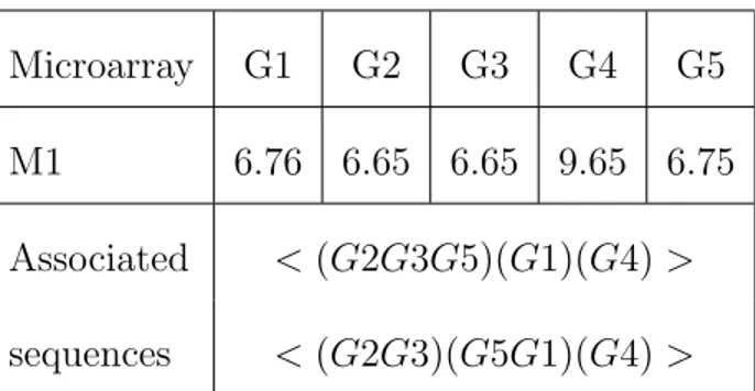
Microarray G1 G2 G3 G4 G5
M1 6.76 6.65 6.65 9.65 6.75
Associated < (G2G3G5)(G1)(G4) >
sequences < (G2G3)(G5G1)(G4) >
Table 1: Gene expressions for microarray M1 and two associated data sequences with a minimal gap of 0.1
3.1. Sequence preprocessing module:
For each microarray, we have a list of genes associated with an expression value (see Table 1).
The aim of this step is to build sequences by ordering the genes according to their value. In classical
database vocabulary, the genes are called items. An itemset iti is a non-ordered group of genes with
similar expression. By considering the gaps between the expression of the genes (see Table 1), G2
and G3 are grouped in the same itemset because they have the same expression, but considering a
minimal gap equal to 0.1, G5 can be either grouped in it1 = (G2G3G5) or in it2 = (G1G5). A
sequence S =< itaitb...itp > is a non-empty and ordered list of p itemsets, i.e. groups of genes ordered
according to their expression. From a microarray, we generate as many sequences as there are possible
itemsets. Table 2 gives associated data sequences with a minimal gap of 0.1.
3.2. Feature selection module:
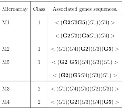
Table 2 gives an example of data used as input in the feature selection module. The aim of this
step is to build sequential patterns [22], in our case frequent sequences of genes, to characterize a
class. A pattern is supported by a microarray if the pattern is included in one or more sequences
associated with a microarray. For example (see Table 2), the pattern P =< (G2)(G5) > is included
in one of the two M 1 data sequences. So, P is supported by the microarray class1. The support of
Microarray Class Associated genes sequences. M1 1 < (G2G3G5)(G1)(G4) > < (G2G3)(G5G1)(G4) > M2 1 < (G1)(G4)(G2)(G3)(G5) > M5 1 < (G2 G5)(G4)(G3)(G1) > < (G2)(G5G4)(G3)(G1) > M3 2 < (G1)(G4)(G5)(G2)(G3)) > M4 2 < (G1)(G2)(G3)(G4)(G5) >
Table 2: Gene sequences for 5 microarrays and 2 classes. The microarrays M1, M2 and M5 are associated with the class 1 and M3 and M4 are associated with the class 2. According to a minimal gap, 2 sequences are associated with the microarray M1 and M5 and 1 sequence is associated with the microarrays M2, M3 and M4.
that support P in that classi. For example, support1(P ) = 3/3 and support2(P ) = 1/2. To obtain
the most frequent patterns, a minimum support is provided and the patterns extracted must have a
support greater this threshold, called the minimum support. For instance, if the minimum support
is equal to 2/3, P is frequent in class1 but not in class2. These definitions were given in a previous
work [4], and an efficient algorithm was developed. In this paper, we have adapted the PrefixSpan
algorithm [23] to take into account n sequences associated with a microarray. [24] have shown that
Prefixspan is pseudo-polynomial. The complexity is O((2N ) ∧ L) where N is the number of items
and L is the maximum length of the initial gene sequences of the microarrays.
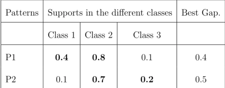
For class prediction, we only look for relevant patterns and not for all patterns. We rank the
patterns to keep only the k best patterns for each class according to a measure based on the support
value. For each pattern, the ranking measure is the difference between their two highest supports.
Patterns Supports in the different classes Best Gap.
Class 1 Class 2 Class 3
P1 0.4 0.8 0.1 0.4
P2 0.1 0.7 0.2 0.5
Table 3: Gaps obtained for two patterns for 3 classes. For each pattern, support has been computed for each class. For a particular, the best gap is equal to the difference between the two highest supports. In this example P2 ”is better” than P1 because P2 has the highest best gap.
P 2, 0.5. Consequently, pattern P 2 has a better rank than pattern P 1. The interest of these patterns
is that they can be used to distinguish classes but they also enable to take into account additional
information with respect to differentially expressed genes, i.e. the order of expression of correlated
gene groups.
3.3. Classification module:
The objective is to assign S =< (G1)(G2G3)(G4)(G5G6)(G7)(G8)(G9)(G10G11) > an unlabelled
sequence to a class (a category of tumor). We compare S to n% of the ranking patterns by class.
Consider the patterns P 1, P 2, P 3 (see Table 4), with P 1, P 3 for class2, and P 2 for class3. When S
contains a pattern, the score of S for the class associated with the pattern is increased by 1. Table 5
gives the score of S for each class. As the highest score is for class2, S is assigned to class2.
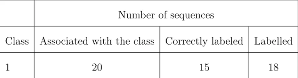
To evaluate the classification, we measure the precision and the recall for each class. Precision
is the number of sequences correctly assigned to a class divided by the total number of sequences
assigned to this class (correctly or not). The recall is the number of sequences correctly assigned to
a class, divided by the number of sequences of real data belonging to this class. Table 6 gives an
Patterns Class 1 Class 2 Class 3
P 1 =< (G1)(G2G3)(G4) > 0.2 0.8 0.1
P 2 =< (G5G6)(G7)(G8) > 0.1 0.0 0.9
P 3 =< (G9)(G10G11) > 0.3 0.7 0.1
Table 4: Distribution of the sequential patterns in 3 classes. As P1 and P3 have the highest support in Class 2, they are associated with Class 2. P2 is associated with Class 3.
Sequence Class 1 Class 2 Class 3
S =< (G1)(G2G3)(G4)(G5G6)(G7)(G8)(G9)(G10G11) > 0 2 1
Table 5: Scores by class associated with sequence S. According to the distribution in Table 4, the sequence S is included in 0 pattern of class 1, in 2 patterns of class 2 and in 1 pattern of class 3.
Number of sequences
Class Associated with the class Correctly labeled Labelled
1 20 15 18
Table 6: Example of results obtained after cross validation. Precision=15/20, Recall=15/18 and F-measure= 2*(15/20*15/18)/(15/20+15/18))
F = 2 ∗ precision ∗ recall
precision + recall (1)
4. Experiments
Datasets and objectives: We examined the following microarray datasets: a dataset provided
by the IRCM which is not public, and datasets available online from Gene Expression Omnibus2
KJX64-KJ125 (GSE2990), TAM (GSE6532), and TBG2 (GSE7390), focusing on a total of 624 human
Affymetrix microarrays HG 133. All these microarrays share 22000 probesets3. To start the study, we
focused on a subset of this list, the 128 genes identified by [5] for breast cancer. Below, we illustrate
the power of classification based on sequential patterns in the case of breast cancer through one
question: how to classify a new microarray according to its histological grade [25, 26]? This grade is
a well-known variable with three values. It is used in clinical studies for its high prognostic potential
in breast cancer. For example, patients with a grade 1 tumor have better survival rates than those
with a grade 3 tumor. The distribution of the microarrays is 162 for grade 1, 274 for 2 and 185 for 3.
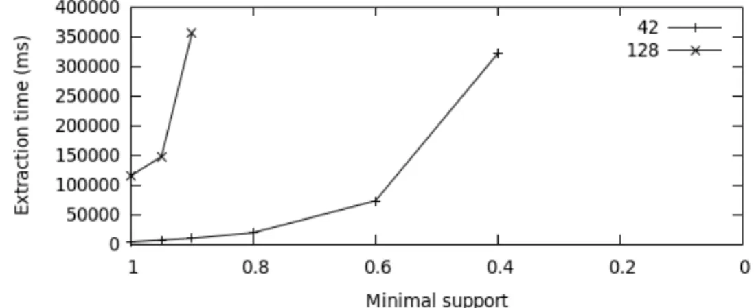
Figure 1: Extraction time vs. minimal support
2http://www.ncbi.nlm.nih.gov/geo/
Extraction of sequential patterns:
The extraction parameters are defined experimentally. As shown in Figure 1, in this type of data,
it is difficult to extract patterns with a minimum support in a reasonable timeframe (we only keep
patterns with a support greater than a given threshold named minimum support). We do not look
for all patterns but only for a subset of patterns enabling efficient classification. For rapid extraction,
we split the gene base into few groups and extract patterns from each. We experimentally vary the
number of genes and the support. We observed that the most accurate approach is to form groups of
42 genes that can be extracted in 350 seconds with a miniuml support of 0.4.
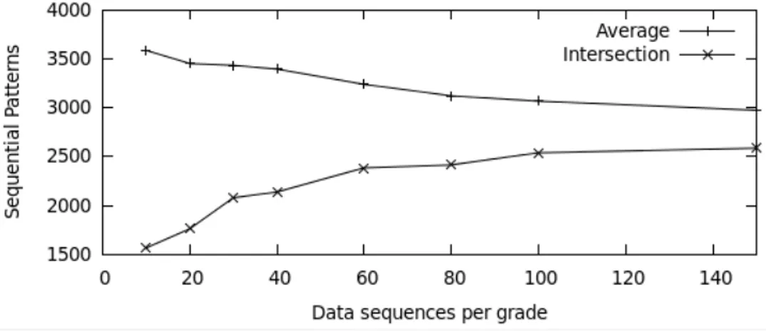
Figure 2: Stability of the generation of the patterns
In Figure 2, we gradually increase the number n of microarrays used for the extraction. For
each n, we randomly select n microarrays per class, extract the patterns m times (m = 20), and
count the number of common patterns. The higher the n, the more extracted patterns are the same.
Experimentally, we fixed n at 80 per grade to get a consistent training set and to keep enough
microarrays to be able to validate the classifier in the validation set.
Classification: We used a cross-validation process to assess how the results of our classifier are
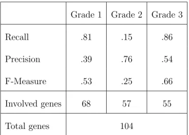
Grade 1 Grade 2 Grade 3 Recall .81 .15 .86 Precision .39 .76 .54 F-Measure .53 .25 .66 Involved genes 68 57 55 Total genes 104
Table 7: Evaluation of the classifier per grade. For a total of 104 genes (68 involved in sequences associated with Class 1, 57 with Class 2 and 55 with Class 3), we obtain various measures of Recall, Precision and F-measure by class.
into complementary subsets, building the classifier on the training set, and validating the analysis on
the validation set. According to the results deduced from Figure 2, we extracted sequential patterns
on 80 specimens (38% of the total base) and validated the classifier on the remaining specimens (62%).
To reduce variability, multiple rounds (50) were performed using different distributions. We used the
100 best sequential patterns for each grade.
Table 7 shows the evaluation of the method for the three grades. The method remains valid for
more than three classes. We obtained optimistic results for grade 1 and 3 (Recall) and bad results
for grade 2. These results are consistent with [5] who found that breast cancers of grades 1 and 3
had distinct gene expression profiles that appear in the patterns, but that grade 2 had heterogeneous
gene expression profiles that are not captured by the patterns. In most cases, the specimens are
wrongly classified in grade 1 or 3 (Precision). The line 4 of Table 7 corresponds to the genes used in
the patterns that describe a grade. The last line gives the union between the genes involved in each
grade. It should be noted that the genes are not the same for each grade. The genes can be ranked
according to their efficiency for class prediction thank to the number of patterns in which they appear
Grade 1 and 3 Grade 1, 2 and 3 Classifier IRCM IRCM and online datasets Online datasets IRCM
R P F R P F R P F R P F Rules (9) 0.954 0.967 0.959 0.922 0.922 0.922 0.924 0.906 0.915 0.715 0.706 0.710 Bayes (8) 0.921 0.932 0.926 0.819 0.826 0.822 0.920 0.918 0.819 0.702 0.716 0.708 Functions (5) 0.955 0.970 0.962 0.902 0.901 0.902 0.917 0.918 0.917 0.760 0.802 0.779 Lazy (4) 0.909 0.939 0.923 0.922 0.931 0.926 0.937 0.943 0.940 0.727 0.721 0.724 Misc (3) 0.934 0.942 0.937 0.937 0.934 0.936 0.932 0.936 0.934 0.736 0.714 0.724 Tree (12) 0.928 0.944 0.936 0.943 0.944 0.944 0.938 0.943 0.940 0.765 0.770 0.767 SP 0.962 0.974 0.968 0.896 0.910 0.903 0.891 0.880 0.885 0.769 0.797 0.782
Table 8: Classifier evaluation. Family of classifiers available in Weka are compared to our method in the last line entitled SP in term of Recal, Precision and F-measure. We vary the number of class (Grade 1 and 3 / Grade 1, 2 and 3) and the datasets (IRCM, IRCM and online datasets and online datasets alone). The highest F-measure scores are in bold in this table.
By considering only grades 1 and 3, and the 3 grades (Table 8), we compared our classifier with
those of Weka software that refer to the data mining community. We calculated the recall, the
precision and the F-measure for each group of classifiers. Considering only grade 1 and 3 or only
grade 3, we obtained the higher F-measure with the IRCM dataset in all cases. The results were least
satisfactory when considering the combination of IRCM and online datasets or online datasets alone.
We can make two assumptions: 1) the online datasets are heterogeneous and it is more difficult to
obtain relevant sequential patterns: the microarrays were obtained from patients undergoing different
treatments, with different types of tumor and many others parameters that affect gene expression.
2) Our classifier is more effective for an imbalanced dataset. Unsatisfactory results were obtained
for grade 2 tumors (table 7) with all the datasets, but optimist results with the IRCM dataset.
From a list of patterns, we can effectively classify tumors into grades. Unlike a list of differentially
expressed genes specific to a class, the patterns can be used to compare different classes and thus
provide answers to different questions concerning prognosis. We can take into account all the DNA
patterns) from a limited set of genes (one hundred). A category could be: a grade 2 tumor, between
2 and 3 cm, treated with hormones, etc. Once a patient is classified in a category, we can use the
information about the future of the patient already assigned to a class to predict her resistance to the
various therapies or to make a prognosis for each choice of therapy.
5. Conclusions and Prospects
In this paper, we focus on the classification of DNA microarrays based on sequential patterns.
Our contribution is two-fold: (i) we have developed a classification technique based on sequential
patterns and not on differentially expressed genes, which is the case of most of the methods cited
in the literature; (ii) we checked it experimentally to verify the interest of these features for the
classification of tumors according to their histological grade. We have shown that the method is
effective at highlighting biological differences between grade 1 and 3 tumors and is better than other
classifiers when the datasets are imbalanced. Like the other methods, the classification is not efficient
for grade 2 tumors. We hope to improve these results by using another form of distribution described
by [5]. We try now to improve the patterns extraction module to manage more genes. We can also
go a step further and use this technique for prediction and prognosis.
6. Conflict of Interest
None declared.
References
[1] Simon RM, Dobbin K. Experimental design of DNA microarray experiments. Biotechniques.
[2] Alon U, Barkai N et al. Broad patterns of gene expression revealed by clustering analysis of tumor
and normal colon tissues probed by oligonucleotide arrays. Natl Acad. Sci. USA.
1999;96:6745-6750.
[3] Rosenwald A, Wright G et al. The use of molecular profiling to predict survival after chemotherapy
for diffuse large-B-cell Lymphoma. N. Eng. J. Med. 2002;346:1937-1947.
[4] Dougherty ER. Small sample issues for microarray-based classification. Comparative and
Func-tional Genomics. 2001;2:28-34.
[5] Sotiriou C, Neo SY et al. Breast cancer classification and prognosis based on gene expression
profiles from a population-based study. Proc. Natl. Acad. Sci. 2003;100(18):10393-10398.
[6] Van de Vijver MJ, He YD et al. A gene-expression signature as a predictor of survival in breast
cancer. N. Eng. J. Med. 2002;347:1999-2009.
[7] Paola S, Bringay S et al. Mining Discriminant Sequential Patterns for Aging Brain. Int. Conf.
AIME. 2009;365-369.
[8] Zupan B, Demsar J et al. Machine Learning for Survival Analysis: A Case Study on Recurrence
of Prostate Cancer. Int. Conf. AIMDM. 1999;346-355.
[9] Dudoit S, Yang YH et al. Statistical methods for identifying differentially expressed genes in
replicated cDNA microarray experiments. Stat. Sinica. 2002;2:111-139.
[10] Tusher VG, Tibshirani R et al. Significance analysis of microarrays applied to the ionizing
radi-ation response. Natl Acad Sci USA. 2001;98:5116-21.
[11] Baldi P, Long AD. A Bayesian framework for the analysis of microarray expression data:
[12] Nueda MJ, Conesa A et al. Discovering gene expression patterns in time course microarray
experiments by ANOVA-SCA. Bioinformatics. 2007;23:1792-800.
[13] Li L, Weinberg CR et al. Gene selection for sample classification based on gene expression
data: study of sensitivity to choice of parameters of the GA/KNN method. Bioinformatics.
2001;17:1131-1142.
[14] Choe SE, Boutros M et al. Preferred analysis methods for Affymetrix GeneChips revealed by a
wholly defined control dataset. Genome Biol. 2005;6:R16.
[15] Sorlie C, Perou M et al. Gene expression patterns breast carcinomas distinguish tumor subclasses
with clinical implications. Natl. Acad. Sci. USA. 2001;98(19).
[16] Peng YH. A novel ensemble machine learning for robust microarray data classification. Computers
in Biology and Medicine. 2006;36:553-573.
[17] Alizadeh AA, Eisen MB et al. Distinct types of diffuse large b-cell lymphoma identified by gene
expression profiling. Nature. 2000;403(6769):503-511.
[18] Brown MP, Grundy WN et al. Knowledge-based analysis of microarray gene expression data by
using support vector machines. Natl Acad. Sci. USA. 2000;97(1):262-267.
[19] Wong TT, Hsu CH. Two-stage classification methods for microarray data. Expert Systems with
Applications. 2008;34:375-383.
[20] Pusztai L. Chips to bedside: incorporation of microarray data into clinical practice. Clin Cancer
Res. 2006;12:7209-14.
[21] Michiels S, Koscielny S et al. Prediction of cancer outcome with microarrays: a multiple random
[22] Agrawal R, Srikant R. Fast algorithms for mining association rules. Int. Conf. on VLDB. 1994,
487-499.
[23] Pei J, Han J et al. PrefixSpan: Mining Sequential Patterns Efficiently by Prefix-Projected Pattern
Growth. Int. Conf. on Data Eng. 2001. 215-224.
[24] Duong, G., Pei, J. Sequence data mining, Springer. August 2007.
[25] Elston CW, Ellis IO. The value of histological grade in breast cancer: experience from a large
study with long-term follow-up. Histopatho.1991;19:403-410.
[26] Scarff RW, Torloni H. Histological typing of breast tumors. International histological classification