HAL Id: hal-01947421
https://hal.umontpellier.fr/hal-01947421
Preprint submitted on 7 Dec 2018
HAL is a multi-disciplinary open access
archive for the deposit and dissemination of sci-entific research documents, whether they are pub-lished or not. The documents may come from teaching and research institutions in France or abroad, or from public or private research centers.
L’archive ouverte pluridisciplinaire HAL, est destinée au dépôt et à la diffusion de documents scientifiques de niveau recherche, publiés ou non, émanant des établissements d’enseignement et de recherche français ou étrangers, des laboratoires publics ou privés.
Inventory credit as a commitment device to save grain
until the hunger season
Tristan Le Cotty, Elodie Maitre d’Hotel, Raphaël Soubeyran, Julie Subervie
To cite this version:
Tristan Le Cotty, Elodie Maitre d’Hotel, Raphaël Soubeyran, Julie Subervie. Inventory credit as a commitment device to save grain until the hunger season. 2018. �hal-01947421�
I
nvent
or
y
c
r
edi
t
as
a
c
ommi
t
ment
devi
c
e
t
o
s
ave
gr
ai
n
unt
i
l
t
he
hunger
s
eas
on
T
r
i
s
t
an
L
e
C
ot
t
y
El
odi
e
Mai
t
r
e
d’
Hot
e
l
Raphaë
l
Soube
yr
an
&
J
ul
i
e
Sube
r
v
i
e
&
J
ul
i
e
Sube
r
v
i
e
Inventory Credit as a Commitment Device
to Save Grain until the Hunger Season
T. Le Cotty* E. Maître d’Hôtel† R. Soubeyran‡ J. Subervie§
Abstract
In January 2013, we collected data from 653 farmers in Burkina Faso, who were asked hypothet-ical questions about risk aversion and time discounting. Ten months later, these farmers were offered the opportunity to participate in an inventory credit system, also called warrantage, in which they receive a loan in exchange for storing a portion of their harvest as a physical guar-antee in one of the newly-built warehouses of the program. We found that farmers who exhibit stronger hyperbolic preferences are significantly more likely to participate in the warrantage sys-tem than other, otherwise similar, farmers. We interpret this result as evidence that farmers use warrantage as a means to commit to saving a portion of their crop until the lean season, which may improve their capacity to ensure the food security of their household.
Key Words: Commitment Savings, Inventory Credit, Hyperbolic Discounting. JEL: D14, O12.
*CIRAD, UMR CIRED.
†CIRAD, UMR MOISA.
‡CEE-M, INRA, CNRS, SupAgro Montpellier, Univ. Montpellier, Montpellier, France.
§CEE-M, INRA, CNRS, SupAgro Montpellier, Univ. Montpellier, Montpellier, France. Corresponding author. Email:
[email protected]; Campus INRA-SupAgro, 2 place Pierre Viala, batiment 26, 34060 Montpellier Cedex 1, France. Phone: + 33(0)499 613 131. Fax: + 33(0)467 545 805.
1 Introduction
In developing countries, banks and financial institutions generally shy away from lending to the agri-cultural sector because farmers are highly exposed to production risk and often lack collateral.1There is an abundant literature showing that credit constraints may exacerbate the negative effects of intra-annual grain price volatility, forcing farmers to sell their grain at a low price during the post-harvest season,2 and it has often been argued that providing credit access to poor farmers may help them smooth consumption.3 In this context, inventory credit, also called warrantage, has emerged as a potential solution to this problem.
With warrantage, banks typically offer farmers an advance amounting to 80 percent of the market value of the amount of grain that they elect to secure in a certified warehouse over a six-month period. This is likely to improve farmers’ food security in many ways. First, farmers who have access to credit may be more likely to engage in other income-generating activities, aiming not only to repay the loan but also to better cope with the lean season. Second, farmers who are able to repay the loan and get their collateral back can benefit from a possible increase in grain price. Third, farmers who store their crops as collateral until the time of loan repayment escape the prevalent social pressure to share their harvest with kin and neighbours.4 Last but not least, these farmers circumvent the temptation to sell their grain in order to purchase goods of no long-term value, thereby enabling them to mitigate self-discipline problems that could otherwise limit their ability to save grain.
Warrantage is not yet widespread in Africa. It emerged in Niger in the 2000’s (Coulter and On-umah, 2002) and has been developing in Burkina Faso since 2005.5 A precondition for a warrantage system to emerge is that banks must be confident that the stored product will be available should they need to withdraw it. From a market demand perspective, farmers who are willing to store a portion of their harvest for a period of six months must also be confident that their collateral will be returned once they repay the loan. Thus, each stakeholder in the system relies on the existence of a reliable network of certified warehouses.
1See among others Bester (1987) and Hoff and Stiglitz (1990).
2See Stephens and Barrett (2011); Kazianga and Udry (2006); Dillon (2016); Casaburi and Willis (2016).
3See Burke, Bergquist, and Miguel (2018); Basu and Wong (2015); Fink, Jack, and Masiye (2014).
4Several recent studies indeed suggest that individuals living in poor communities often feel obligated to support rela-tives and neighbours (Platteau, 2000; Barr and Genicot, 2008; di Falco and Bulte, 2011) and that those who anticipate that their income will be “taxed” by neighbours may choose to spend their wealth quickly (Goldberg, 2017) or to hide part of it (Jakiela and Ozier, 2016) in order to escape solicitations. Baland, Guirkinger, and Mali (2011) also suggest that excess borrowing is a strategy used by some individuals in order to signal to their peers that they are cash constrained and cannot respond to their demands.
5Warrantage shares some features with the warehouse receipt systems (WRS) that exist in Ghana, Tanzania, and
Zam-bia, but WRS cannot be considered commitment devices because farmers who own a receipt are able to sell their grains whenever they wish (Coulter, 2009).
We implemented a warrantage system in Burkina Faso and investigated the possible link between farmers’ risk and time preferences and participation in the system. This project was called the Farm Risk Management for Africa (FARMAF) project. We partnered with the Reseau des Caisses Populaires du Burkina Faso, a rural bank operating in Burkina Faso, and the Confédération Paysanne du Faso (CPF), a nation-wide organization of farmers, to implement a warrantage system in the western re-gion of Burkina Faso. In January 2013, a series of hypothetical choice experiments were implemented in the field to elicit measures of discounting and risk aversion for a random sample of 653 farmers spread across seven villages. In 2013, each of the villages was provided a warehouse. In November 2013, each farmer living in these villages was offered credit in exchange for storing a portion of their harvest as collateral in one of these warehouses, with no opportunity to access the stored grain for a period of six months. The warrantage system continued to function in subsequent years.
We collected data on farmers’ participation in the system in 2013 and again in 2015. We found that farmers electing to engage in warrantage stored a quite large portion of harvested crops - around 30 percent. We moreover found that a significant proportion of participants chose to store without taking out a loan, a behavior that cannot be explained by the liquidity constraint. One of the main contribution of this article is to offer a new rationale for the success of warrantage schemes, based on the demand for commitment.
In this article, we develop a theoretical model in which the farmer is sophisticated with respect to present bias and makes decisions about how to allocate his harvest for various uses. In this model, participation in warrantage provides the farmer with a means to constrain his futures selves. The model predicts that participants in warrantage are likely to fall into three categories - those who stored grain and borrowed the maximum amount allowed for a loan, those who stored grain and borrowed less than the maximum amount allowed for a loan, and those who stored grain without taking a loan -something that we actually observe in our data. The model moreover predicts a positive relationship between time-inconsistency and participation into the scheme.
We then match measures of farmers’ risk aversion and time preferences with observed adoption of warrantage. We capture this relationship in a regression which includes a range of observable in-dividual characteristics and village-year dummies. In line with the main prediction of the theoretical model, we find that farmers who exhibited hyperbolic preferences were significantly more likely to engage in the system. We interpret this result as evidence that time-inconsistent farmers use inven-tory credit as a means to commit to saving a portion of their crop until the hunger season. This result suggests that inventory credit is likely to provide support for people who wish to protect their harvest
from their own, possibly short-sighted, impulses. While we cannot entirely rule out the possibility that this result arises due to an unobserved factor affecting both experimental measures of time and risk preferences as well as warrantage adoption (see Section 7 for a discussion of alternative explana-tions), it is worth noting that our findings are consistent with recent studies, suggesting that present-biased people may be particularly willing to engage in commitment devices in order to mitigate the anticipated impatience of their future selves.
Many theoretical models, such as the quasi-hyperbolic discounting model of Laibson (1997) or the temptation and self-control theory proposed by Gul and Pesendorfer (2001), imply a demand for commitment (see Bryan, Karlan and Nelson 2010 for a review of the literature).6These models predict that individuals who exhibit more impatience for near-term trade-offs than for future trade-offs, and are sophisticated enough to realize this, will engage in commitment devices in order to increase their welfare (O’Donoghue and Rabin, 1999). For example, although present-biased individuals may pre-fer today to be patient enough in the future to save the harvest that they store on site, when the time comes they may nonetheless fail to do so when tempted to use their crop for immediate consump-tion. The point is that individuals who realize that they may revisit their choice in the future may seek for a way to “tie their hands” to prevent this from happening. Institutions can help solve self-control problems by providing such a commitment mechanism (Mullainathan, 2005; Bauer, Chytilova, and Morduch, 2012).7In this paper we argue that, for developing countries like Burkina Faso in which for-mal commitment savings mechanisms are lacking, warrantage is likely to provide an effective device in this regard.
Some recent empirical studies have already established a link between hyperbolic preferences and decisions to engage in a commitment device (see Frederick, Loewenstein, and O’Donoghue (2002) for a review to the early 2000s and Sprenger (2015) for more recent papers). It is however dif-ficult to find examples of pure commitment devices provided by the market in developing countries. Participation in a rotating savings and credit association (ROSCA) can be explained by a preference for commitment, since joining a ROSCA makes defaulting very difficult unless one is prepared to bear the associated costs, which can be significant (Aliber, 2001; Anderson and Baland, 2002; Gugerty, 2007; Ambec and Treich, 2007; Basu, 2011). In practice, however, it remains difficult to determine whether people use the ROSCA because they perceive it as a commitment savings device or for other
6Several papers have studied the theoretical properties of hyperbolic discounting (Phelps and Pollak, 1968; Laibson,
1997). Other approaches to model problems of temptation and self-control include Gul and Pesendorfer (2001), Fudenberg and Levine (2006) and Banerjee and Mullainathan (2010).
7Bernheim, Ray, and Yeltekin (2015) theoretically show that some external commitment devices can undermine the
reasons. Evidence supportive of the idea that some people use savings devices for their commitment value would establish an empirical link between the use of a commitment device and the hyperbolic nature of the preferences of its users. Two seminal empirical studies do provide this type of evidence. In a study run in the Philippines, Ashraf, Karlan, and Yin (2006) showed that women who exhib-ited hyperbolic preferences were significantly more likely to open a commitment savings product. In South India, Bauer, Chytilova, and Morduch (2012) found that women who exhibited present-biased preferences were more likely to borrow from a self-help group than from a bank or a moneylender, interpreting this result as evidence that these women use self-help groups as a means to commit themselves to save money each week.8
Our study builds on and extends this literature by providing the first field evidence that links time inconsistency to the decision to engage in a warrantage system, a promising development tool that is emerging in African countries. We show that there is heterogeneity in demand for a storage com-mitment device and that time-inconsistency can explain some of this heterogeneity. Our study thus provides new evidence regarding the relationship between time preferences, credit access, and stor-age choices among Burkinabe farmers, and presumably among farmers in sub-Saharan Africa more generally.
The article proceeds as follows. Section 2 describes the main features of the warrantage system that we implemented in Burkina Faso. Section 3 describes a theoretical model of a sophisticated hy-perbolic farmer’s decision to allocate the harvest between warrantage and alternative uses. Section 4 describes the surveys and Section 5 focuses on hypothetical risk and time preference data. Section 6 discusses how experimental choices correlate with observed adoption of warrantage. Section 7 pro-vides alternative explanations for the apparent link between time-inconsistency and participation in warrantage. In particular, we discuss to what extent our findings may arise due to an unobserved credit constraint or social taxes. Section 8 concludes.
2 Context and FARMAF project
As part of the FARMAF project, we implemented a warrantage system in two administrative districts of Burkina Faso, the Tuy and Mouhoun provinces, in the western region of the country (Figure 1). The
8More recently, Giné et al. (2018) implemented artefactual field experiments in Malawi and showed that the revisions
of money allocations toward the present are positively associated with measures of present-bias. In a developed-country context, Meier and Sprenger (2010) elicited individual time preferences using incentivized choice experiments in laboratory and showed that present-biased individuals are more likely to have credit card debt.
FARMAF project is one of the first programs aiming to develop warrantage in the country.9 Except for the initial cost of building the warehouse and the initial organizational costs, 95 percent of which were covered by the FARMAF project and 5 percent by farmers, the system runs without material or financial assistance. Furthermore the warrantage system seems viable, as it has been implemented each year since 2013.
The warehouses were built in the villages so that farmers can bring their bags themselves with bicycles, motorcycles or donkey pulled carts. The warehouses have a storage capacity of up to 80 tons, which means that 50 households can each deposit 16 bags of 100 kg. In November 2015, i.e. after three seasons of warrantage, 85 percent of the storage capacity was reached. The warehouses are secured with two locks. The key to one of these locks belongs to the rural bank, and the other key belongs to the local farmers’ organization. As a result of this dual-lock system, neither party can open the warehouse in the absence of the other.
The warrantage system was designed to correspond to the agricultural calendar (Figure 2). In the warrantage system as we implemented it, farmers are allowed to store cereals, sesame, and peanuts. Farmers store mainly maize, followed by sorghum and millet, which are characterized by very similar price patterns.10 In Burkina Faso, land preparation and sowing for maize, sorghum and millet typ-ically begin in June, and the crops grow during July and August, maturing between September and October.11 Farmers who participate in the warrantage system receive a loan in November, which is often used to pay seasonal employees for cotton harvesting. Farmers who are able to repay the loan get their collateral back in May, at the lean season, when the price of grain is usually high.
Every year since 2013, farmers were solicited to deposit a portion of their harvest in one of these warehouses in exchange for a 6-month loan. The rural bank does not lend more than 80 percent of the value of the inventory at the time of the loan. Should borrowers default, this protects the rural bank even if the price of grain decreases by 20 percent, which is very unlikely to occur. The monthly interest rate charged by the bank is around 1 percent. The interest rate, as well as the value of the collateral, are determined by the rural bank.12 Farmers were also charged the cost of storage, which amounted
9Previous programs include the warrantage program of the NGO SOS Sahel, which was carried out in eight provinces of
Burkina Faso (Bam, Gnagna, Ioba, Loroum, Mouhoun, Namentenga, Nayala, and Sanmatenga) and the warrantage program of the NGO Comunità Impegno Servizio Volontariato (CISV), which was carried out in the provinces of Tuy and Ioba.
10Farmers may also store beans (niébé), but since the pre-storage drying process is much easier for grains than for beans, farmers tend not to store beans. Another reason why farmers store mainly maize is that maize yields are higher (maize responds better to fertilizer). Sorghum and millet are very much appreciated for self-consumption and traditional usages including making dolo (a kind of traditional beer), whereas maize is not only consumed but is also a cash crop. Cotton, the main cash crop, is not a possible candidate for warrantage, notably because a parastatal board controls the entire cotton sector.
11The length of the cropping cycle is around 100 days for maize and 120 days for millet and sorghum.
to 100 CFA for each 100 kg bag of grain per month. This storage fee is based on information regarding previous warrantage programs that have been implemented in Burkina Faso and Niger. It includes the warehouse maintenance and the transaction costs incurred to deal with credit institutions (phone calls and travel from village to bank agencies). The borrower’s name is written on each bag of grain that is deposited so that each farmer will be able to identify his deposit later. Farmers also have the opportunity to store grain without taking out a loan. When the loan matures, i.e. in May, the bank demands repayment of the amount borrowed plus interest before authorizing the restitution of a farmer’s collateral. If the farmer is not able to reimburse the loan and interests, the collateral is sold. In practice, the farmer must find a buyer and meet him at the warehouse on the repayment date. In this case, the farmer reimburses the bank and keeps what remains. If the farmer is unable to find a buyer on the repayment date, he is subject to a penalty: 10 percent of the total debt per day late. If the farmer defaults, the bank keeps the collateral. We do not have data on the proportion of farmers who had to sell their collateral in order to repay their loan. However, we do know that no farmer received penalties between 2013 and 2015.
Farmers must make a tradeoff between the benefits of participating in the warrantage system (such as access to credit and to a commitment device) and its direct and indirect costs (the opportu-nity cost of the collateral deposit, the obligation to pay storage costs at the time of deposit, the risk of not being able to reimburse the loan, the possible lack of understanding of how the system func-tions, the possible lack of trust, etc.). In this system, the total cost of credit can easily be offset by the rising value of the collateral, which was around 40 percent on average over the last decade according to price surveys made by the Afrique Verte association on local markets.13
However, the warrantage system may not be the cheapest alternative for immediate liquidity when the increase in grain prices is small. Indeed, warrantage is profitable only when the increase in the price of grain is sufficiently large compared to the interest rate. For instance, consider a house-hold that owns some grain with a value of 10,000F (post-harvest) and requires 8,000F for immediate consumption. With warrantage, it must store 10,000F as collateral in order to obtain a loan of 8,000F and will be required to reimburse about 8,500F after six months. If the price of grain does not increase over this time period, it will end up with 1,500F (10, 000 −8,500). Without warrantage, it can sell grain to obtain 8,000F immediately and store 2,000F at home, ending up with 2,000F six months later (con-tinuing to consider the case in which the price of grain does not increase). In this case, selling on the
Bouéré, and 1.2 percent in Bladi, Biforo, and Gombélédougou. The mean value of a 100 kg bag of maize or sorghum as collateral was 10,000 CFA.
market to get cash immediately is obviously more profitable than participating in an inventory credit system.
3 Theoretical framework
In this section, we develop a theoretical model in which the farmer is sophisticated with respect to present bias and makes decisions about how to allocate his harvest for various uses. As we shall see, in this model, participation in warrantage provides the farmer with a means to constrain his futures selves.
3.1 Model
We consider three periods in this model for two reasons. First, hyperbolic discounting comes into play when there are more than two periods. Second, in the context of our study, farmers rarely end up with a surplus of grain at the end of the year.14 As a result, it is reasonable to model decisions regard-ing post-harvest investments over a crop year. The first period is the post-harvest season (November), when the farmer must decide whether or not to participate in the warrantage system. The interme-diate period extends from December to April, when the farmer is not able to access any stored grain as collateral. The final period is the lean season (starting in May), when the farmer is required to reimburse the amount borrowed as well as interest before getting his collateral back.
The available harvest is a quantity of grain, denoted H and expressed in kilograms, which can be consumed by the family, stored on the farm in a traditional granary, sold at the market to purchase other goods, or stored in a warehouse as collateral. Let pt be the price of grain at time t and qt the quantity of grain consumed at time t .
In periods 2 and 3, the (indirect) utility of the household is a constant relative risk aversion (CRRA) utility function U (ct) =(ct)
1−r
1−r where 0 < r < 1 is the risk aversion parameter and ct is the value of the
grain (expressed in CFA francs) that is consumed at time t . We assume, for the sake of simplicity, that there is no utility stream in period 1. The farmer’s expected utility at time t = 3 is denoted EU (c3).
The farmer’s discounted expected utility at time t = 2 is:
EU2= EU (c2) +
1 1 + δ1
EU (c3), (1)
14See Bernheim, Ray, and Yeltekin (2015) or Harris and Laibson (2001) for infinite horizon models that focus on the con-sumption decision problem of a budget constrained individual with (quasi-) hyperbolic time preferences. Although we could have extended one of these models to include the specific features of warrantage, it would have led to a rather un-tractable model.
whereδ1is the discount rate of the second-period self, applied to the utility stream that he receives
period 3. The farmer’s expected utility at time t = 1 is:
EU1= 1 1 + δ1 EU (c2) + 1 1 + δ2 EU (c3), (2)
whereδ1(resp. δ2) is the discount rate of the first-period self, applied to the utility stream that he
receives over period 2 (resp. period 3).
In this model, hyperbolic discounting arises from the fact that 1+δ1
2 does not necessarily equal
³
1 1+δ1
´2
. Let us write the hyperbolic discounting parameter, denoted h, as a ratio of the discount factors: h = − ³ 1 1+δ1 ´2 1 1+δ2
with h ≥ −1. If h = −1, the farmer has standard exponential time preferences, and
1 1+δ2 = ³ 1 1+δ1 ´2
. If h > −1, the farmer has (present-biased) hyperbolic preferences, and1+δ1
2 < ³ 1 1+δ1 ´2 . Notice that this definition is quite general. In the specific case of quasi-hyperbolic preferences (also called theβδ model), we have1+δ1
1 = β 1+δ, 1 1+δ2 = β (1+δ)2 and then h = −β.
At time t = 1, the farmer decides whether or not to participate in the warrantage system. If he opts to participate, he chooses the quantity of grain, denoted w , that is stored in the warehouse as collateral, and the loan rate, denotedθ, with 0 ≤ θ ≤ 0.8. Notice that the value of the loan is then p1θw. In order to be able get his grain back at time t = 3, the farmer must reimburse the principal
amount of the loan as well as the interest (1 + i )p1θw, where i is the interest rate.
In order to take into account the difference between returns to warrantage and returns to alter-native investments (whether on-farm storage or investment in a small business), we assume that the return to the grain stored in the warehouse as collateral equals 1 − σ times the return to the grain that is neither stored in the warehouse nor consumed, whereσ refers to the costs of warrantage and 0 < σ < 1.
In order to keep the model as simple as possible, we assume that the price of grain is low in the first two periods, i.e. p1= p2= p. On the contrary, we assume that the farmer is uncertain about the
price of grain in the last period. The price of grain thus increases in period 3 up to p with probability π > 0 and remains low with probability 1 − π > 0. Let us denote ∆ as the maximum percent increase in the price of grain, i.e.∆ =p−pp .
At time t = 1, the farmer chooses w and θ such that his current period discounted utility (EU1)
is maximised and such that the first-period budget constraint H − (1 − θ)w ≥ 0 holds and 0 ≤ θ ≤ 0.8. At time t = 2, the farmer chooses the consumption level c2that maximizes his period 2 discounted
utility, with:
c2= pq2 (3)
and he faces a budget constraint that is affected by the quantity of grain stored in the warehouse at time t = 1:
H − (1 − θ)w − q2≥ 0, (4)
where the impact of committing to warrantage is clear, as w reduces the amount of grain available for second-period consumption.
At time t = 3, the household consumes all that remains of its grain:
c3= p3¡H − (1 − θ)w − q2¢ + p3(1 − σ)w − p(1 + i )θw, (5)
where p3¡H − (1 − θ)w − q2¢ is the value of savings at home, p3(1−σ)w is the value of the grain stored
in the warehouse, and −(1 + i )pθw is the reimbursement of the loan and the interest. The price of grain in period 3 equals p with probabilityπ and p with probability 1 − π.
3.2 Optimal warehouse storage
We solve the game played by the farmer and his future selves (and characterize the sub-game perfect Nash equilibrium) through backward induction. We focus on the case where the maximum return to grain stored in the warehouse is larger than the reimbursement of the loan,15i.e. (1 −σ)(1+∆) > 1+i . For the sake of simplicity, we moreover focus on the cases where inequality (4) is binding, which oc-curs when h is higher than a certain threshold.16 Proofs are relegated to Appendix B.1. We first look at the optimal warehouse storage and find the following result:
Proposition 1 [optimal warehouse storage]: The optimal share of grain that the farmer decides to
store in the warehouse is: w∗ H = " 1 − θ∗+ · −h(1 + δ1) π[(1 + ∆)(1 − σ) − (1 + i)θ∗]1−r+ (1 − π) [1 − σ − (1 + i )θ∗]1−r ¸1r#−1 ,
whereθ∗is the optimal loan rate.
15Even in the event of a small increase in grain prices, the condition still holds for very high (thus unlikely) values ofσ. 16Establishing a full characterization of the optimal choice of the farmer for all possible values of h would be tedious because the optimization problem is not concave. This would require to compare the expected utility for the solution found in Proposition 1 to the solutions of the problem in the case where the inequality is not binding. In this case, however, several local extrema exist. For the ease of presentation, we do not provide these results.
This proposition leads to clear-cut predictions regarding the effects of time preferences on the opti-mal quantity of grain w∗that is stored as collateral. In particular we have:
Main Prediction [hyperbolic & optimal warehouse storage]: The optimal quantity of grain w∗ in-creases with the hyperbolic preference parameter h.
This result arises because a farmer with sophisticated hyperbolic time preferences has the means to constrain his second-period self through warrantage. In other words, the first-period self can choose a quantity of grain w such that the optimal second-period consumption level is fully determined by the second-period budget constraint (inequality 4 is binding).
This proposition also leads to the prediction that the optimal quantity of grain w∗decreases with the impatience parameterδ1. In contrast, the effect of the risk aversion parameter on the optimal
quantity of grain w∗remains ambiguous, since it appears to play in various ways in the characteriza-tion of the optimal storage.17
3.3 Typology of participants
We then characterize the optimal loan rate, which allows us to highlight a typology of participants in the warrantage scheme. We get the following result:
Proposition 2 [typology]: The optimal loan rateθ∗= l∗/w∗is such that:
• Case 1: The farmer borrows the maximum amount allowed for a loan if her level of risk aversion is sufficiently low, i.e.θ∗= 0.8 if r < r ,
• Case 2: The farmer borrows less than the maximum amount allowed for a loan if her level of risk aversion is intermediate, i.e. 0 < θ∗< 0.8 if r ≤ r ≤ r . Moreover, we have:
θ∗ =1 − σ 1 + i hπ[(1+∆)(1−σ)−(1+i)] (1−π)(σ+i ) i1r − (1 + ∆) hπ[(1+∆)(1−σ)−(1+i)] (1−π)(σ+i ) i1r − 1 , (6)
• Case 3: The farmer does not take a loan if she is sufficiently risk averse, i.e.θ∗= 0 if r > r .
where r =Ln £ π 1−π (1+∆)(1−σ)−(1+i ) σ+i ¤ Ln[1+∆] and r = Lnh1−ππ [(1+∆)(1−σ)−(1+i )] (σ+i) i Lnh(1+∆)(1−σ)−0.8(1+i )1−σ−0.8(1+i ) i .
17This is due to the fact that the risk aversion parameter in CRRA utility functions captures both risk aversion and in-tertemporal elasticity of substitution. It thus also plays a role in smoothing consumption over time.
This proposition reveals a typology of participants in the warrantage scheme. Participants can be divided into three groups, namely, those who store grain and borrow the maximum loan amount allowed, those who store grain and borrow less than the maximum amount allowed, and those who store grain without taking out a loan. This last group is of special interest for our study, since it brings together participants who are exclusively seeking a commitment feature in the proposed scheme, i.e. those farmers who have both sufficiently hyperbolic time preferences and are highly risk averse.
To better understand the characteristics of farmers who store grain but do not take out a loan, we examine the optimal loan rateθ∗ in a model where the farmer has consistent time preferences. In such a model, inequality (4) may not be binding (contrary to the model with hyperbolic time prefer-ences). For this reason, the solution differs from Proposition 1. Proofs are relegated to Appendix B.2. One important result arises from a comparison of the two models: whereas a time-consistent farmer will never choose to store grain in the warehouse without taking a loan, hyperbolic farmers will do so as long as they are sufficiently risk averse (i.e. r > r ), as stated in Propositions 1 and 2.
Proposition 2 moreover leads to the (standard) prediction that the optimal loan rate decreases with the risk aversion parameter.18In contrast, the loan rateθ∗is, perhaps surprisingly, independent of time preferences. The reason for this is that borrowing is not an intertemporal choice as such in our model. Although borrowing means having more cash in hand today and assuming the burden of loan repayment in the future, it does not create any imbalance in the consumption path because the farmer has the means by which to smooth his consumption. He can for example, store grain at home (which will increase his wealth in the second period) or in the warehouse (which will increase his wealth in the third period).
In sum, this theoretical model highlights two important qualitative results regarding our under-standing of farmers’ decisions about whether or not to participate in a warrantage program. First, participants are likely to fall into three categories, defined according to the model parameters (π, ∆, σ, and i). In particular, we find that the group of risk averse farmers who store grain in the warehouse but do not take out a loan is comprised only of farmers with hyperbolic time preferences. Second, time preferences are likely to determine the optimal quantity of grain w∗that is stored as collateral. In particular, we find that the optimal quantity of grain w∗increases with the hyperbolic discounting 18We do not test this prediction using our data because it is a very standard result in the literature. Moreover, the relation-ship between the loan rate and the degree of risk aversion cannot be estimated using a simple reduced form model. This is because, in regressing loan rates on risk aversion for farmers who chose to store grain in the warehouse, we are unable to observe the relationship for the sample as a whole. Here, we confront the standard problem of sample selection (Heckman, 1979).
parameter h. In what follows, we show to what extent our data are in line with these predictions.
4 Survey Data
Our main analysis is based on three surveys: a baseline survey run in January 2013 on a sample of 653 households living in the villages where the warehouses were later built, and two follow-up sur-veys, which were carried out among the subgroup of farmers who participated in the warrantage system in 2013 (the first year of the project) and those who participated in 2015 (the third year of the project).
4.1 Survey Procedure
All data were collected in cooperation with the CPF in 7 villages where the number of CPF members is known to be large. In these villages, we interviewed all CPF members, as well as a number of non-CPF members. For the baseline survey, we stratified the sample such that non-CPF members represented two-thirds of the total number of surveyed farmers. An average of 90 households were interviewed in each village. Twenty investigators and two supervisors were recruited for the data collection. Surveys and experiments were conducted in the Dioula language. The enumerators interviewed the heads of households, who were defined as the person responsible for making the farming decisions of the household.
Of the 653 farmers surveyed in January 2013, 103 (16 percent) accepted the offer to participate in the warrantage system in November 2013. Data on individual loan amounts and quantities stored were collected at the time of their deposits. These 103 farmers were also asked about the total quantity of crops harvested before warrantage.
We returned to the field at the end of 2015, at the end of the third round of the project. Of the seven villages enrolled in the program in 2013, one village had decided to leave the program and not to participate in the 2015 follow-up survey. As a result, we were unable to determine the total number of participants in this village in 2015. Of the farmers surveyed in January 2013 in the 6 other villages, 167 (33 percent) had chosen to participate in the warrantage system in 2015. From these participants we collected another round of data on crop harvest, quantities stored, and loan amounts.
4.2 Sample Characteristics
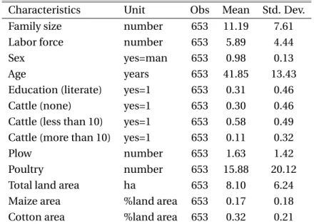
Table 1 reports mean values for various farmer characteristics collected during the baseline survey. On average, the surveyed households are comprised of 11 members, 6 of whom are employed in farming activities. In almost all cases (98 percent), the household is headed by a man of an average age of 42 years, who reports having received a formal education in 31 percent of cases. In the Tuy and Mouhoun provinces, the main crops are cotton, maize, sorghum, millet, and sesame. On average, the surveyed households own 8 hectares of land. They devote about 17 percent of their land to maize and about 32 percent to cotton.
We compare our data with the nationally-representative agricultural survey carried out by the Ministry of Agriculture of Burkina Faso in 2013 (see Table 2). This survey includes 5,197 rural holds that were randomly selected in each of the 45 provinces of Burkina Faso, among which 265 house-holds were located in the Tuy and Mouhoun provinces, where our project was implemented. Table 2 shows that average household characteristics are very similar between our sample and the house-holds from the same geographic area that were included in the national survey. This suggests that, although we focused on CPF members for the study, our sample appears to be quite representative of households located in western Burkina Faso.
4.3 Participation in Warrantage
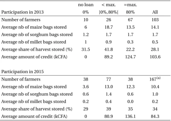
Table 3 provides detailed information for the subset of surveyed farmers who decided to participate in warrantage in 2013 and/or in 2015. Overall, farmers electing to engage in warrantage stored a large portion of harvested crops : about 28 percent on average in 2013 and 34 percent in 2015. Storage was comprised mainly of maize versus other staple food crops such as sorghum and millet. It is worth mentioning that the composition of the sample of participants corresponds with Proposition 2 of the theoretical model presented in Section 3.3. We indeed find that the participants in the scheme are divided into three groups. In 2013, 67 participants (65 percent) borrowed 80 percent of the value of their stored harvest (the maximum amount allowed for a loan), 26 participants (25 percent) borrowed less, and the remaining 10 percent chose to store without taking out a loan. The situation was slightly different in 2015, as 77 participants (50 percent) borrowed less than the maximum amount allowed for a loan, and the proportion of those who chose to store without taking out a loan was also much higher (25 percent).
Table 4 provides a simple calculation of the total cost and returns of warrantage in 2013 and 2015 for the average farmer of the sample and in each category of borrowing. In 2015, the total cost of credit
was easily offset by the rising value of the collateral: the total cost of credit for the average farmer who stored 10 bags of maize in November and borrowed 42 percent of the value of the quantity stored, was 9,100 CFA francs. This amount includes 6,240 CFA for storage costs (100 CFA per bag and per month) and 2,860 CFA for loan interests (1 percent per month). Given that the price of grain rose by 25 percent between November 2013 and May 2014 in the seven villages participating in the study, the value of the collateral increased by 28,230 CFA, which is much more than the total cost of credit.19
In 2013, the rise in grain prices was exceptionally low (only three per cent on average). As a result, the capital gain was not enough to offset the cost of warrantage. This does not mean that participants have lost money doing warrantage (they may have invested the amount borrowed in a profitable ac-tivity), but this suggests that many households are willing to pay quite a lot for storing their own grain outside of their compound.
5 Hypothetical Risk and Time Preference Data
In this section, we describe the risk and time preference data that were collected during the baseline survey. We describe the design and procedure of the experiments and we explain how we estimated the individual risk and time preferences from the experimental results. It is important to mention that we make use of hypothetical surveys instead of incentivized scoring rules, not only because it is cheaper and easier to administer to large samples, but also because we wished to avoid disturbing the operations of other activities run by the same project. In particular, running incentivized games in seven CPF villages could have caused frustration in other CPF villages that were not included in the sample used for the inventory credit study.
5.1 Risk Preferences
This section presents the estimation of the risk aversion parameter.
5.1.1 Design and Procedure of Experiments
Our experiments were built on the risk aversion experiments developed by Holt and Laury (2002). We used a multiple price list design to measure individual risk preferences. We ran two experiments offering progressively lower and higher payoffs. In each experiment, participants were presented with a choice between two lotteries of risky and safe options, and this choice was repeated nine times with 19Inflation was very low over this period: 0.53 percent in 2013, -0.26 percent in 2014, and 0.95 percent in 2015 according to the World Bank. We thus ignored it in the calculation.
different pairs of lotteries, as illustrated in Table 5. Farmers were asked to choose either lottery A or lottery B. For example, the first row of Table 5 indicates that lottery A offers a 10% probability of receiving 1,000 CFA and a 90% probability of receiving 800 CFA, while lottery B offers a 10% probability of a 1,925 CFA payoff and a 90% probability of 50 CFA payoff. More information about the script used by the experimenters is provided in Appendix.
The low payoff amounts were chosen because they were in line with the ranges of relative risk aversion parameters in previous experiments by Holt and Laury (2002) and Andersen et al. (2008), and because they amount to approximately one day’s worth of income for a non-skilled worker in Burkina Faso (around 1,000 CFA a day, i.e. about 2 USD a day in 2012), which seemed credible to respondents. In the second experiment, farmers were asked to choose between lotteries with payoffs that were ten times higher (10,000 CFA, or around 20 USD, which corresponds to the average price of a 100 kg bag of maize during the harvest season).
In practice, lotteries A and B were represented by two bags of 10 marbles of different colours: green for 1000 CFA, blue for 800 CFA, black for 1925 CFA and transparent for 50 CFA.20The composi-tion of the bags was made known to the farmers, but they could not see inside the bags. As indicated in the last column of Table 5, risk neutral individuals (r = 0) are expected to switch from lottery A to lottery B at row 5, risk loving individuals (r < 0) are expected to switch to lottery B before row 5, and risk averse individuals (r > 0) are expected to switch to lottery B after row 5.
5.1.2 Analysis of Game Results
In order to render our results comparable to previous studies, we assume a constant relative risk aver-sion (CRRA) utility function, which enables us to compute the intervals provided in the last column of Table 5. The CRRA utility function has the following form: U (x) = x1−ri/(1 − r
i), where x is the lottery prize and ri, denoting the constant relative risk aversion of the individual, is the parameter to be estimated. Expected utility is the probability weighted utility of each outcome in each row. An individual is indifferent between lottery A, with associated probability p of winning a and probability 1 − p of winning b, and lottery B, with probability p of winning c and probability 1− p of winning d, if and only if the two expected utility levels are equal:
p.U (a) + (1 − p).U (b) = p.U (c) + (1 − p).U (d),
20We conducted specific training sessions for the surveyors and equipped them with a material enabling them to explain
or, p.a 1−ri 1 − ri + (1 − p). b1−ri 1 − r = p. c1−ri 1 − ri + (1 − p). d1−ri 1 − ri which can be solved numerically in terms of ri.
We estimate risk aversion measures from these data in the following way. First, we compute the midpoint of the intervals for the low payoff and the high payoff experiments.21 We then take the average of the two interval midpoints as a measure of risk aversion. This averaging has the advantage of reducing measurement error compared to approaches based on a single experimental measure (Falk et al., 2016). We find that most farmers are risk averse, with an average of r = 0.29 (see Table 6). This average value is lower than those obtained by Harrison, Humphrey, and Verschoor (2010), who conducted similar experiments in India, Ethiopia, and Uganda.
5.2 Time Preferences
This section presents the estimation of the time-discounting parameter.
5.2.1 Design and Procedure of Experiments
We elicit the individual time-discounting parameters following Andersen et al. (2008), who incorpo-rate measures of risk aversion into the utility function curvature, which Andreoni, Kuhn, and Sprenger (2015) refer to as the double multiple price list (DMPL) method, since it relies on one multiple price list for time and one for risk.22 We built two time preference experiments in the spirit of Harrison, Lau, and Williams (2002) and Coller and Williams (1999). However, we had to adapt the content of the experiment in order to offer hypothetical pay-offs that were plausible to respondents. The two experiments differed in the time delays offered. Our design thus differs from previous studies, such as Bauer, Chytilova, and Morduch (2012) and Ashraf, Karlan, and Yin (2006), which include a binary variable indicating whether the time-discount rate elicited in the near future experiment is higher than in the distant future experiment.23
21We take the upper bound for the first interval and the lower bound for the last interval.
22Andreoni, Kuhn, and Sprenger (2015) moreover show that the convex time budgets (CTB) method, already used by
An-dreoni and Sprenger (2012), Augenblick, Niederle, and Sprenger (2015) and Giné et al. (2018), is a good alternative elicitation tool, as it is likely to increase predictive power relative to DMPL estimates at the individual level (while it make predictions close to DMPL ones at the distributional level).
23Our design does not allow us to construct such a binary variable, since the two experiments that we used differed in the time delays offered (subjects were given the opportunity to wait five days in the first experiment and one month in second experiment, and the rewards in the two experiments were not equivalent). We acknowledge that this prevents us from directly comparing our measurements to those of Bauer, Chytilova, and Morduch (2012) and Ashraf, Karlan, and Yin (2006), but it is a trade-off that we were obliged to make in order to construct a time experiment that made sense to participants. We ran a pilot study with several volunteer farmers, who were asked the same questions as in Andersen et al. (2008), where respondents are offered a choice between Option A in one month and Option B in seven months. All of the respondents in
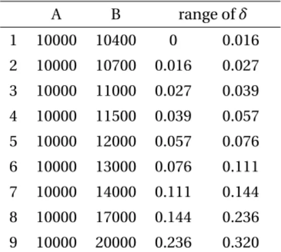
In the first experiment, farmers were invited to choose between receiving a given amount in one day’s time (option A) or receiving a larger amount in five-days’ time (option B), and this choice was repeated nine times, with increasing payoffs as option B. Table 7 displays the experiment aiming to elicit the four-day discount rate. Note that we introduced a short delay in the current income option in the earlier time frame (1 day, i.e. tomorrow rather than today). This method should control for potential confounds due to lower credibility and higher transaction costs that may be associated with future payments (Bauer, Chytilova, and Morduch, 2012; Harrison, Lau, and Williams, 2002).
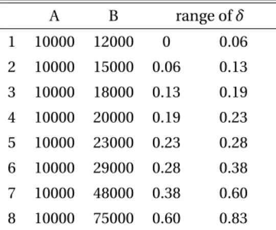
In the second experiment, farmers were invited to choose between receiving a given amount in one month’s time (option A) or receiving a larger amount in two-months’ time (option B), and this choice was repeated eight times, with increasing payoffs as option B. Table 8 displays the experiment aiming to elicit the one-month discount rate.
5.2.2 Analysis of Game Results
In order to render our results comparable to other studies, we assume that farmers have additively time-separable preferences with a per-period CRRA utility function. The form of the utility function is still: U (x) = x1−ri/(1−r
i), where x is the lottery prize and ridenotes the constant relative risk aversion of the individual. An agent is indifferent between receiving payment Mtat time t or payment Mt +1at time t + 1 if and only if:
U (w + Mt) + 1 1 + δiU (w ) = U (w) + 1 1 + δiU (w + Mt +1 )
where w is his background consumption andδiaccounts for the discount rate. Using the CRRA per-period utility function and assuming no background consumption (w = 0), we write:
M1−ri t 1 − ri = 1 1 + δi M1−ri t +1 1 − ri ,
from which we can explicitly solve forδias a function of risk aversion ri:
δi= ·M t +1 Mt ¸1−ri − 1
We use the previously estimated risk aversion parameters (ri) to calculate the interval bounds.
the pilot preferred to receive the small amount in one month, rather than the greater amount in seven months, no matter how big the greater amount was. We thus had to adapt the far-future experiment in order to offer farmers a more plausible tradeoff, which led us to build an experiment based on a delay of one month. We constructed the near-future experiment in an equally ad hoc manner. Trial and error led us to build the near-future experiment using a 4-day delay.
We then compute interval midpoints for the two time preference experiments, and take the average of these two midpoints as our estimate of an individual’s discount rate.24We find that farmers are very impatient on average, with an average discount rate of 7 percent for a four day period, i.e. 66 percent per month (see Table 6).
Our estimates of the time preference parameter fall well above previous discount rate estimates among selected populations in developed countries, which range between one and three percent per month (Harrison, Lau, and Williams, 2002). Our estimates also suggest that the farmers in our sample have higher discount rates than the rural villagers who participated in the experiments conducted by Tanaka, Camerer, and Nguyen (2010) in Vietnam and Bauer, Chytilova, and Morduch (2012) in In-dia. Our discount rate estimates also differ from those provided by Liebenehm and Waibel (2014), who conducted similar experiments with 211 households in Mali and Burkina Faso in 2007 and 2011. They report discount rates close to zero, meaning that surveyed households are extremely patient. However, they use a different experiment design (the respondents are offered a choice between im-mediate vs future rewards) and a different estimation procedure (including a noise parameter), which may have lead to lower discount rate estimates.
From the two elicited measures of impatience, we are then able to identify farmers who exhibit hyperbolic preferences. In order to construct a measure of hyperbolic discounting in accordance with the theory (see Section 3), we compute a measure of hyperbolic preferences which equals (minus) the ratio of the four-day delay discount factor and the one-month delay discount factor (converted to the equivalent discount factor for a four-day delay):
hi= −1/ (1 + δnear ) 1/ (1 + δfar)
where 1/ (1 + δnear) (resp. 1/ (1 + δfar)) refers to the four-day delay discount factor (resp. one-month
delay discount factor). A parameter hi greater than −1 indicates that the farmer is more impatient in the near future compared to a more distant future. The higher this parameter is, the stronger the hyperbolicity is.
We find that a large number of participants exhibit hyperbolic time preferences, and we obtain an average hyperbolic parameter of −1.03 (see Table 6) and a median value of −1 which indicates that half of the sample exhibits hyperbolic preferences. This result is in line with recent literature that demonstrates the existence of hyperbolic discounting based on experimental data (Ashraf, Karlan,
24In order to render the two time-discounting measures comparable, we converted the one-month discount rate to the
and Yin, 2006; Giné et al., 2018).
6 Linking preferences to warehouse inventory credit adoption
In this section, we provide an empirical framework to test Main Prediction from Section 3, stating that the optimal quantity of grain w∗increases with the hyperbolic preference parameter h. We first present the empirical model that relates warrantage adoption to risk and time preferences. We then present the main results and the robustness checks.
6.1 Econometric Framework
We estimate an empirical model where farmer i ’s decision to engage in the system is a function of her discount rate δi, level of risk aversion ri, level of hyperbolic discounting hi, other observable individual characteristics Xi, and village-by-year fixed effects:
Wi t= f (δi, ri, hi, Xi,ηt v,²i t) (7)
whereηt vis a vector of village-by-year dummies and²i tis the individual error term.
Following de Janvry and Sadoulet (2006), we selected control variables X with the aim of control-ling for household-specific features that affect production choices and hence the amount of harvest available to a farmer at the time when he makes his allocation decision (which we denote H in the theoretical model). Aside from risk and time preferences, both empirical models thus include a large set of farmer characteristics from the baseline survey, which include age and sex of the household’s head, whether he received a formal education or not, the total land area (in hectares), the number of cattle, plows, and poultry, as well as the size of the labour force (measured as the number of family members who are employed in farming activities). The village-by-year dummies control for all other factors that appear in the theoretical model: the rate of return for doing something other than war-rantage (which we denote (1 + ∆) in the theoretical model), the rate of return provided by warwar-rantage ((1 − σ)(1 + ∆)), and the interest rate of the loan (i ).
We first estimate a probit regression, in which the dependent variable, Wi t, takes on the value one if the farmer stored grain in the warehouse in year t (with or without a loan), and takes on the value zero otherwise:
The degree of hyperbolic discounting, hi, is the hyperbolic parameter as computed in Section 5.2.2. A positive coefficientλ3should then be interpreted as evidence that the more farmers exhibit
hyper-bolic time preferences, the more they use inventory credit.
We compute robust standard errors in a standard way. To test to what extent our results are robust to cluster-corrected standard errors, we moreover provide the p-values calculated by using the score bootstrap method after clustering standard errors at the village level (Kline and Santos, 2012).25 We also fit a tobit model where the left-censored dependent variable Wiis the fraction of harvest stored in the warehouse (with or without a loan). Given that 2013 was the first year in which the warrantage system was implemented and 2015 was the third year, the results for the two years may differ. In what follows, we thus report estimates for 2013 and 2015 separately, as well as estimates based on both years together.
6.2 Results
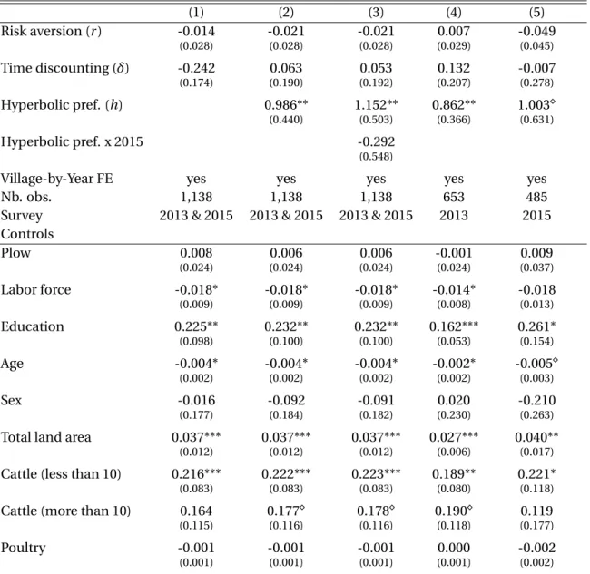
Table 9 displays the results of a probit model that links individual preferences and participation in a warrantage program. Overall, the results appear very stable. We do not find evidence that risk aver-sion and time discounting affect the probability of engaging in the warrantage system at standard levels of significance (Column 1). We do, however, find a significant and positive correlation between hyperbolic preferences and participation (Column 2). In order to examine to what extent this cor-relation may differ across years, we include an interaction term (hyperbolic parameter times year 2015) in the main model. We do not find any evidence of a stronger correlation in 2015 (Column 3), and continue to find a positive correlation between hyperbolic preferences and participation when we estimate the model using 2013 data only (Column 4) and 2015 data only (Column 5). Taking our main result (as displayed in Column 2), we calculate that a one standard deviation increase in the hyperbolic parameter is associated with a 21 percent increase in the probability of participating in warrantage. These results suggest that hyperbolic preferences may be a driver of the adoption of the warrantage system and that this effect remains stable in subsequent years.
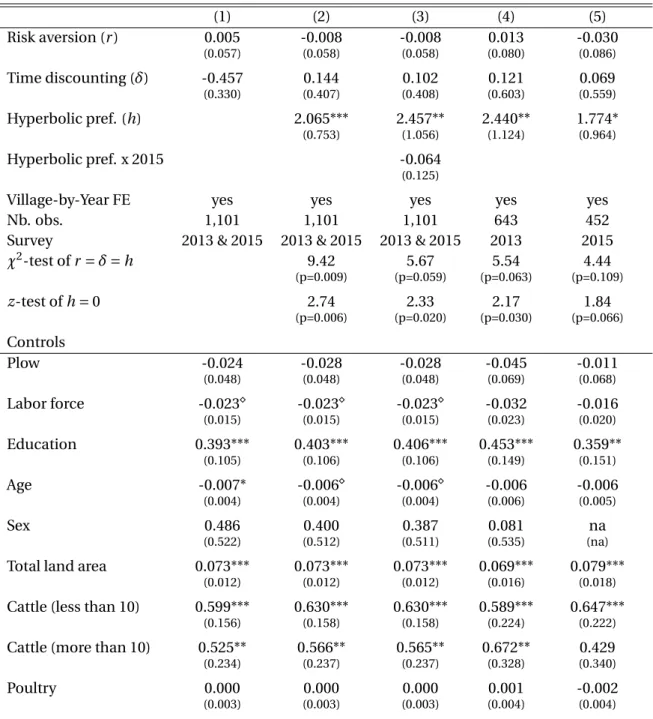
Next, we investigate whether risk and time preferences may be related to the quantity that the farmer chooses to store in the warehouse. Table 10 displays the results of a tobit model, in which the dependent variable is the fraction of the total harvest that is stored in the warehouse. We do not find any evidence of a link between risk aversion or time discounting and quantity stored (Column 1). In contrast, the correlation with the hyperbolic parameter is positive and significant (Column 2). Here
25The score bootstrap developed by Kline and Santos (2012) is an adaptation of the wild bootstrap of Wu (1986) and Liu
again, the size of the coefficient seems stable across time (Column 3), and the correlation holds when considering 2013 alone (Column 4). The coefficient is of similar size but weakly significant (the p-value is 0.11) when considering 2015 alone (Column 5).
We check whether our findings are driven by the small number of farmers who store grain in a warehouse without taking up a loan. To do so, we re-estimate the same probit model excluding those farmers and find that previous results hold, which suggest that hyperbolic preferences may be a driver of warrantage adoption even among those who ask for a loan (see Table A.1 in Appendix).
In our sample, a fraction of farmers chose only lottery B for the entire payoff series (about 15 per-cent of players in the low payoff series and up to 18 perper-cent of players in the high payoff series chose this way), which would suggest that these farmers are extreme risk-lovers. One concern that arises with these results is that these farmers did not understand how the game worked and incidentally drive our main result. Therefore, as a robustness check, we explicitly consider these risk lovers as a specific subset of the population. We augment our basic specification (Table 9) with an interaction term between the hyperbolic preference parameter and a dummy which equals one if the farmer al-ways chose the risky lottery (lottery B) in the two risk experiments (13 percent of the farmers behave this way). Our main results still hold (see Table A.2 in Appendix).
Finally, we check the robustness of the main results by including binary variables for the quintiles of the variables of interest (r ,δ, and h) instead of continuous variables. We provide the results in Table A.3 in Appendix. Main results hold.
7 Alternative explanations
In this section, we discuss alternative explanations for our results. In particular, we discuss whether individual income shocks or social pressure may explain our results. In each case, we provide argu-ments that make us confident that individual preferences are indeed linked to warrantage adoption.
7.1 Income Shocks
One could argue that our findings may arise due to an unobserved shock to income affecting both experimental measures of discounting and inventory credit adoption. Income shocks indeed have the potential to affect the way that farmers answer time-discounting questions, as well as their decisions to engage in inventory credit systems. If individuals are sufficiently liquidity-constrained, a negative shock such as a crop failure due to reduced rainfall, for example, could cause them to respond as if
they were more impatient now than in the future and simultaneously affect their savings behaviour. If this were the case, it is plausible that the correlation that we observe could be caused by these shocks rather than by a direct link between present-biased preferences and inventory credit adoption.
However, we argue that such an assumption is very unlikely to hold in our study due to the fact that a negative shock to income is likely to increase measures of hyperbolic preferences (Dean and Sautmann, 2016) and decrease savings. On the contrary, our findings suggest the existence of a posi-tive correlation between hyperbolic preferences and savings, which is in line with a demand for com-mitment.
One could also argue that most farmers who engaged in the inventory credit system chose to take a loan, which might indicate that they need cash, and this presumably due to a negative shock to income. We believe that this interpretation is unlikely to hold, as well. First, farmers who are liquidity constrained have the option to sell their crops on the market (instead of taking a loan, which amounts to 80 percent of the value of their crop only). Second, it is challenging to identify an unobserved factor that would be likely to affect both the experimental measures of a farmer surveyed in January and the need for cash during the harvest season in November.
However, despite their improbability, we cannot definitively rule out the possibility that unob-served shocks to income could affect experimental measures of time-discounting and inventory credit adoption in more complex ways. We therefore design a robustness check to address this concern. To do so, we exploit a new dataset that was collected in January 2016 from the sample of farmers who responded to the baseline survey. This follow-up survey provides the amount of maize, sorghum and millet harvested in October 2015 by participants and non-participants in warrantage in 2015. We include this variable as an additional control in the model of warrantage adoption. Because we do not have data on the 2013 harvest for farmers who did not participate in warrantage in 2013, we are able to perform this robustness test for the year 2015 only. We find that the link between time-inconsistency and warrantage adoption is robust to the inclusion of the harvest (see Column 1 of Table A.4 in Appendix). The correlation between time-inconsistency and quantity store remains of the same magnitude as before but lacks precision (see Column 2 of Table A.4 in Appendix).
7.2 Social Pressure
A final concern is that we inappropriately interpret our results as evidence that those farmers who engage in the inventory credit system are seeking a commitment savings device for its inherent ben-efits. As we point out at the beginning of the paper, there are a variety of reasons why farmers may
opt to participate in warrantage. One of these reasons is that farmers who store their crops in ware-houses are able to escape social pressure to share their harvest with kin and neighbours. Engaging in an inventory credit system may thus be an option for individuals seeking to escape this type of social pressure.
One could argue that our findings may arise due to an unobserved shock affecting both the way a farmer responds to time discounting questions and the standard of living of his neighbours. However, we include village-by-year fixed-effects in our model, which means that such covariant shocks are controlled for in our study.
8 Conclusion
Self-discipline problems may limit farmers’ ability to save grain until the lean season, which may in turn hinder their capacity to ensure the food security of their household. In developing countries such as Burkina Faso, formal commitment savings devices are lacking. We argue that warrantage systems are likely to be effective commitment savings devices in this regard.
We partnered with a rural bank and a farmers organization in order to implement a warrantage system in seven villages in Burkina Faso, and we analyse the link between farmers’ risk and time preferences and their likelihood to engage in the warrantage system. Our analysis is based on a series of hypothetical choice experiments in the field designed to elicit risk and time preferences before the beginning of the program, a baseline household survey, and two follow-up surveys carried out among participants in warrantage in the first and the third year of implementation. We found that farmers who exhibit stronger hyperbolic preferences are more likely to participate in the warrantage system than other, otherwise similar, farmers.
Inventory credit systems have been celebrated for giving farmers access to credit and, in doing so, providing them with an opportunity to overcome the “sell low buy high” phenomenon, notably because providing access to credit enables farmers to adjust their selling activities throughout the year and take advantage of seasonal price fluctuations. It is important to note that our findings do not discount the importance of the central feature of inventory credit systems, i.e. the credit itself. Instead, we emphasize the features that are likely to motivate a farmer’s decision to use such a system. Because the vast majority of farmers who entered the system chose to take out a loan, it appears that credit access serves as a strong motivation for engaging in the inventory credit system. The evidence we present here suggests that another explanation for the growing popularity of these systems may
rest in their role in helping farmers to overcome their self-discipline problems.
The results of our theoretical model moreover suggest that there may be a variety of farmer re-sponses to warrantage programs. Despite rising prices during the lean season, some farmers may not wish to store their grain in a certified warehouse over a six-month period. Specifically, these are farmers who are either not (or only slightly) inconsistent in their temporal preferences, or not sophis-ticated enough to realize that they are actually time-inconsistent and are too risk averse to take credit, as well as those who are too impatient to save their grain.
The warrantage system that was implemented in 2013 continues to function today. It should be noted, however, that the long term on-the-ground presence of the project proponent - the CPF - and the trust that characterized the relationship between farmers, the CPF and the rural bank in the study areas probably contributed to such encouraging results. In a less favorable context, many households may have been reluctant to entrust their grain to a farmer organization. It must also be recognized that the efficiency of the system can be significantly reduced when the state intervenes in the market-place via price stabilization, as occurred in 2013. Finally, beyond the participation rate, the success of the systems should also be measured through its impact on households’ standard of living and food security. More work needs to be done in order to quantify these effects.
Acknowledgements
This research would not have been possible without the full cooperation of the Confédération Paysanne du Faso. Funding for this research was provided by the European Union with counterpart funding from AGRINATURA for the Farm Risk Management for Africa project, coordinated by CIRAD.
References
Ai, C., and E.C. Norton. 2003. “Interaction terms in logit and probit models.” Economics Letters 80:123 – 129.
Aliber, M. 2001. “Rotating savings and credit associations and the pursuit of self-discipline: A case study in South Africa.” African Review of Money Finance and Banking, pp. 51–73.
Ambec, S., and N. Treich. 2007. “Roscas as financial agreements to cope with self-control problems.” Journal of Development Economics 82:120 – 137.
Andersen, S., G.W. Harrison, M.I. Lau, and E.E. Rutstrom. 2008. “Eliciting Risk and Time Preferences.” Econometrica 76:583–618.
Anderson, S., and J.M. Baland. 2002. “The Economics of Roscas and Intrahousehold Resource Alloca-tion.” The Quarterly Journal of Economics 117:963–995.
Andreoni, J., M.A. Kuhn, and C. Sprenger. 2015. “Measuring time preferences: A comparison of exper-imental methods.” Journal of Economic Behavior & Organization 116:451 – 464.
Andreoni, J., and C. Sprenger. 2012. “Risk Preferences Are Not Time Preferences.” American Economic Review 102:3357–76.
Ashraf, N., D. Karlan, and W. Yin. 2006. “Tying Odysseus to the Mast: Evidence from a Commitment Savings Product in the Philippines.” Quarterly Journal of Economics 121:635–672.
Augenblick, N., M. Niederle, and C. Sprenger. 2015. “Working over Time: Dynamic Inconsistency in Real Effort Tasks.” Quarterly Journal of Economics 130:1067–1115.
Baland, J.M., C. Guirkinger, and C. Mali. 2011. “Pretending to Be Poor: Borrowing to Escape Forced Solidarity in Cameroon.” Economic Development and Cultural Change 60:1 – 16.
Banerjee, A., and S. Mullainathan. 2010. “The Shape of Temptation: Implications for the Economic Lives of the Poor.” NBER Working Papers No. 15973, National Bureau of Economic Research. Barr, A., and G. Genicot. 2008. “Risk Sharing, Commitment, and Information: An Experimental
Anal-ysis.” Journal of the European Economic Association 6:1151–1185.
Basu, K. 2011. “Hyperbolic Discounting and the Sustainability of Rotational Savings Arrangements.” American Economic Journal: Microeconomics 3:143–71.
Basu, K., and M. Wong. 2015. “Evaluating seasonal food storage and credit programs in east Indone-sia.” Journal of Development Economics 115:200 – 216.
Bauer, M., J. Chytilova, and J. Morduch. 2012. “Behavioral Foundations of Microcredit: Experimental and Survey Evidence from Rural India.” American Economic Review 102:1118–39.
Bernheim, B.D., D. Ray, and S. Yeltekin. 2015. “Poverty and Self-Control.” Econometrica 83:1877–1911. Bester, H. 1987. “The role of collateral in credit markets with imperfect information.” European
Eco-nomic Review 31:887–899.
Bryan, G., D. Karlan, and S. Nelson. 2010. “Commitment Devices.” Annual Review of Economics 2:671– 698.
Burke, M., L.F. Bergquist, and E. Miguel. 2018. “Sell Low and Buy High: Arbitrage and Local Price Ef-fects in Kenyan Markets.” Working Paper No. 24476, National Bureau of Economic Research, April. Casaburi, L., and J. Willis. 2016. “Time vs. State in Insurance: Experimental Evidence from Contract
Farming in Kenya.” Working paper.
Coller, M., and M. Williams. 1999. “Eliciting Individual Discount Rates.” Experimental Economics 2:107–127.


![Table 9: Participation in warrantage: probit regression (1) (2) (3) (4) (5) Risk aversion (r ) 0.000 -0.013 -0.013 0.015 -0.035 (0.053) (0.053) (0.053) (0.077) (0.075) [0.997] [0.685] [0.685] [0.790] [0.472] Time discounting (δ) -0.350 0.205 0.195 0.319 0.](https://thumb-eu.123doks.com/thumbv2/123doknet/13998764.455718/38.892.116.777.168.1059/table-participation-warrantage-probit-regression-risk-aversion-discounting.webp)