Applications of a fast helmholtz solver in exploration seismology

Applications of a Fast Helmholtz Solver in

Exploration Seismology

by

Gregory Tsiang Ely

Submitted to the Department of Earth, Atmospheric, and Planetary

Sciences

in partial fulfillment of the requirements for the degree of

Doctor of Philosophy

at the

MASSACHUSETTS INSTITUTE OF TECHNOLOGY

February 2019

Massachusetts Institute of Technology 2019. All rights reserved.

Signature redacted

A u th o r ... . .. . . .. . .. . . ...

partnnt of Earth, Atmospheric, and Planetary Sciences

January 14, 2019

Certified by.

Signature

redacted

Alison Malcolm

Associate Professor, Memorial University of Newfoundland

Thesis Supervisor

Signature redacted

A ccepted by ...

...

Robert van der Hilst

Schlumberger Professor of Earth Sciences

Head of Department of Earth, Atmospheric and Planetary Sciences

MASSACHUSETTS INSTITUTE OF TECHNOLOGY

Applications of a Fast Helmholtz Solver in Exploration

Seismology

by

Gregory Tsiang Ely

Submitted to the Department of Earth, Atmospheric, and Planetary Sciences on January 14, 2019, in partial fulfillment of the

requirements for the degree of Doctor of Philosophy

Abstract

Seismic imaging techniques rely on a velocity model inverted from noisy data via a non-linear inverse problem. This inferred velocity model may be inaccurate and lead to incorrect interpretations of the subsurface. In this thesis, I combine a fast Helmholtz solver, the field expansion method, with a reduced velocity model param-eterization to address the impact of an uncertain or inaccurate velocity model. I modify the field expansion framework to accurately simulate the acoustic field for ve-locity models that commonly occur in seismic imaging. The field expansion method describes the acoustic field in a periodic medium in which the velocity model and source repeat infinitely in the horizontal direction, much like a diffraction grating. This Helmholtz solver achieves significant computational speed by restricting the ve-locity model to consists of a number of non-overlapping piecewise layers. I modify this restricted framework to allow for the modeling of more complex velocity models with dozens of parameters instead of the thousands or millions of parameters used to characterize pixelized velocity models. This parameterization, combined with the speed of the forward solver allow me to examine two problems in seismic imaging: uncertainty quantification and benchmarking global optimization methods. With the rapid speed of the forward solver, I use Markov Chain Monte Carlo methods to esti-mate the non-linear probability distribution of a 2D seismic velocity model given noisy data. Although global optimization methods have recently been applied to inversion of seismic velocity model using raw waveform data, it has been impossible to compare various types of algorithms and impacts of parameters on convergence. The reduced forward model presented in this paper allows me to benchmark these algorithms and objectively compare their performance to one another. I also explore the application of these and other geophysical methods to a medical ultrasound dataset that is well approximated by a layered model.

Thesis Supervisor: Alison Malcolm

Acknowledgments

I would first like to thank my advisor Alison Malcolm for her constant support during

my Ph.D. Completing a degree means balancing a thousand forms of doubt with brief but wonderfully moments of confidence and success. Throughout this process Alison patiently and expertly guided me to through the trials of the AAIJGerman forestaAi and helped show me what success looks like.

I would like to thank my collaborators and coauthors, Guillaume Renuade, Oleg

V. Poliannikov, David P. Nicholls, and Maria Kotsi for their advice, feedback, and support throughout my degree. I would also like to thank all of the members of my committee, Brad Hager, Bill Rodi, Sai Ravela, Shuchin Aeron, for their suggestions and questions, all of which substantially improved this thesis. Also a special thanks to past post-docs and students: Andrew Davis, who first introduced me to various methods for uncertainty quantification, and Russ Hewett for developing the wonderful PySit seismic inversion toolbox that I use throughout this thesis.

Finally, I would like to thank my family (Stephanie, Perry, and Lynette) for all of their support and putting up with me throughout this arduous process. Thank you to my father, Dick Ely, who encouraged me to pursue a Ph.D. and helped me all those years ago with my graduate applications. You are dearly missed.

Contents

1 Introduction

1.1 Fast Forward Model: Field Expansion . . . . 1.2 Uncertainty Quantification Seismic Challenges . . . .

1.3 Uncertainty Quantification Approaches . . . . 1.4 Global Optimization . . . .

1.5 Ultrasound and Bone . . . .

2 global optimization algorithms for building velocity models

2.1 Overview . . . . 2.2 Introduction . . . .

2.3 Forward Model . . . .

2.3.1 Reduced parameterization . .

2.3.2 Field Expansion . . . . 2.4 Global Optimization Methods . . . .

2.4.1 Particle Swarm Optimization 2.4.2 Simulated Annealing . . . . .

2.5 R esults . . . .

2.5.1 Simple models . . . .

2.5.2 Convergence and noise . . . . 2.5.3 Complex Examples . . . . 2.5.4 Marmousi Inversion . . . . 2.6 Discussion . . . . 2.7 Conclusion . . . . 23 . . . 26 . . . 27 . . . 29 . . . 32 . . . 33 35 . . . . 35 . . . . 36 . . . . 39 . . . . 39 . . . . 40 . . . . 43 . . . . 44 . . . . 46 . . . . 47 . . . . 48 . . . . 54 . . . . 55 . . . . 57 . . . . 60 . . . . 63

3 Uncertainty Quantification of Seismic Velocity Models and Seismic Images

3.1 Overview . . . .

3.2 Introduction . . . .

3.3 Bayesian velocity model inversion 3.4 Field expansion forward solver

3.5 Efficient posterior calculation

3.6 Results . . . .

3.6.1 Simple Anticline . . . . .

3.6.2 Gradient Migration . . . .

3.6.3 Convergence . . . . 3.6.4 Starting Model Sensitivity

3.6.5 Degrees of Freedom . .

3.6.6 Computational cost . .

3.7 Discussion . . . . 4 Imaging the Interior of Bone

4.1 Overview . . . . 4.2 Introduction 4.3 4.4 4.5 4.6 4.7 4.8 4.9 4.10 4.11 Acquisition Geometry . . . . Applications of PSO & MCMC to Ultrasound Axial: Methods & Synthetic . . . . Methods: Multiple Suppression . . . . 4.6.1 Head wave velocity analysis . . . . . 4.6.2 NMO semblance velocity analysis . .

Axial: in vivo . . . . Transverse: Methods & Synthetic . . . . Transverse: in vivo . . . . D iscussion . . . . Conclusion . . . . 65 65 66 70 72 74 81 81 85 87 90 91 92 93 97 . . . . 97 . . . . 97 . . . . 100 . . . . 100 . . . . 104 . . . . 109 . . . . 109 . . . . 110 . . . . 119 . . . . 122 . . . . 130 . . . . 130 . . . . 133 . . . . . . . . . . . . . .. . . . . . . . . . . . . . . . . . . . . . . . . . . . . . . . .

4.12 Acknowledgments . . . . 133

4.13 Appendix: Seismic techniques . . . . 134

4.13.1 Normal move-out and semblance . . . . 134

4.13.2 Kirchoff Migration . . . . 135

4.13.3 Reverse Time Migration . . . . 136

5 Conclusion 137 5.1 Future W ork . . . . 137

5.1.1 Testing assumptions and validity of assumptions . . . . 138

List of Figures

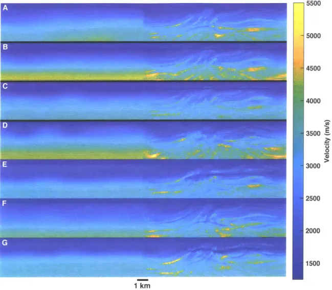
1-1 Left: Initial models used for FWI. Right: Final models after FWI. A: Inversion using the true smoothed Marmousi Velocity model. B-G:

The initial models and inversions for six different inexact initial models. 24 1-2 Diagram illustrating the seismic uncertainty framework from raw data

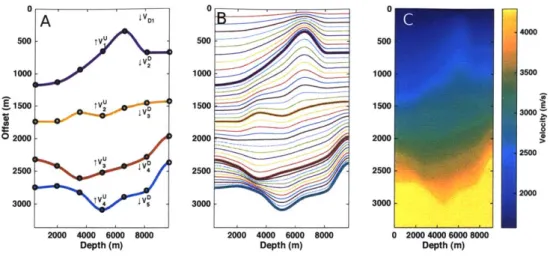
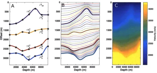
to probability distribution over a quantity of interest and final inter-pretation . . . . 25 1-3 A: Reduced parameterization diagram. B: Interpolated layer

inter-faces based on the reduced parameterization. C: Pixelized velocity

model derived from reduced parameterization consisting of piecewise constant layers. . . . . 28

1-4 Left: Log-Likelihood distribution for a fictional function. Right:

Likelihood for the same fictional problem. The local minima present in the right panel would create a problem for local optimization meth-ods but does not contribute significantly to the likelihood function and does not impact the distribution. . . . . 33

2-1 sketch of field expansion velocity model and repeating boundary con-dition s. . . . . 40 2-2 A: Reduced parameterization diagram. B: Interpolated layer

inter-faces based on the reduced parameterization. C: Pixelized velocity model derived from reduced parameterization consisting of piecewise constant layers. . . . . 41

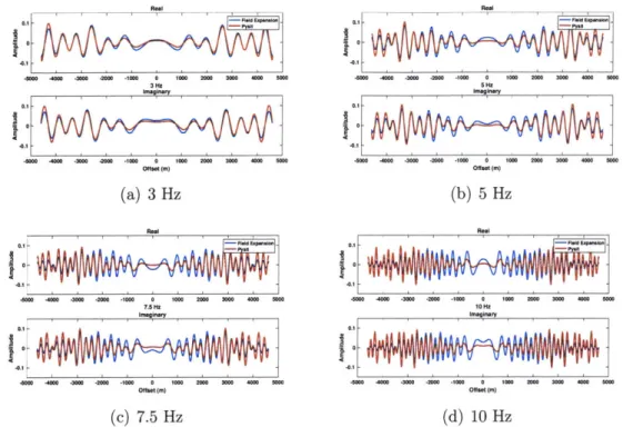
2-3 Real and imaginary components of the PySIT and field expansions

fields at several frequencies. We generate these results with a dispersion term of 2.5 x 10-2. . . . . 43

2-4 Dispersion as a function of misfit for several source frequencies. . . . 44

2-5 Marmousi constant density velocity model. . . . . 48

2-6 Single run of PSO inversion with 4 master layers. A: All initial models and the true velocity profile. B: Initial best fitting and final best velocity profile after 250 iterations. . . . . 49

2-7 Particle Swarm Optimization Convergence as a function of number of

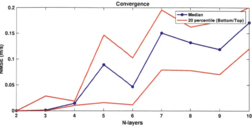
layer. . . . . 50 2-8 Simulated Annealing convergence results. . . . . 51 2-9 Convergence as a function of source frequency and number of master

layers. Median values are shown with a solid line and top/bottom 2 0th

percentile solutions are shown with dashed lines. . . . . 52

2-10 Convergence as a function of number of agents. Median values are shown with a solid line and top/bottom 2 0th percentile solutions are

shown with dashed lines. . . . . 53

2-11 Convergence as a function of maximum iteration. Median values are shown with a solid line and top/bottom 2 0th percentile solutions are

shown with dashed lines. . . . . 53

2-12 Model misfit as a function of initial guess quality. Median values are shown with a solid line and top/bottom 2 0th percentile solutions are

shown with dashed lines. . . . . 55 2-13 Illustrations of several signal to noise ratios at 5Hz. The real

compo-nent of the field are shown in blue and the imaginary in red. . . . . . 56

2-14 Model misfit as a function of Signal to Noise Ratio. Median values are shown with a solid line and top/bottom 2 0th percentile solutions are

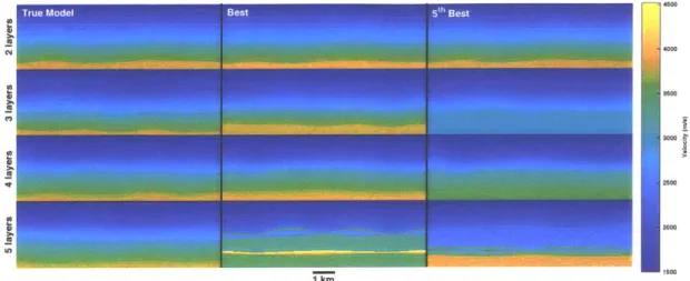
2-15 Left: True perturbed velocity models consisting of 2-5 master layers. Middle: the best fitting, lowest model NMSE. Right: The 5th best fitting (20th percentile) velocity model. . . . . 58 2-16 Convergence results for Marmousi like inversion as function of number

of m aster layers. . . . . 58 2-17 A: Data misfit between PSO inversions and the field generated from

the Marmousi model at 3Hz and 5Hz as function of number of master layers. B: Model misfit for the PSO inversion between the smoothed Marmousi model shown in Figure 2-18A left and the smoothed inverted velocity models. For both the plots the median values are shown with solid lines and the top and bottom 20th percentile solutions are shown with dashed lines. . . . . 59 2-18 Left: Initial models used for FWI. Right: Final models after FWI. A:

Inversion using the true smoothed Marmousi Velocity model. BCD: The initial models based on the best fitting, lowest data measurement error, PSO inversion at 3Hz and the resulting final models from FWI. 60 2-19 Left: Initial models used for FWI. Right: Final models after FWI. A:

Inversion using the true smoothed Marmousi Velocity model. B,C,D: The initial models based on the best fitting, lowest data measurement error, PSO inversion at 5Hz and the resulting final models from FWI. 61 3-1 A: The base velocity model consisting of 3 perturbed layers. B: The

reflector model is the same as the base model with the addition of an anticline reflector, indicated by the red arrow, in the deepest layer. The velocities within the layers are 1500, 2000, and 2500 m/s from shallow to deepest.. .. . . . . .. ... . .. . .. . . .. . . . . . 70

3-2 Left: Parameterization for gradient field-expansion. Each layer has an up and down velocity describing the velocity gradient and each boundary is described by Nq points (here 7). Center: The interpolated sub-layer boundaries between the master layers boundaries. Right: The resulting 2D velocity model. A small number of parameters (here

32) describe a complex smoothly varying velocity model that would

ordinarily require over 30,000 parameters. . . . . 74

3-3 Six representative velocity models drawn from the results of the MCMC algorithm run on the model shown in Figure 3-1. Each velocity model extends to a depth of 3,000 m and 2,500 m horizontal distance. The

resulting position of the migrated anticline reflector is also shown. . . 82

3-4 The mean velocity model from the MCMC algorithm for which six random models are shown in Figure 3-3. The solid black lines show the true position of the layer interfaces and reflector. The standard deviations of the layer boundaries are shown with the red dashed lines and the velocity uncertainties for each layer are shown. The mean position of the migrated reflector (at about 2200 m depth) and its standard deviation are also displayed. . . . . 83 3-5 Left: Histogram of migrated anticline relative height. Right:

His-togram of migrated anticline absolute depth. Both hisHis-tograms are shown with the same horizontal scale and bin size.The red vertical line denotes true values of the quantities of interest in Figure 3-1B. . 84

3-6 A: 122x384 pixel Marmousi velocity model. B: Smoothed Marmousi

model generated by applying a Gaussian low pass filtered to the original Marmousi model. C: Field expansion model based on the smoothed M arm ousi model. . . . . 87 3-7 Real and imaginary components of the measured field (blue) true

3-8 6 Velocity models drawn from the Markov-Chain; the true model is

shown in Figure 3-6C. Note that deeper sections of the velocity vary more than shallow parts. . . . . 88 3-9 Zero-offset migration using the velocity models shown in Figure 3-8

us-ing the true Marmousi reflectivity. Two potential traps are highlighted in blue and red. We characterize the uncertainty of the cross sectional area and depth of these two traps. . . . . 88 3-10 Histogram of the shallow (red) and deep (blue) anticlines depth and

area. The Metropolis-Hastings runs were initialized with the true start-ing model. The red vertical line denotes true values of the quantities of interest in Figure 3-10 . . . . 88 3-11 Convergence plot for Metropolis-Hastings inversions using 2-5 master

layers using 7 nodes per interface. Each plot shows f for the 4 quan-tities of interest as a function of iterations. the 4 models shown had the following number of degrees of freedom: 2-layers 11, 3-layers 21, 4-layers 31, and 5 layers 41. . . . . 89 3-12 Histogram of anticline depth and area using a linear gradient initial

model. The histograms using the true velocity as the starting model from Figure 3-10 are overlaid in red. The red vertical line denotes true values of the quantities of interest in Figure 3-10. . . . . 90 3-13 Left: The final R for the 4 quantities of interest as a function of bottom

velocity perturbations. Center: Histograms of anticline depth for the

a zero perturbation linear gradient starting model with overlays of

velocity perturbations of -25%,-15%,+15%,+25%. Right: Histograms of anticline Area for the a zero perturbation linear gradient starting m odel with overlays. . . . . 92

4-1 Geometry of the experiment. Each element acts sequentially as a source with the resulting wavefield recorded on all the elements. A: Transverse acquisition. B: Axial acquisition. . . . . 100

4-2 A: True velocity model used for synthetic experiment. B: Smoothed velocity model containing only the upper bone used for Kirchoff migra-tion. C: Kirchoff migration using the smoothed velocity model with true bone interfaces highlighted in red and the silicone tissue interface highlighted in black at roughly 1.5 mm. The artifacts at the source are a normal part of any imaging method that can be suppressed if necessary by muting the direct arrival. Numerous multiple reflections are present in the migrated image within the marrow; these are the lines in the image that don't correspond to true reflectors. . . . . 101

4-3 Red: Field for an in vivo measurement across the 96 transducer at a frequency of 2MHz. Blue: Simulated field using the field expansion of a synthetic model based on the in vivo imaging. The upper panel shows the real components of the field and the lower panel shows the imaginary components. . . . . 102 4-4 Dashed: The true velocity profile for the synthetic bone experiment.

solid: The best fitting velocity model for the 20 PSO inversion. . . . 102

4-5 Blue: Synthetic field across the 96 transducers at a frequency of 2 MHz without noise. Red: Simulated field with small amount of noise used for MCMC inversion. . . . . 103

4-6 Top: Three different synthetic velocity models. Middle: Synthetic common source gathers. The middle panel labeled 'marrow flood

-bone flood' shows the difference between source gathers for the -bone flood and marrow flood velocity models. Bottom: NMO semblance values of synthetic data. . . . . 107

4-7 A: Cartoon illustrating the three types of internal multiples seen when imaging in the axial geometry. B: predicted peaks for primaries and multiple in NMO semblance domain. Primaries are shown with blue circles; the potential marrow return should fall along the blue line. The

4-8 Illustration of the dictionary construction and column-wise sparsity of the weighting matrix. The figure shows propagators across several receiver indices for a single hyperbolic reflection nmo time velocity pair

(tj, Vk). For a single reflection all of the non-zero dictionary coefficients

are contained in a single column of the weighting matrix. . . . . 112

4-9 A: Raw synthetic trace with multiples present. B: denoised data with mute applied. C: f2 norm of dictionary coefficients along the receiver index direction. Red lines indicate the boundaries of the mute in the

NM O time-velocity space. . . . . 115

4-10 Migrated images with processed and unprocessed data. True interfaces are highlighted in red. The colormap is the same for all three panels with a dynamic range of 45dB. A: Migrated image using raw data. Numerous multiple returns are present that do not correspond to the true model. B: Kirchoff migrated image with only predictive decon-volution applied. Predictive decondecon-volution alone does not mitigate all of the multiples present in the data. C: Migrated image with sparse denoising and predictive deconvolution. All interfaces are estimated correctly with the exception of the lower endosteum due to using an incorrect velocity model with an infinite marrow half space shown in Figure 4-2B. The signal and clutter strengths given in Table 4.3 are cal-culated by averaging over the dashed white line and the pixels within the white box respectively. . . . . 117

4-11 In vivo migrated image of the radius. Upper images are generated with anisotropic migration. Lower images are generated with isotropic migration. (A) Migration using raw data. (B) Migration using the sparse dictionary after mute has been applied. (C) migration with hyperbolic sparse denoising and predictive deconvolution data. The Periosteum and Endosteum are labeled 'P' and 'E.' The signal and clutter intensities are reported in Tables 4.4 & 4.5 by averaging the pixel intensity over the dashed white lines (endosteum) and clutter (white box), respectively. The contrast between clutter and signal strength are given in Tables 4.6 & 4.7. . . . . 119

4-12 In vivo common source gather of the radius for a single source (A) raw data. (B) the sparse dictionary after mute is applied. (C) hyperbolic sparse denoising and predictive deconvolution. (D) The difference be-tween A and B. E the difference bebe-tween A and C. (F) The difference between D and E. The predictive deconvolution suppresses a peg leg multiple indicated by the arrows. . . . . 121

4-13 True velocity model for transverse synthetic experiments. . . . . 122

4-14 Left: snapshots of wave field propagation in transverse geometry. The

white arrow indicates the return from the bottom of the marrow and the black arrow highlights the headwave. Right: common source

gather for the simulated gather with the various arrivals and reflected signals labeled. See supplemental video synthMovie.avi . . . . 123

4-15 Transverse velocity models used for migrations. From left to right: tissue half space, bone half space, horseshoe. . . . . 123

4-16 Kirchoff migration results using the tissue half space (A), bone half space (B), and horseshoe models (C). To highlight potential reflectors below the upper endosteum the scale has been saturated for the horse-shoe migration. The signal intensity for the upper periosteum, upper endosteum, and lower endosteum were calculated by averaging along the black, white, and green lines. The clutter strength was calculated

by averaging over the pixels within the white box. The contrast

be-tween the clutter and pixel strengths are given in Table 4.8. . . . . . 125

4-17 RTM results using the tissue half space (A), bone half space (B), and horseshoe models (C). To highlight potential reflectors below the upper endosteum the scale has been saturated for the horseshoe migration. The signal intensity for the upper periosteum, upper endosteum, and lower endosteum are calculated by averaging along the black, white, and green lines. The clutter strength is calculated by averaging over the pixels within the white box. The contrast between the clutter and pixel strengths are given in Table 4.9. . . . . 126

4-18 Transverse Kirchoff (A) migration and reverse time migration (B) using the smoothed true velocity model. The signal intensity for the upper periosteum, upper endosteum, and lower endosteum are calculated by averaging along the black, white, and green lines. The clutter strength is calculated by averaging over the pixels within the white box. The contrast between the clutter and pixel strengths are given in Table 4.10. 129 4-19 Velocity models for the in vivo data in the transverse configuration.

A: tissue flood. B: bone flood. C: marrow flood. . . . . 131

4-20 Transverse Kirchhoff migrations using the velocity models in Figure 4-19. A: tissue flood. B: bone flood. C: marrow flood. The signal intensity for the upper periosteum and endosteum were calculated by averaging along the red lines. The clutter strength was calculated by averaging over the pixels within the white box. The contrast between the clutter and pixel strengths are given in Table 4.11. . . . . 131

4-21 Transverse reverse time migrations using the velocity models in Fig-ure 4-19. A: tissue flood. B: bone flood. C: marrow flood. Some structure may be visible in the horseshoe model that corresponds to the interior of marrow. The signal intensity for the upper periosteum and endosteum are calculated by averaging along the red lines. The clutter strength is calculated by averaging over the pixels within the white box. The contrast between the clutter and pixel strengths are given in Table 4.12. . . . . 132

List of Tables

1.1 Performance and tradeoffs of several types of solvers. . . . . 26

3.1 Table showing the

N?

3.2 Computation time for the field expansion forward models. . . . . 93

4.1 MCMC inversion of bone model velocities. . . . . 104

4.2 MCMC inversion of depths of bone model. . . . . 104

4.3 Synthetic signal and clutter intensity. The proposed denoising scheme improves contrast by roughly 10.8 dB. . . . . 118

4.4 In vivo isotropic migration signal and clutter strength from Figure 4-11.118 4.5 Invivo anisotropic migration signal and clutter strength from Figure 4-11. ... ... 118

4.6 Invivo Isotropic contrast between clutter and endosteum signal from Figure4-11. . . . . 118

4.7 Invivo anisotropic contrast between clutter and endosteum signal from Figure4-11. . . . . 118

4.8 Contrast between marrow clutter and interfaces for synthethic Kirch-hoff migration examples using shown in Figure 4-16. . . . . 125

4.9 Contrast between marrow clutter and interfaces for synthethic reverse time migration examples using shown in Figure 4-17. . . . . 125

4.10 Contrast between marrow clutter and interfaces for the synthetic mi-grations shown in Figure 4-18. . . . . 130

4.11 Contrast between marrow clutter and interfaces for the in vivo Kirch-hoff migrations shown in Figure 4-20. . . . . 130

4.12 Contrast between marrow clutter and interfaces for the in vivo reverse time migrations shown in Figure 4-21 . . . . 130

Chapter 1

Introduction

Uncertainty quantification (UQ) can help answer a fundamental and often overlooked question in solid Earth geoscience, 'do we know what we think we know?' The error bars found in other fields are frequently not found in geosciences, particularly seismic imaging, Geophysical imaging (particularly global scale) is unique in that the results are often not verifiable by other imaging modalities or by physically verifying the subsurface through drilling or trenching, leaving room for over interpretation of results. Without UQ we could be arguing in the noise and conflicting choices could be equally likely to be right or wrong. Significant resources are spent based on theoretical explanations of Earth's interior that could be based on erroneous or flimsy interpretations of noisy subsurface measurements. Providing error bars on the estimates could decrease the allocation of these resources from unknowable problems or aspects of the subsurface and better focus these resources on explaining aspects of the Earth that are actually constrained by observable data.

Conventional seismic inversion techniques, such as Full waveform Inversion (FWI), are typically performed with an iterative gradient based solver that can be both sensitive to an initial model and noise [97]. These methods typically result in a single solution or image of the subsurface and do not give any measures of the uncertainty, making it difficult to interpret the results. To illustrate the challenges of sensitivity to starting models, we perform a conventional FWI with a number of starting models shown in the left of Figure 1-1 using the PySit inversion toolbox [38] with 64 shots

I

Figure 1-1: Left: Initial models used for FWI. Right: Final models after FWI.

A: Inversion using the true smoothed Marmousi Velocity model. B-G: The initial

models and inversions for six different inexact initial models.

2500

2000

1500

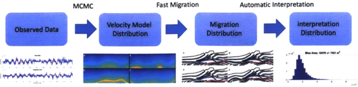
MCMC Fast Migration Automatic interpretation

Velocity Model Migration interpretation

Observed Data Distribution Distribution Distribution

Figure 1-2: Diagram illustrating the seismic uncertainty framework from raw data to probability distribution over a quantity of interest and final interpretation.

and 10 iterations at frequencies 3Hz, 4Hz, 5Hz, 6.5Hz, 8Hz and 10Hz. Although some of initial models are very close to the true blurred starting model, Figure 1-1A, the inversions result in drastically different final models and an interpreter could make a wide range of conclusions about the subsurface based on these images. Ideally one would want both an inversion scheme that is robust or independent of initial model and provides a estimate of the uncertainty of the subsurface given the observed data and noise as illustrated in Figure 1-2. In this framework the interpreter could quantify the uncertainty of some quantity of interest such as the volume or cross section of a potential reservoir.

Both global optimization methods and Markov-Chain Monte Carlo (MCMC) meth-ods can address the shortfalls of conventional solvers and provide inversions that are both robust to initial model choice and provide uncertainty quantification. However, these techniques require numerous forward solves and a reduced number of model parameters or degrees of freedom that are incompatible with conventional forward solves such as finite difference. Here we define the degrees of freedom as the number of inverted model parameters describing the seismic velocity model, i.e. number of pixels for a conventional 2D velocity model. Table 1.1 summarizes the limitations and advantages of several types of solvers used in seismic imaging and FWI. These sam-pling based UQ methods (MCMC) are inefficient, requiring hundreds of thousands of iterations, when typically less than a hundred iterations are used for conventional FWI. In this thesis we modify a Helmholtz forward solver, the field expansion method

Gradient Methods Global Optimization MCMC Number of variables: 103 - 106 102 - 103 1 - 102

Number of iterations: < 50 102 - 104 104 - 10

Robust to Local minima: No Yes Yes

Uncertainty Quantification: No No Yes

Table 1.1: Performance and tradeoffs of several types of solvers.

[58] used for modeling scattering of diffraction gratings, to rapidly simulate the

acous-tic field of seismic velocity models. This forward solver is several orders of magnitude faster than conventional seismic forward solvers, allowing us to perform both global optimization and MCMC sampling within a few hours instead of the weeks or months required for conventional solvers.

1.1

Fast Forward Model: Field Expansion

The methods presented later in this thesis rely on solving the Helmholtz equation thousands or hundreds of thousands of times for a realistic seismic velocity model. This number of forward solves would be infeasible with conventional forward models used in the seismic community. We combine a fast method of solving the Helmholtz equation [58] with a reduced parameterization that can accurately characterize the velocity model with a fraction of the number of variables typically used to describe a 2D velocity model. In this parameterization, illustrated in Figure 1-3, we restrict the velocity model to consist of a series of 'master layers' in which the velocity varies smoothly along a linear gradient. This parametrization has been used throughout seismology [107, 26, 16]. Because we artificially choose the number of layers and the number of interpolated points controlling the shape of the interface, this parameteri-zation may be overly restrictive. Advanced UQ methods could be used to marginalize across all number of layers and find the reduced parameterization needed to describe the velocity model distribution for the field expansion model [12]. In addition other methods, such as level sets [561, could be used to define the interface shapes and boundaries of the velocity model instead of splines.

the velocity model in that we restrict the velocity model to consist of non overlapping layers with limited lateral variations and only consider acoustic (non-elastic) wave propagation. However, these simplifications allow us to perform the high number of forward solves for sampling based UQ methods. This thesis is unique in that it exploits the structure of the parameterization to generate fast forward solves of the Helmholtz equation as detailed in Chapter 2. Previous work has typically combined this or other reduced parameterization with a conventional forward solve [16] that fails to take advantage of faster wave simulations made possible by the reduced model. Without this approach, it would be impossible perform a fully non-linear sampling of the posterior distribution. Although there are numerous UQ methods that are faster and more sophisticated than those presented in Chapter 3, establishing what these non-linear distributions actually are for seismic imaging has previously not been possible. Once this baseline has been established, more advanced methods that typically make some sort of approximation and further exploit the structure of the problem can now be compared to a known 'true' distribution. In addition, the speed of forward model and parameterization allows us to compare several types of global optimization algorithms against each other that would be impossible to compare without the ability to solve the forward model rapidly as done in Chapter 2.

1.2

Uncertainty Quantification Seismic Challenges

Uncertainty quantification is invaluable for building knowledge but is it rarely done. There are numerous computational, visualization, and interpretation challenges that prevent UQ from widely being adopted and the perceived reward may be too small to overcome these challenges. In addition, telling a story with UQ is difficult and can be less compelling. Instead of a single objective history of what happened we have a population of unreliable narrators describing their versions of the past. In the context of seismic imaging and velocity model building, UQ describes the distribution of velocity models and seismic images given recorded data. In the fullest extent this would mean characterizing a non-linear distribution consisting of thousands or

0 0 0 4000 500 A500 1000 1000 - 1000 3500 1500 - 15W 3000 o02000 2000 2000 2500 2500- v 4V 2500 2500 2000 3000 - T -I 300 3000 300000 V L 2000 4000 6000 8000 2000 4000 6000 8000 0 2000 4000 6000 8000

Depth (m) Depth (m) Depth (m)

Figure 1-3: A: Reduced parameterization diagram. B: Interpolated layer interfaces based on the reduced parameterization. C: Pixelized velocity model derived from reduced parameterization consisting of piecewise constant layers.

millions of variables, one for every pixel or voxel in a velocity model. Clearly analyzing this uncertainty in high dimensional space would be challenging.

Even if it is possible to calculate uncertainty on such a large variable space, it is extremely challenging to display this uncertainty in a meaningful way and it is unclear how to use this uncertainty estimate in downstream processing. Putting error bars on an image is not a straight forward task. If one assumes that uncertainty of a seismic velocity model is uncorrelated from pixel to pixel and thus can be described completely

by the diagonal entries of a covariance matrix, it would be possible to display this

as an image similar to an illumination map. However, these visualizations would not show any of the correlated errors that can be extremely significant, especially in height. For example, as shown in Chapter 3 an erroneously high velocity or low velocity region can causes areas below to shift up and down but relative height or shape may be far more consistent. Alternatively as proposed by [88] and shown in Chapter 3 we can instead view a series or movie of representative samples drawn from distribution of subsurface imaging to get a general sense of uncertainty.

Conveying a general sense of uncertainty in an image is extremely challenging and the UQ framework is likely the most useful when asking a specific question about the subsurface such as possible existence of hotspot, the angle of subduction slab, or the

volume of potential trap where the UQ can be reduced to a low dimension. Figure 1-2 summarizes this workflow from raw data to defining uncertainty over a quantity of interest. However, asking a specific question about the subsurface requires a general sense of what is in the Earth and global optimization methods described in Chapter 2 may be a better way to get an initial maximum Likelihood estimate or best guess solution of the subsurface. Once this 'best' image is initially analyzed and interpreted, specific questions can be formulated and we can develop a definitive UQ framework to answer those questions.

Even if you are able to generate an UQ estimate for the velocity model and seismic image, most seismic imaging questions require human interpretation of a final image. If we adopt an ensemble approach in which the distribution is characterized by a col-lection of samples, we typically need to interpret thousands of models to characterize uncertainty for a single velocity model. This approach is likely too onerous and some form of automation is needed to develop a full framework for seismic imaging UQ. In chapter 3 we use a very simple form of automatic interpretation that is relatively easy to implement and execute on thousands of models. Alternatively Machine Learning (ML) has recently been used to automate several interpretation tasks [35, 101]. In-stead of simply using ML as a means of speeding up interpretation, ML could enable interpretation on tens of thousands of images that would be infeasible to do manually. This could allow for performing UQ on highly subjective interpretations that would be impossible to automate in a conventional manner.

1.3

Uncertainty Quantification Approaches

Although later in thesis we choose to use the adaptive Metropolis-Hastings algorithm

[36] for UQ, there is a large variety of UQ methods [84, 48] many of which may be superior for UQ in terms of required evaluation of the forward model, number of degrees of freedom, and estimation of the dimensionality or subspace of the probability distribution.

con-verge than other UQ techniques, however these methods make fewer assumptions about the structure of the underlying distribution and perform well in moderate to high dimension [6]. In addition, they are frequently used to to estimate the refer-ence distribution to compare against more advanced UQ methods as done in [59]. Since the structure of the velocity model distributions in seismic imaging are not well known, simple and robust algorithms such as the adaptive Metropolis-Hastings are ideal for determining the characteristics of these distribution. In addition, Hamilto-nian MCMC would at first appear to be a more attractive and easy to implement form of sampling that should perform better in higher dimension than the adaptive Metropolis-Hastings algorithm [62]. However, Hamiltonian MCMC requires the cal-culation of the gradient of the likelihood function and unlike conventional forward solvers, the field expansion is not self adjoint and the calculation of the gradient can be computationally expensive. It may be possible to adapt the method used in [57] to efficiently calculate the gradient for some or all of the variables but this approach is less straightforward than using the adjoint state method [66] to calculate the gra-dient. In addition, there are methods that attempt to estimate the gradient based on previous evaluations to improve mixing and accelerate convergence [81, 11]. Particle filters or sequential Monte-Carlo methods [18] could also be well suited for uncer-tainty quantification of time lapse seismic in which a sequence of measurements are presented and could significantly reduce computational cost in this context.

In addition to sampling based methods, techniques based on suitable approxima-tions of the forward model or likelihood function can drastically reduce the cost of uncertainty quantification over sampling based methods. Polynomial chaos expan-sion methods in which the probability distribution is characterized by a truncated series can be used to quantify uncertainty for moderate dimensional problems with far fewer evaluations of the forward model [20, 102]. However, these methods be-come computational expensive when the dimension of the problem exceeds 20 [14]. These methods may be more appropriate in the context of target oriented FWI in which the uncertainty of only a small part of a velocity model is being estimated and the dimensionality of the problem could be small [46]. In addition, it is possible

to use machine learning techniques to approximate a surrogate model of the wave or Helmholtz equation and evaluate this surrogate model significantly faster than is possible with conventional wave equation solvers [13, 83]. Optimal transport maps provide another possible method of significantly reducing the computational cost by projecting the complex probability distribution into a domain in which the distri-bution is much simpler (i.e. Gaussian) [80]. These methods can be combined with sampling methods to drastically reduce computational cost [59, 64].

In this thesis we choose to use the adaptive Metropolis-Hastings algorithm to sample from the posterior velocity model distribution. Although this is fairly simple and slow to converge sampling method, it was previously infeasible to generate this distribution with current forward models. Now that we established and validate the distribution, albeit in a slow way, we can now explore the more advanced techniques and objectively compare them to the 'true' distribution. Markov Chain Monte Carlo

(MCMC) methods and other non-linear UQ methods typically require far fewer

de-grees of freedom [36], 10s to 100s at most, than those used to describe even a modest

2D or 3D velocity model. In order to provide an estimate of the velocity model

distri-bution typically one of two assumptions are made: Gaussian distridistri-bution or reduced parameter space. First, one can assume that the velocity model distribution is well approximated by a Gaussian. This assumption essentially linearizes the wave equa-tion about some point estimate and the covariance of the Gaussian matrix can be described through the Hessian [109]. One problem with this assumption is that it is likely impossible to store the full covariance matrix as this is of size ntxels where

npixels is the number of pixels or voxels in the velocity model. However, there are

methods that can draw representative solutions from a Gaussian distribution with-out explicitly generating a covariance matrix [25]. Although this approximation is computationally feasible, the assumption of a Gaussian distribution does not appear accurate as demonstrated in Chapter 3. However, this assumption may be valid in low-noise scenarios in which the minima are well behaved or in scenarios where you have an excellent initial model, like time lapse seismic.

de-scriptions of the velocity model distribution, the number of degrees of freedom must be reduced significantly. Once the degrees of freedom are reduced, this parameter-izations can be combined with fast forward models to run the tens or hundreds of thousands of forward solves needed to converge to the true velocity model distribution using MCMC. Depending on the particular problem, numerous methods exist to de-crease the degrees of freedom [110, 16, 15, 82]. However, the challenge in reducing the

degrees of freedom is choosing a parameterization that accurately models the physics of the inverse problem with fewer variables. The main drawback of this approach is that by design the fidelity of the model is significantly lower than the pixelized or voxelized models typically used in seismic imaging, and the scale of uncertainty attempting to be characterized may be significantly smaller than the reduced param-eterization. Although numerous researchers have adopted this approach, few have attempted to find reduced parameterizations that allow for an accelerated forward solver such as the one explored in this thesis.

1.4

Global Optimization

In some cases performing a rigorous non-linear UQ analysis may be unnecessary or impossible to perform due to slowness of the forward solver or requiring a model have more degrees of freedom than possible for UQ. In addition, if there is little noise in the observed data, having a maximum likelihood estimate or best fitting model may be sufficient as illustrated in Figure 1-4. For example, once the maximum likelihood estimate is found, a local Gaussian approximation of the distribution in Figure 1-2 would likely be sufficient and MCMC methods be unnecessary. However, the wave and Helmholtz equations are non-linear and even in low noise environments local minima will trap gradient based solvers and lead to premature convergence to an incorrect answer.

In the second chapter, we explore the application of global optimization methods to estimate an initial starting model without an initial guess. Furthermore, the speed of the forward solver allows us to benchmark several existing global optimization

al-log likelihood

9

-

7-3

--- 8 6 4 C0. .2 (.106 0.8 1

Figure 1-4: Left: Log-Likelihood distribution for a fictional function. Right: Like-lihood for the same fictional problem. The local minima present in the right panel would create a problem for local optimization methods but does not contribute sig-nificantly to the likelihood function and does not impact the distribution.

gorithms and study the effects of various parameters on convergence. Due to the cost of forward modeling steps typically used in seismic imaging, numerical studies of pa-rameter impacts on global optimization methods have not been explored. In addition, we demonstrate how these inverted starting models can impact the final FWI results. In this chapter we also discuss in detail how to modify the field expansion method so that it can generate data that are comparable to finite difference simulations.

1.5

Ultrasound and Bone

In the fourth chapter we attempt to apply the methods presented in the first two chapters to real data from medical ultrasound. This data was originally desirable as its layered geometry, lack of direct arrival, and lack of surface multiples made it an attractive data set to apply my techniques. However, the acquisition geometry (under sampled in the offset direction) and unmodeled physics (strong anisotropy), and high noise made these techniques difficult to apply and generate good results. While attempting to apply the more exotic techniques developed in the first two chapters of the paper, I explored the application of a number of conventional seismic techniques to the data set in order to understand what was actually contained in the datasets. In an attempt to understand the data and difficulty of imaging geometry we developed several novel techniques to image the interior of bone that are presented

39M

2.5 104' likeli .hood

Chapter 2

global optimization algorithms for

building velocity models

2.1

Overview

In this chapter, we use a fast Helmholtz solver with global optimization methods to estimate an initial velocity model for full-waveform inversion based on raw recorded waveforms. More specifically, we combine the field expansion method for solving the Helmholtz equation with a reduced parameterization of the velocity model allowing for extremely fast forward solves of realistic velocity models. Unlike conventional Full Waveform Inversion that uses gradient based inversion techniques, global optimization methods are less sensitive to local minima and initial starting models. However, these global optimization methods are stochastic and are not guaranteed to converge to the global minima. Because our adaptation of the field expansion method is so fast, we can study the convergence of these algorithms across parameter choice and starting model. In this chapter we compare two commonly used global optimization methods, particle swarm optimization, and simulated annealing, and examine the limitations of these algorithms and their dependence on choice of parameters. We find that

PSO out-performs SA and that PSO converges reliably for noisy data provided the

number of parameters remains small. In addition, using this methodology we are able to estimate reasonable FWI starting models with higher frequency data.

2.2

Introduction

Most seismic techniques such as imaging, rely on a velocity model inverted from noisy data through a non-linear inverse problem. These inverted velocity models may be inaccurate and lead to incorrect interpretations of the subsurface. For example, an erroneously fast or slow section of a velocity model could cause a syncline structure to appear as an anticline and be incorrectly interpreted as a potential trap. Full Waveform Inversion (FWI) and other gradient based methods will converge to local minima [99] and will lead to inaccurate velocity models if initiated with an inaccurate starting model [97]. In recent years UQ methods have been applied to the FWI prob-lem in order to mitigate the impact of local minima and provide a more probabilistic interpretation of the sub surface [82, 109, 69]. See [63] for a discussion of importance of risk assessment and Uncertainty Quantification (UQ) in seismic imaging. These methods allow for an informed decision about the reliability of the subsurface image and aid in risk estimates for drilling a potential well. However, these methods either require hundreds of thousands of wave equation forward solves to converge and give accurate error estimates of subsurface parameters [23] or use local approximations of a Gaussian to approximate the uncertainty [25]. The number of forward solves re-quired for MCMC is likely infeasible for many seismic imaging problems and forward models. In addition in low noise scenarios there many only be a single region of high probability and MCMC techniques may be unnecessary. Instead, global optimization methods are an attractive alternative as they require far fewer forward solves and provide an estimate of the best fitting model (maximum Likelihood) at a fraction of the number of forward solves needed for UQ and yet can still avoid being trapped by local minima.

In recent years global optimization methods such as Simulated Annealing (SA)

[16, 27, 75] and Particle Swarm Optimization (PSO) [22, 78] have become popular

methods of calculating an initial velocity model. These methods can be an alter-native or to supplement conventional methods of building velocity models such as tomography, NMO velocity analysis or very low frequency FWI [100]. Conventional

initial velocity building methods typically rely on gradient based minimization and often require the manual picking of arrival times or picks in semblance space. By contrast, global optimization methods, although not guaranteed to converge to the global minima, are far more robust to local minima and frequently do not require the calculation of a gradient, reducing memory constraints and algorithmic complexity. However, starting models, frequency, and other parameter choice can have a signifi-cant impact on the convergence of these algorithms. Although these algorithms re-quire significantly fewer iterations than UQ algorithms, rigorous comparison rere-quires numerous global optimization runs and thousands or tens of thousands of forward solves. In addition due to the stochastic nature of these algorithms, two different runs with the same starting model can converge to different finals models, requiring even more simulations to understand performance. Due to the computational cost of most forward solvers, previous work has been unable to accurately characterize these impacts and benchmark these algorithms as significant simplifications were necessary to control this computational cost. For example, [74] use analytical solutions to test problems as well as the ID wave equation to compare global optimization algorithms. In another attempt to make the problem computationally tractable, previous work has typically shown performance with one or only a few starting models when tens or hundreds of runs are necessary to generate a statistical model of convergence and accurately compare one algorithm to another [71]. Studies in the global optimization literature use test functions that are extremely fast to evaluate but are not repre-sentative of local minima found in FWI and seismic imaging. Other work combining global optimization methods and FWI have lacked a sufficiently fast test function that accurately accounts for the physics of seismic inversion in 2D.

In this chapter, we use the reduced model parameterization of velocity models introduced in [26, 107] and [16] combined with two global optimization methods to estimate an initial velocity model. Due to the rapid speed of our forward model and our approach we can quantitatively characterize the limits on the number of degrees of freedom, importance of initial guesses, choice of tuning parameters, comparison of different global optimization methods and impact of source frequency. These

com-parisons, would be impossible with conventional slower finite difference solvers. From the numerical studies presented in this chapter we are able to draw several conclusions about the performance of global optimization methods for FWI and what may impact the likelihood of finding a good initial model. Although the FWI problem is known to be more prone to local minima at higher frequency [99], we find that source frequency does not significantly decrease the likelihood of convergence and a good starting model can be found with a relatively high frequency of 5 or 8 Hz from raw waveform data. This suggests we could build initial background velocity models with much higher frequencies than are typically used. We also find that the accuracy of the initial starting models did not have a significant effect on the likelihood of converging to the correct model. From our results we find that only having an extremely accurate initial model improved the likelihood of convergence and that if the initial model(s) are outside this range the likelihood of convergence is very weakly dependent of starting model. This suggests that only if the initial model is in the basin of attraction of the global minima are we guaranteed to converge to the true solution and outside of this range the global optimization methods are equally likely to find an accurate solution independent of starting model. In addition, we find that our implementation of Particle Swarm Optimization (PSO) out performs Simulated Annealing (SA) and is able to find a more accurate initial model with the same number of forward solves.

The remainder of the chapter is organized as follows. We first describe a reduced parameterization of the velocity model that is compatible with the field expansion forward solver. We then demonstrate that this first forward model and parametriza-tion can yield comparable results as finite difference simulaparametriza-tions if modificaparametriza-tions are made to the forward solver. Second, we describe the two global optimization methods used in the chapter: Particle Swarm Optimization (PSO) and Simulated Annealing

(SA). Finally, we demonstrate our inversion on several synthetic models of varying

complexity to determine the limitation on number of degrees of freedom, choice of initial model, and iterations needed. The field expansion method achieves significant computational saving through restricting the velocity model to consist of series of

non-overlapping layers. Although this parameterization severely restricts the velocity models we can simulate, we find that the model is sufficiently accurate to estimate initial models for FWI as demonstrated later in the chapter.

2.3

Forward Model

Unlike gradient based minimization methods, global optimization and uncertainty quantification methods require far fewer degrees of freedom, tens vs thousands. In this section we briefly describe the reduced parametrization previously used by the authors in [23] for uncertainty quantification. The reduced parameterization is com-patible with the field expansion method [58], allowing for extremely rapid forward modeling of the Helmholtz equation. We briefly describe the field expansion method and the modifications we make to the forward solver to mitigate several of the artifacts inherent to the field expansion method.

2.3.1

Reduced parameterization

The field expansion method is able to achieve rapid forward solves by heavily restrict-ing the velocity model to consists of a number of non-overlapprestrict-ing piece-wise constant layers as shown in Figure 2-1. Although the Earth has often been approximated by series of layers, this parameterization of the velocity model is likely too restrictive for most applications. In addition, parameterizing each layer individually as a variable would require many more degrees of freedom than is compatible with global optimiza-tion methods. A more realistic parameterizaoptimiza-tion introduced in [26] is to approximate the Earth as a series of curved interfaces with a velocity gradient between the many interfaces. This parameterization, illustrated in Figure 2-2 allows for complex velocity models with only a few degrees of freedom and has successfully been used for global optimization [16], tomography [107], and for uncertainty quantification [23]. [16] use a similar parameterization for global optimization with finite difference methods and thus are significantly limited in computation time. Through combining this parame-terization with the field expansion, we can invert the velocity models in a fraction of

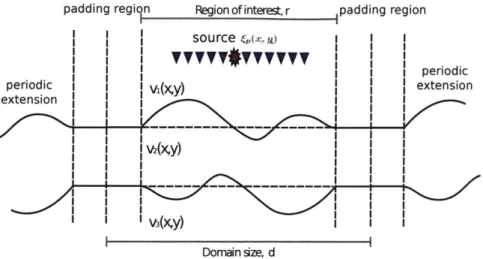
padding region Region of interestr padding region source c(x )I I | I periodic periodic I extension I I I I I v13(Xy) Domaein size, d

Figure 2-1: sketch of field expansion velocity model and repeating boundary

condi-tions.

the time. [23] argues that the field expansion forward solver is roughly 30 to 40 times faster than finite difference methods depending on the model complexity.

We build a perturbed layered velocity model following from [23] and illustrated

in Figure 2-2A. The velocity model consists of M master interfaces each with Nq

control points which control the relative height of interface across horizontal position. The full position of interfaces are interpolated with cubic splines between the control points. The velocity inside layer i from interface i - 1 to i is a linear gradient from

V, to Vd increasing with depth. Although we cannot achieve a true gradient with the piece-wise constant constraint of the field expansion, we can approximate this

gradient by dividing each layer into numerous constant velocity sub-layers as shown

in Figure 2-2B3. This parameterization allows us to generate fairly complex velocity

models with a limited number of parameters. For a model with 4 layers and 7 control points per interface we require only 32 degrees of freedom compared to the tens of

thousands needed for a pixelized velocity model as shown in Figure 2-2C.

2.3.2

Field Expansion

In this section we briefly describe the field expansion method for solving the Helmholtz equation, see [58, 22] for a more detailed description of the method. The field

ex-0 . . . .0 0 0A 0 1000 - 1000 -- 1000 30 1Soo VU 1500 1500 4000 2 V 2000- 2000 2000 2500 2500 3 4 2500 2500 U 2000 3000 - T V₅ 3000 - 3000 2000 4000 6000 8000 2000 4000 6000 8000 0 2000 4000 6000 8000

Depth (m) Depth (m) Depth (m)

Figure 2-2: A: Reduced parameterization diagram. B: Interpolated layer interfaces based on the reduced parameterization. C: Pixelized velocity model derived from reduced parameterization consisting of piecewise constant layers.

pansion method solves the Helmholtz equation for periodic boundary conditions as illustrated in Figure 2-1. The method achieves significant computational saving by taking the analytic solution to the scattered field for a series of flat horizontal layers and then using series expansions to calculate the scattered field for non-flat interfaces. The source and model repeat infinitely in the horizontal direction. These boundary conditions and source configurations vary significantly from the boundary conditions typically used in seismic imaging. In the following section we discuss how we

mod-ify the velocity model and field expansion method to make the results comparable to

finite difference methods with perfectly matching layers frequently used in seismology. In the field expansion the field within a vm(x, y) layer subject to a periodic point source is given by p(XY) = ei(P(XXO)+PYYO(2.1) 2id _OP where, Vk2 -& a22 2 ap = a + (27r/d)p = miP (2.2)