en fr

(1)

HAL Id: tel-01426001

https://tel.archives-ouvertes.fr/tel-01426001

Submitted on 4 Jan 2017

HAL is a multi-disciplinary open access

archive for the deposit and dissemination of sci-entific research documents, whether they are pub-lished or not. The documents may come from

L’archive ouverte pluridisciplinaire HAL, est destinée au dépôt et à la diffusion de documents scientifiques de niveau recherche, publiés ou non, émanant des établissements d’enseignement et de

Event-Based Feature Detection, Recognition and

Classification

Gregory Kevin Cohen

To cite this version:

Gregory Kevin Cohen. Event-Based Feature Detection, Recognition and Classification. Robotics [cs.RO]. Université Pierre et Marie Curie - Paris VI; University of Western Sydney, 2016. English. �NNT : 2016PA066204�. �tel-01426001�

(2)

University of Pierre et Marie Curie

Western Sydney University

Doctorate school: SMAER

Institut de la vision - Vision and Natural Computation BENS Group – The MARCS Institute

Event-Based Feature Detection, Recognition and

Classification

Defended by Gregory Kevin Cohen

Discipline/Speciality

Robotic

Supervised by:

Pr. Ryad Benosman, Pr. André van Schaik and Pr. Jonathan Tapson

Defended 5

th

_{September 2016}

Defense committee:

Pr. Barnabé Linares-Barranco, Instituto de Microelectrónica de Sevilla Reviewer Pr. Elisabetta Chicca, Universität Bielefeld Reviewer Pr. Bruno Gas, Institut des Systèmes Intelligents et de Robotique, UPMC Examiner Pr. Jonathan Tapson, The MARCS Institute, Western Sydney Univeristy PhD advisor Pr. Ryad Benosman, Institut de la vision, Université Pierre et Marie Curie PhD advisor Pr. André van Schaik, The MARCS Institute, Western Sydney Univeristy PhD advisor

(3)

Abstract

One of the fundamental tasks underlying much of computer vision is the detection, tracking and recognition of visual features. It is an inherently difficult and challenging problem, and despite the advances in computational power, pixel resolution, and frame rates, even the state-of-the-art methods fall far short of the robustness, reliability and energy consumption of biological vision systems.

Silicon retinas, such as the Dynamic Vision Sensor (DVS) and Asyn-chronous Time-based Imaging Sensor (ATIS), attempt to replicate some of the benefits of biological retinas and provide a vastly different paradigm in which to sense and process the visual world. Tasks such as tracking and object recognition still require the identification and matching of local visual features, but the detection, extraction and recognition of features requires a fundamentally different approach, and the methods that are commonly applied to conventional imaging are not directly applicable.

This thesis explores methods to detect features in the spatio-temporal information from event-based vision sensors. The nature of features in such data is explored, and methods to determine and detect features are demonstrated. A framework for detecting, tracking, recognising and classifying features is developed and validated using real-world data and event-based variations of existing computer vision datasets and benchmarks.

The results presented in this thesis demonstrate the potential and effi-cacy of event-based systems. This work provides an in-depth analysis of different event-based methods for object recognition and classifi-cation and introduces two feature-based methods. Two learning sys-tems, one event-based and the other iterative, were used to explore the nature and classification ability of these methods. The results demon-strate the viability of event-based classification and the importance and role of motion in event-based feature detection.

(4)

Acknowledgements

The author would like to thank his primary supervisors, Andr´e van Schaik, Jonathan Tapson, and Ryad Benosman for their tireless sup-port, constant stream of ideas and inspiration, and for imparting their interest and passion for their fields.

Additionally, the author would like to thank Philip de Chazal for his insights and guidance, Klaus Stiefel for countless fascinating discus-sions, Sio Leng and Christoph Posch for all their ideas, help, and for assisting the author with navigating the French bureaucratic system and to Francesco Galluppi and Xavier Lagorce for their insights and their friendship.

A special acknowledgement needs to be extended to Garrick Orchard, who put up with a never-ending stream of questions, provided the author with an opportunity to visit his lab in Singapore, and phys-ically saved his laptop more than once. Also, the author would like to thank David Valeiras for his unwavering enthusiasm and for many after-hour discussions in Singapore.

Personally, the author could not have completed this work without the support and friendship of Andrew Wabnitz, David Karpul, Mark Wang, Paul Breen, Gaetano Gargiulo, Tara Hamilton, Saeed Afshar, Patrick Kasi, Chetan Singh Thakur, James Wright and Yossi Buskila. Finally, the author would like to thank his family for their unwavering support, optimism and encouragement.

(5)

List of Figures

2.1 Inter-device communication using Address Event

Repre-sentation (AER). The neurons in Device 1 are assigned a unique address by the arbiter, and when they spike, an event is sent serially down the AER data bus that connects the two devices together. A decoder on the second device reconstructs the spike and makes it available to the target neurons. This figure has been adapted from [1]. . . 11

2.2 Functional diagram of an ATIS pixel [2]. Each pixel in the

ATIS camera contains both a change detector circuit (CD) and an exposure measurement circuit (EM). The CD circuitry generates events in response to a change in illumination of a certain magni-tude (specified by an externally configurable threshold). The CD circuitry can also be configured to trigger the EM circuitry, which encodes the absolute light intensity on the pixel in the inter-spike interval between two spikes. Each pixel operates asynchronously, eliminating the need for a global shutter and is capable of individ-ually encoding change events and events containing illumination information. These events are generated and transmitted asyn-chronously from each pixel in the sensor. . . 14

2.3 Example output from the ATIS sensor showing the TD

output (left) and the EM output (right) for a typical out-door scene [3]. The scene represents a person walking away from the camera, with the background remaining static. The TD im-age on the left was constructed by buffering all events over a fixed time period and displaying a black or white dot for pixels which have recently experienced an increase or decrease in intensity re-spectively. The EM image on the right shows the absolute pixel intensity, which receives pixel value updates whenever the TD cir-cuit detects a change. . . 15

(9)

List of Figures

2.4 Structure of a typical 3-Layer LSHDI Network. The inputs

are projected through a set of random weights to a larger hid-den layer of neurons, each implementing a non-linear activation function. The outputs of these neurons are linearly weighted and summed for each output neuron. . . 23

2.5 Topology of the Synaptic Kernel Inverse Method (SKIM)

[4]. Each input layer neuron (left) will be an input from a separate pixel. At initialisation, the static random weights and synaptic kernels are randomly assigned and they remain fixed throughout the learning process. During learning, the output weights in the linear part of the system are solved to minimise the error between the system output and the desired output. . . 27

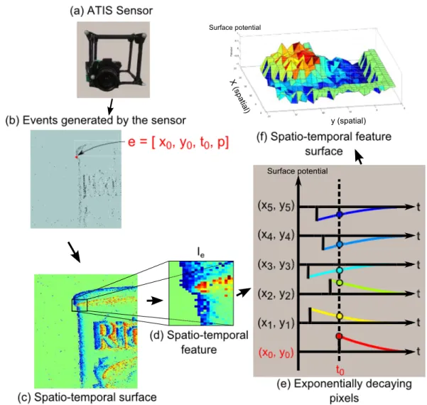
3.1 Construction of a spatio-temporal time surface and

fea-tures from the event-based data. The time surface encodes the temporal information from the sensor into the magnitude of the surface as each event arrives. The ATIS sensor shown in (a) and attached to a rig with fiducial markers for 3D tracking, generates a stream of events (b) as the camera is moved across a static scene. When an event occurs, such as event e from the pixel (x0, y0) at

time t0, the value of the surface at that point is changed to reflect

the polarity p → {−1, 1}. This value then decays exponentially as t increases, yielding the spatio-temporal surface shown in (c). The intensity of the colour on the surface encodes the time elapsed since the arrival of the last event from that pixel. A spatio-temporal fea-ture consists of a w ×w window centred on the event e, as shown in (d). An example of the decaying exponentials in the feature that generate the time surface at t = t0 is shown in (e). The

spatio-temporal feature can also be represented as a surface, as shown in (f). . . 31

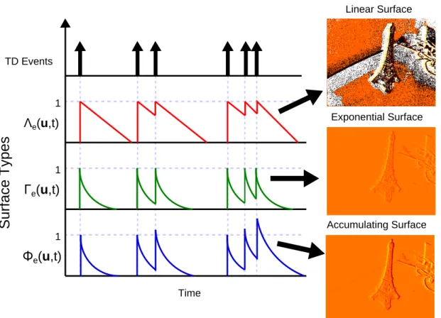
3.2 Linear, Exponential and Accumulating Surfaces of Time.

Illustration of the updates for a single pixel on the linear surface Λe (top), the exponentially-decaying surface Γe (middle) and the

accumulating exponential time surface Φe (bottom). . . 34

3.3 Exponential Time surfaces generated at five different

spa-tial resolutions. Five different surfaces of varying scales are shown. These were generated by calculating the accumulating time surface described in equation (3.6) and making use of the scale mapping in equation (3.7) with five different σ values as shown in the above figure. The five surfaces are all updated in an event-based fashion for each incoming event. . . 35

(10)

List of Figures

3.4 The effect of transformations and noise on the normalised,

sorted and orientation descriptors applied to event-based data. Three different descriptors are shown for four different fea-tures. The first row shows the original feature and their resulting descriptors for each method. The second row shows the results for a rotated version of the initial feature, with descriptor from the original feature shown as a dotted line. The third line shows the initial feature corrupted by noise and the fourth shows a completely different feature. . . 40

3.5 Diagram showing how the spatio-temporal image of time

is created for the 1D case. The ordered list of spike events is re-trieved from the camera (a), which in the case of the ATIS device, contains an additional y-dimension. The relative time difference in the spike times from the most recent event to the surrounding events defines the image of time for the arriving event (b). These relative spike timings are then stored (c) and are used to calculate the temporal orientations about the event. Only the vertical di-mension is shown in this diagram for the sake of clarity, but when performed on data from the ATIS camera, horizontal and vertical orientations are considered, yielding a full matrix of values, rather than a single vector. This is shown in (c) as the greyed boxes. . . 42

3.6 Diagram showing the differences between the arithmetic

and circular means for three angles 15◦, 45◦ and 315◦. The diagram presented highlights the difficulty in applying conventional statistical measures to circular data. Although the calculation of the arithmetic mean shown in (a) is valid, it is heavily biased by the choice of a zero reference and conventions and rotation in the data. The resulting value does not capture the true mean direction represented by the angles. A common solution to this project is to project the angles onto a unit circle and take the mean angle of the resulting vectors as shown in (b). This value better represents the concept of a mean direction for circular data. . . 45

(11)

List of Figures

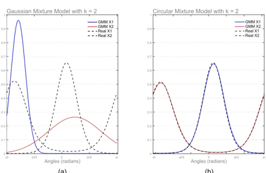
3.7 Comparison of the fits provided by a Gaussian Mixture

Model and a Circular Mixture Model for a bimodal set of orientations (k = 2). (a) The result of applying a standard Gaussian Mixture Model to circular data showing how the GMM is unable to handle the circular distribution. The two underlying distributions used to create the data are shown using the black dotted lines, and the distributions identified through the GMM algorithm are shown in red and blue. The GMM failed to con-verge and was terminated after 1000 iterations. (b) The results of the Circular Mixture Model applied to the same data. The algo-rithm converged after 61 iterations and successfully identified the underlying distributions. . . 49

3.8 Diagram showing how noise filtering is performed using

circular statistics. When a noise spike occurs in region in which no events have occurred recently (a), it generates strong temporal orientations in all directions around the event (b). When a his-togram is constructed from these events, peaks form at the cardinal and inter-cardinal directions (c). These orientations are uniformly distributed around a circle (d), and therefore can be rejected using a test for uniformity. . . 51

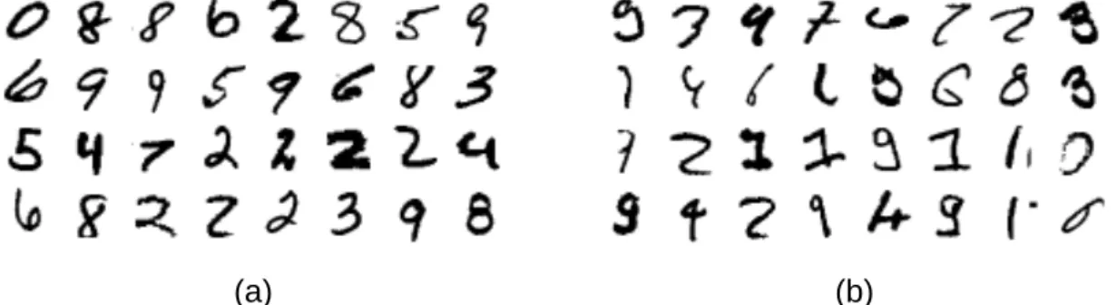
4.1 Examples of the digits in the MNIST Dataset. (a) An

exam-ple of the digits within the MNIST dataset showing 40 randomly selected digits from the training set. (b) The 40 most commonly miscategorised errors from the testing set. . . 57

4.2 Examples of some object images from the Caltech101 dataset.

The Caltech101 dataset contains 101 different object classes, with each class having a variable number of images. In addition, the images are of varying sizes. The five images presented here show an example of the variety in pose, aspect ratio and framing found in the Caltech101 dataset. . . 58

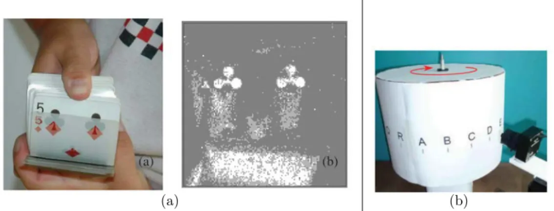
4.3 Examples of the configurations used to generate

Neuro-morphic Datasets. (a) Flicking through a deck of cards to gen-erate the pips dataset [5]. (b) An example of the data captured from the DVS sensor. (c) The rotating barrel with letters and dig-its used to generate the 36 character recognition dataset used by Orchard et al. [6] . . . 59

4.4 The configuration used to capture the MNIST and

N-Caltech101 datasets. (a) The ATIS camera mounted on a custom-built Pan/Tilt mount. (b) A top-down view of the configuration showing the relative placement of the camera and the monitor. . . 61

(12)

List of Figures

4.5 Diagram showing the three saccade-inspired motions across

each digit used in creating the spiking neuromorphic datasets. Each MNIST digit was sized so that it occupies a 28 × 28 pixel re-gion on the ATIS sensor, and three saccade motions starting in the top-left and moving in triangular motion across each digit. Due to the motion, the resulting digits sequences span a 34 × 34 pixel re-gion to ensure that the full digit remains in view during the entire saccade motion. . . 62

4.6 Overview of the classification system used for the N-MNIST

classification task. The classification system presented retriev-ing trainretriev-ing and testretriev-ing samples from the dataset and encodes them into a spatio-temporal pattern for use in the SKIM network. The process for encoding the AER data into a spatiotemporal pattern is described in Section 4.4.1. The label for the dataset is also en-coded using the training methods described in Section 4.4.5. The SKIM network produces a spatio-temporal pattern as an output, which is used either for output determination during recall opera-tions or is compared to the training signal and used to update the SKIM network during training. . . 65

4.7 Timing and Event Raster for a Digit 0 from the NMNIST

Dataset. Each sequence in the training and testing set contains three equal duration saccades. The plots shown are frame rendered by accumulating events over a period of 5ms. . . 67

4.8 Training accuracy over the first 10,000 training samples

for N-MNIST using SKIM for increasing numbers of hid-den layer neurons. Each configuration of hidhid-den layer neurons was trained sequentially through a randomly shuffled training se-quence, and tested against the testing dataset at increments of 1000 training samples. Each test was performed independently of the training, and no learning took place during the testing phase. Also shown on the graph are the accuracies due to chance and the accuracy based solely on mean number of events. The final re-sults shown on the right represent the full training accuracy tested against the full 10,000 training samples whilst intermediate points on the curve were calculated over a randomly drawn subset of 2000 testing samples. . . 70

(13)

List of Figures

4.9 Accuracy of MNIST and N-MNIST as a function of

Hid-den Layer Size. Both MNIST and the N-MNIST datasets were trained and tested using an increasing number of hidden layer neu-rons. An ELM classifier was used to learn the MNIST dataset, whilst SKIM was used to learn the N-MNIST saccades. The same training and testing order was preserved, and the results plotted were the results of testing against the entire testing dataset. Both results show the actual test results, a fitted exponential approxi-mation and the 95% confidence interval. . . 72 4.10 Histograms of the distribution of errors and their CDFs

for the Gaussian and Exponential training patterns. The results were calculated over 51 independent trials of each network. A comparison to the CDF of a Standard Normal distribution is included, and the p-value for a one-sample Kolmogorov-Smirnov test provided, demonstrating that both distributions are normally distributed. . . 74 4.11 Diagram showing the four output determination methods

evaluated for use in multi-class SKIM problems. (a) An ex-ample SKIM network with two simultaneously trained output neu-rons coding for two classes; A and B. (b) Example outputs from the two output neurons during the period in which the training spike occurs. In this example, the training utilised is the Gaus-sian training spike shown in (c). Diagrams showing the manner of calculating the four output selection methods are presented in (d), and include a label showing the theoretical winning class in each case. Note that for the Weighted Sum and Weighted Area methods, the training spike is also shown. . . 76 4.12 Comparison of the effects of the four different output

determination methods on classification accuracy with a Gaussian training pattern. The figure shows the distribution of classification accuracies over 61 trials of a SKIM network with 1000 hidden layer neurons. Each network made use of the same random training order and hidden layer configuration, with only the random weights varying from trial to trial. The network made use of a Gaussian training pattern. . . 78

(14)

List of Figures

4.13 Diagram showing different training patterns used to train the SKIM network. The three training patterns described and tested in Section 4.4.5 are shown in this figure. The Flat Output pattern represents the logical extension of a single output spike and includes two sharp discontinuities on each end. The Gaussian pattern represents the opposite approach and contains a smooth curve with no discontinuities and peaks in the centre of the pat-tern. The Exponential pattern represents a combination of the two approaches, and contains an initial discontinuity followed by a smooth and gradual decrease. . . 79 4.14 Classification error when using different training patterns

and output determination methods. Sixty trials for each pat-tern were conducted and the mean training accuracy shown in terms of percentage correctly identified. It is immediately clear from the figure that the Gaussian training pattern produces the lowest classification accuracy across all output determination meth-ods. The Flat pattern produces the best results for all methods with the exception of the Max determination method. In that case, the Exponential pattern produced the best results. . . 80 4.15 Histograms of accuracies showing the comparison between

the Gaussian and Exponential training patterns under the Max and Area determination methods. The figure shows the histograms of accuracies obtained when using the Exponential and Gaussian patterns under the Max and Area output determination methods. It serves to demonstrate the important link between training method and output determination method. It is clear that the Exponential training method is a better choice when us-ing the Max output determination method. This is of particular importance as the Max output determination method represents the easiest method to implement in hardware. . . 81 4.16 Example of a sequence from the Airplanes object

cate-gory in the N-Caltech101 dataset. The above images rep-resent frames created by accumulating the events captured over 10 ms time periods. Black pixels represent ON events generated by the ATIS sensor and white pixels indicate OFF events. Grey regions indicate that no events were received. . . 85

(15)

List of Figures

4.17 Illustration of the two methods for performing automated binary classification using SKIM without the need for ex-plicit thresholding. The two methods show how the binary prob-lem can be recast as a two-class probprob-lem. Two methods are pre-sented, which cater for different types of problems. Method 1 deals with cases where there are features in both conditions of the binary problem, and Method 2 handles the case where the one condition does not necessarily contain any separable information. . . 90 4.18 Results and confusion matrices for the 5-way

classifica-tion performed using SKIM networks of 1000 and 5000 hidden layer neurons. The confusion matrices for the 5-way N-Caltech101 classification task demonstrate the effect of hidden layer size on classification accuracy. It is important to note that the inclusion of the background class can cause instability in the SKIM network due to the lack of consistent features, and was only included to allow for comparison with the kNN classifiers explored in the Appendices. . . 94 4.19 Classification results and confusion matrices for the

4-way classification problem with SKIM. The confusion ma-trices presented here show the effect of the hidden layer size on the 4-way classification task. In this case, the background class was re-moved, resulting in an increase in classification accuracy. Although the number of classes decreased, the classification accuracy of the 1000 hidden layer neuron configuration in the 4-way task exceeded the 50.87% accuracy achieved using 5000 hidden layer neurons in the 5-way task. . . 95 4.20 Comparison per class of the results from the 4-way and the

5-way classification problems. This comparison demonstrates how the inclusion of an additional class can impact the accuracy of a classification network. Although the 4-way classification task is a subset of the 5-way classification task, it is clear from the above figure that the 4-class classification system produces superior classification results in three out of the four classes. The same number of training samples was used per category to generate these results (57 samples). . . 96 4.21 Confusion matrix for the 101-way object classification task

using SKIM with 10000 hidden layer neurons. The network achieved an accuracy of 11.14% accuracy, and trained with 15 ran-domly selected samples from each category. . . 98

(16)

List of Figures

4.22 Illustration of the encoding of intensity to delays used in creating the SpikingMNIST dataset. Each pixel in the image is assigned to a separate input channel and the intensity encoded using the mechanism illustrated above. For each pixel, a spike is placed in its respective channel at a time proportional to the grey-scale intensity of the pixel. Thus, the darker the pixel, the later in the channel the spike will occur. As the input images in the MNIST dataset use a single unsigned byte to encode intensity, the pattern length is limited to 255 time-steps. . . 100 4.23 Diagram of the structure and function of the AER-based

downsampling filters Both downsampling filters represent AER transformations and operate on AER data and produce output in the AER format. The spatial downsampling filter reduces the spa-tial resolution of the input data by a fixed downsampling factor, resulting in an output stream that maintains the temporal resolu-tion of the input. The temporal downsampling filter reduces the temporal resolution of the input stream, leaving the spatial reso-lution unchanged. These filters can be cascaded to provide both spatial and temporal downsampling. . . 103 4.24 Classification results from extended temporal

downsam-pling on the N-Caltech101 dataset. The results presented in Table 4.14 present temporal downsampling results up to 20 ms time-steps. This figure shows the classification accuracy as the time-steps are increased up to 250 ms. The accuracy peaks with a time-step resolution between 25 ms and 30 ms, achieving accu-racies up to 18.25%. Due to the length of time taken to perform each test, only a single trial of each experiment could be performed.111

5.1 Diagram of the filtering chain used for classifying directly

on the orientation outputs using SKIM. The diagram shows the steps performed for each event received from the camera, unless discarded by the noise filtering step after which the processing for that event will cease. It is important to note the polarity splitter, which allows the ON and OFF events to be handled separately. Orientations are extracted from the data for each polarity and then combined into a single AER stream. Temporal downsampling is applied to the AER data prior to conversion to a spatio-temporal pattern for the SKIM network. . . 116

(17)

List of Figures

5.2 Violin plot of the 4-way classification task on the N-Caltech101

dataset using orientation features and SKIM for varying hidden layer sizes. Twelve trials of each hidden layer size were performed, and display the large variability in the results. As this is a 4-way classification task, the accuracy due to chance is 25%. . 118

5.3 Violin plot of the classification accuracies for networks of

varying hidden layer sizes trained and tested against five categories of the N-Caltech101 dataset (airplanes, cars, faces, motorbikes and the background class). The violin plot shows the distribution of accuracies for each hidden layer size (containing 30 trials of each). Crosses indicate the mean accuracy and the green square indicates the median value. . . 121

varying hidden layer sizes trained and tested against the full 101 categories in the N-Caltech101 dataset. The violin plot shows the distribution of accuracies for each hidden layer size (containing 30 trials of each). Crosses indicate the mean accuracy and the green square indicates the median value. . . 122

varying hidden layer sizes trained and tested against the N-MNIST dataset with 10 output categories. The violin plot shows the distribution of accuracies for each hidden layer size (containing 30 trials of each). Crosses indicate the mean accuracy and the green square indicates the median value. . . 125

5.6 Effect of number of training samples on classification

accu-racy for the N-MNIST dataset. Ten trials of each experiment were conducted at 50 sample increments, and are shown as dots. The mean accuracy for each level is shown as the solid line. . . . 126

5.7 Comparison of accuracies between the SKIM and ELM

ap-proach to using orientations as features on the N-Caltech101 dataset for varying hidden layer sizes. The result presented here show the mean accuracy as a percentage of digits classified correctly. The graph also shows the standard deviations for both network types as error bars. The graph shows the increased accu-racy obtained with the ELM solution, and the lower variability it possesses over the SKIM network. . . 128

(18)

List of Figures

5.8 Structure of the time surfaces feature classification system

with online learning. The classification system for the time surface feature detector also makes use of a polarity splitter to handle the ON and OFF events separately. Time-surface features are then extracted from the incoming AER stream and sent to the adaptive threshold clustering algorithm, which identifies and learns features in an unsupervised manner. The output of the clustering algorithm represents AER events in feature space and are then used for classification. . . 130

5.9 Diagram showing the adaptive threshold clustering in a

2D space. The diagram above shows a simplified case of the adaptive threshold clustering applied to features consisting of two dimensions. An existing configuration with two normalised clus-ters is shown in (a) on the unit circle, and with independently configured thresholds. If the next feature to arrive falls within the threshold distance of an existing cluster, as shown in (b), then it is said to have matched and is assigned to the that cluster. The threshold for that cluster is then reduced as shown in (c). If the event does not match any existing clusters, as in (e), the feature is discarded and the thresholds for all clusters are increased as in (f). 134 5.10 5 × 5 feature clusters learnt from the MNIST dataset for

ON events (a) and OFF events (b). Each feature represents a normalised vector reshaped to match the size of the incoming fea-ture patches. The ordering of the feafea-tures conveys no significance. 136 5.11 Comparison of the ELM results with 11 × 11 feature

clus-ters and 5 × 5 feature clusclus-ters with an ELM network for increasing hidden layer sizes. The figure shows a comparison between the 200 11×11 pixel features and the 50 5×5 pixel features when used to generate feature events for an ELM classifier. Ten trials of each experiment were conducted, and a standard deviation under 0.5% was achieved for each hidden layer size. It is clear from the above graph that the 11 × 11 configuration performed better in every case. . . 138 5.12 The 5 × 5 pixel random features generated for the ON

events (a), and the OFF events (b) used to generate fea-ture events for the N-MNIST dataset. The random feafea-tures are initially generated, normalised and then fixed. The use of ran-dom features such as these allows for efficient hardware implemen-tations which do not require explicit feature learning, and can even exploit device mismatch to generate the random features. . . 139

(19)

List of Figures

5.13 Thresholds for the random features after learning on the training set of the N-MNIST dataset. These graphs show the final threshold values for the features provided in Figure 5.12 after training on the N-MNIST dataset. The adaptive thresholds determined by the algorithm differ greatly from the initialised value of 0.5 for both the ON and OFF clusters. It is these determined thresholds that produce the strong classification performance of the random clusters. . . 140 5.14 Comparison of the classification accuracy between the trained

5 × 5 features and the random 5 × 5 features. Each network contained 50 clusters, evenly split between ON and OFF clusters. Ten trials of each experiment were performed. . . 142 5.15 Comparison of the classification accuracy achieved with

the random clusters and trained clusters for varying hid-den layer sizes. The results for the two cluster configurations are presented for both the randomly generated clusters and the clusters learnt using the adaptive thresholding technique. . . 143

1 Histograms showing the number of events and the

dura-tion of the sequences for the training and testing datasets. The testing and training histograms are overlaid to illustrate the similar nature of the testing and training sets. There are 60,000 training samples, and 10,000 testing samples and the same bin-widths were used for both the training and testing data. . . 171

2 Average number of events per digit in the dataset (left),

and accuracy of classification per digit when attempting to classify using the number of events alone. The classifica-tion method determined the digit with the closest mean number of events to the current test sample. It is interesting to note that digit 0 has the largest number of events, whilst digit 1 has the fewest.172

3 Classification Results for a kNN Classifier based on

Sta-tistical Properties of the N-MNIST dataset. The resulting accuracy of the kNN classifiers with a k = 10 for 9 statistical mea-sures on the dataset. Statistically insignificant results are shown in grey. . . 174

4 Results for kNN Classifiers based on statistical properties

of the N-MNIST dataset. The classifiers were trained with k = 10, which was empirically found to produce marginally better results than any other value such that k > 4. The four categories were tested independently from each other. As this is a binary task, the probability due to chance is 50%. . . 177

(20)

List of Figures

5 Confusion matrices for the 5-category classification

prob-lem using a kNN classifier trained with statistical infor-mation. For each of the eleven statistical classifiers, the full 5-way confusion matrix is presented, along with the overall accuracy achieved. The matrices are coloured to highlight the distribution of classification results. . . 179

6 Classification accuracy and confusion matrices for the

101-way classification tasks performed using the kNN classi-fier. The confusion matrices for all 101 classes are shown with the colours indicating the relative number of samples falling into that classification. In the case of the 101-way classification task, the accuracy due to chance is less than 1%. These graphs show that the statistical classifiers perform poorly and favour only a small subset of the available classes. The graphs also lack the large val-ues on the diagonal corresponding to correct predictions which are present in later classifiers. . . 181

7 Comparison of the Training and Testing Times of an ELM

Classification of the MNIST digits with and without GPU Acceleration: The clear speed improvement in training times resulting from the GPU optimisation is shown in (a), whereas (b) shows the more moderate improvements in testing time when using the GPU acceleration. The graph in (b) shows how the overhead from the GPU memory transfers negatively affect the testing times for lower numbers of hidden layer neurons. . . 186

8 Effect of Differing Levels of Floating Point Precision on

Accuracy and Training Time For GPU Optimisation. The training times (a) and testing times (b) for the same GPU optimi-sations running at single and double precision, showing that using single precision yields a significant speed advantage. The accuracy in terms of incorrect digits when classifying against the MNIST dataset is shown in (c), and demonstrates that there is no loss of accuracy associated with the lower float point precision. . . 187

9 Comparison between the GPU SKIM implementation and

the Normal SKIM Implementations for varying hidden layer sizes. The training time to train all ten trials is shown in (a) and shows a dramatic improvement for the GPU implemen-tation. The average across time for all ten trials is shown in (b) and represents just the training time itself without any overhead. It is clear from both plots that the GPU implementation greatly outperforms the standard implementation. . . 189

(21)

List of Figures

10 Illustration of the under-determined and over-determined

region of an LSHDI network of 1000 hidden layer neurons and the performance characteristic for an MNIST

classi-fier trained on varying numbers of training samples. . . . 190

11 Effect of initial output weights on classifier performance

on the MNIST dataset with iterative training. The graph shows the results of training an iteratively trained network with 1000 hidden layer neurons on varying number of training inputs from the MNIST dataset using both randomly initialised output weights and output weights initialised to zero. Note that these results show the mean accuracy achieved over 10 trials of each number of training samples. . . 192

12 The 100 ON Clusters for the N-MNIST dataset for 11 × 11

pixel features generated by the Adaptive Threshold Clus-tering. The resulting 100 feature clusters after training on all 60,000 training digits in the N-MNIST dataset. The order conveys no particular significance. . . 196

13 The 100 OFF Clusters for the N-MNIST dataset for 11×11

pixel features generated by the Adaptive Threshold Clus-tering. The resulting 100 feature clusters after training on all 60,000 training digits in the N-MNIST dataset. The order conveys no particular significance. . . 197

14 The 100 random ON Clusters for the N-MNIST dataset

for 11 × 11 pixel clusters. These feature clusters are normalised, and the adaptive thresholding technique was used to determine the individual thresholds for each cluster. . . 198

15 The 100 random OFF Clusters for the N-MNIST dataset

for 11 × 11 pixel clusters. These feature clusters are normalised, and the adaptive thresholding technique was used to determine the individual thresholds for each cluster. . . 199

(22)

Nomenclature

Greek Symbols

β Linear Output Weights

θk The inverse of the correlation matrix

wi,j Inputer layer weights

Acronyms

AER Address-Event Representation

AIT Austrian Institute of Technology

ATIS Asynchronous Time-based Imaging Sensor

BRIEF Binary Robust Independent Elementary Features DAVIS Dynamic and Active-Pixel Vision Sensor

DoG Difference of Gaussians DVS Dynamic Vision Sensor ELM Extreme Learning Machine

EM Exposure Measurement

FPGA Field Gate Programmable Array GMM Gaussian Mixture Models

HOG Histogram of Oriented Gradients

LSHDI Linear Solutions to Higher Dimensional Interlayers NEF Neural Engineering Framework

(23)

Nomenclature

OPIUM Online Pseudoinverse Update Method PCA Principle Component Analysis

QVGA Quarter Video Graphics Array SIFT Scale-Invariant Feature Transform SKIM Synaptic Kernel Inverse Method SURF Speeded-up Robust Features

(24)

Executive Summary

The importance of computer vision in modern technology is continuously increas-ing, both in terms of usage and the demands placed upon it. The field is also ex-periencing unprecedented levels of interest and growth, spurred on by large-scale investment in future technologies such as self-driving vehicles, autonomous drones and household robotics. The underlying technologies and hardware requirements for these applications have also experienced rapid growth, often eclipsing the ca-pabilities of current state-of-the-art algorithms and processing techniques. The tasks in computer vision are inherently difficult and challenging problems, and despite the advances in computational power, pixel resolution, and frame rates, even the most sophisticated methods fall far short of the robustness, reliability and energy consumption of biological vision systems.

Silicon retinas, such as the Dynamic Vision Sensor (DVS) and the Asyn-chronous Time-based Imaging Sensor (ATIS), attempt to replicate some of the benefits of biological retinas and provide a vastly different paradigm in which to sense and process the visual world. Tasks such as tracking and object recognition still require the identification and matching of local visual features, but the de-tection, extraction and recognition of features requires a fundamentally different approach, and the methods that are commonly applied to conventional imaging are not directly applicable.

The work in this thesis explores methods to detect features in the spatio-temporal information produced by event-based vision sensors and then utilises these features to perform recognition and classification tasks. This work explores the nature of detecting features in event-based data and presents two feature detection methods inspired by concepts and methodologies employed by highly successful conventional computer vision algorithms such as the Scale Invariant Feature Transform (SIFT) and Histograms of Gradients (HOG).

The first feature detector makes use of spatio-temporal gradients to extract features from the event-stream. Applying circular statistics to the orientation data allows for efficient noise removal and feature detection using mixtures models of circular distributions.

(25)

Executive Summary

incoming event-based visual data. Feature extraction makes use of a modified and event-based corner detection approach to identify features of interest, and the use of descriptors allows for invariance to specific affine transformations.

This thesis introduces two new neuromorphic datasets, MNIST and N-Caltech101, created from existing and well-established computer vision datasets and intended to address the lack of consistent and well-adopted benchmarks in the neuromorphic community. Based on the MNIST dataset and the Caltech101 datasets, these datasets maintain the structure and methodology of the originals, allowing for comparison and contrast to existing conventional computer vision systems. This thesis provides a thorough analysis of these two datasets and includes benchmarks based on statistical classifiers as a baseline for classifier performance.

The Online PseudoInverse Update Method (OPIUM) and the Synaptic Kernel Inverse Method (SKIM) form the basis of the learning systems used in this work, and the results achieved validate their use in both event-based vision systems and on large neuromorphic datasets.

Additionally, this work makes use of SKIM networks applied to the largest datasets to date, implementing the largest hidden layer sizes and simultaneously training the largest number of output neurons. The success of the classifiers built using these SKIM networks validates both the underlying SKIM algorithm and its applicability to event-based tasks such as those presented in this work. The further work on optimisation of the SKIM network for parallel GPU implemen-tation serves as a first-step toward the faster hardware-based implemenimplemen-tations required for real-time operation of such systems.

The work in this thesis deals with the classification of objects from the event-based output of a silicon retina and explores two approaches to performing such classification; one operating on the event-streams directly, and the other making use of extracted features from the event-based data.

Exploring the nature of performing classification on event-based data directly, this work characterises the performance of these systems and achieved accuracies up to 92.87% on the N-MNIST dataset and 11.14% on the N-Caltech101 dataset. A study into training patterns and output determination methods is also pre-sented, along with means and methods for handling non-uniform image sizes.

This thesis also investigates the effects of both spatial and temporal down-sampling on event-based vision data, and found that it produces improved clas-sification accuracy. For a given network containing 1000 hidden layer neurons, the spatially downsampled systems achieved a best-case accuracy of 89.38% on N-MNIST as opposed to 81.03% with no downsampling at the same hidden layer size. On the N-Caltech101 dataset, the downsampled system achieved a best case accuracy of 18.25%, compared to 7.43% achieved with no downsampling.

(26)

Executive Summary

layer to the network, which converts the input from a 2D space defined by the silicon retina, to a feature space defined by the feature detectors. These clas-sification networks address a number of issues relating to network size and the handling of non-uniform image sizes, and produced the best classification results on the N-MNIST dataset, achieving 91.6% ± 1.69% with orientation features and an ELM network, and 94.71% ± 0.36% with the time surface features and a SKIM network.

Given the performances of the classification systems presented, this work serves to validate the two neuromorphic datasets introduced and provides a range of benchmark accuracies for them. The results also demonstrate the viability of event-based object classification and proves that it can be accomplished in an based manner. The work also validates the applicability of SKIM to event-based data, and specifically its applicability to classification on event-event-based vision data.

Finally, the improved results achieved using the feature detectors and the downsampling indicate the importance of both the temporal and spatial informa-tion in the event-streams from a silicon retina, and serve to further demonstrate the benefits to using such devices.

(27)

Chapter 1 Introduction

1.1 Motivation

Computer vision is becoming an increasingly important and active field of study and technologies arising from its applications are finding widespread adoption in both consumer and industrial products which require sophisticated visual systems in order to safely and successfully interact with the world around them.

One of the fundamental tasks underlying much of computer vision is the de-tection, tracking and recognition of visual features. It is an inherently difficult and challenging problem, and despite the advances in computational power, pixel resolution, and frame rates, even the state-of-the-art methods fall far short of the robustness, reliability and energy consumption of biological vision systems.

Silicon retinas, such as the Dynamic Vision Sensor (DVS) and the Asyn-chronous Time-based Imaging Sensor (ATIS), attempt to replicate some of the benefits of biological retinas and provide a vastly different paradigm in which to sense and process the visual world. Tasks such as tracking and object recognition still require the identification and matching of local visual features, but the de-tection, extraction and recognition of features requires a fundamentally different approach, and the methods that are commonly applied to conventional imaging are not directly applicable.

As a result, there exists a need for the development of new algorithms and paradigms in which to handle and process event-based image data. These al-gorithms and systems also require characterisation and comparison to existing approaches to visual sensing using conventional cameras in order to verify the in-formation encoded into the spatio-temporal inin-formation produced by these event-based devices.

(28)

1. Introduction

1.2 Aims

This thesis seeks to explore methods to detect features in the spatio-temporal information from event-based vision sensors, and then to utilise these features to perform recognition and classification tasks.

This work will explore the nature of detecting features in event-based data, and present methods to determine and detect features in manner that preserves

the event-based nature of the data. Making use of concepts often employed

in conventional computer vision, this work investigates the adaption of these methods to an event-based paradigm.

A framework for detecting, recognising and classifying features will be devel-oped to showcase and demonstrate the efficacy and efficiency of these detectors and to validate their performance using both real-world and simulated data. Ad-ditionally, two new spiking neuromorphic datasets, based on existing computer vision datasets, will be introduced and characterised to allow for comparisons to conventional computer vision systems.

1.3 Main Contributions of this Work

The main contributions of this thesis are the development of novel feature detec-tion, classification and recognition algorithms for event-based visual tasks. These algorithms and systems operate in an event-based manner, and perform learning and computation in a similar fashion where possible.

Each section in this thesis contains a detailed discussion of the specific con-tributions made.

1.4 Relevant Publications

Parts of this work have already been published, or are currently under review. A list of these works can be found below:

• Synthesis of neural networks for spatio-temporal spike pattern recognition and processing

J. Tapson, G. Cohen, S. Afshar, K. Stiefel, Y. Buskila, R. Wang, T. Hamil-ton, and A. van Schaik

Frontiers in Neuroscience, vol. 7, 2013.

I assisted in the development of the SKIM algorithm, contributing to the writing, the testing and in the production of the results for the paper.

(29)

1. Introduction

• ELM solutions for event-based systems J. Tapson, G. Cohen, and A. van Schaik

Neurocomputing, vol. 149, pp. 435-442, Feb. 2015.

I produced results for the paper and wrote the implementation of the algo-rithms used.

• Converting Static Image Datasets to Spiking Neuromorphic Datasets Using Saccades

G. Orchard, A. Jayawant, G. Cohen, and N. Thakor, arXiv preprint arXiv:1507.07629 (2015).

I produced the statistics and the classification results for the all the methods in the paper (with the exception of the HFirst results).

• Learning Motion Selective Receptive Fields In Spiking Neurons G. Orchard, G. Cohen, N. Thakor, and J. Tapson

IEEE Transactions on Neural Networks and Learning Systems (under re-view)

I implemented and produced the results for the SKIM networks used in this paper

• A Memristor-based Hardware Implementation of Synaptic Ker-nels for Dendritic Computation

J. Burger, G. Cohen, C. Teuscher, and J. Tapson ELM2014 Conference, Singapore.

I contributed the SKIM portion of this paper and integrated the memrister models into it.

1.5 Structure of this Thesis

This thesis is structured as follows:

• Chapter 2 presents a detailed literature review covering feature detection in conventional computer vision, the classification systems used in this thesis, and the silicon retina devices used in this work.

• Chapter 3 introduces two feature detectors for use with event-based visual data.

(30)

1. Introduction

• Chapter 4 explores object recognition and classification using event-based visual data, and showcases two datasets created specifically for benchmark-ing neuromorphic spike-based systems.

• Chapter 5 extends the object recognition framework introduced in Chapter 3 through the use of the feature detectors to convert the classification task from a 2D spatial classification task to one in a feature-space.

• Chapter 6 provides the conclusions to the work performed in this thesis, and includes a discussion of potential future work.

Appendix A contains a detailed statistical analysis of the MNIST and N-Caltech101 datasets. Appendix B describes the optimisation techniques used for the classification systems in this thesis, which allowed for the depth and breadth of the experiments conducted. Appendix C presented additional figures and tables included as supplementary material.

(31)

Chapter 2 Literature Review

2.1 Introduction to Computer Vision

The field of computer vision is currently experiencing an unprecedented level of interest and growth, spurred on by large-scale investments in future technologies such as self-driving vehicles, autonomous drones, household robotics, and even the prolific growth of mobile phones and the cameras within them. The under-lying technologies and hardware requirements for these applications have also experienced rapid growth, and have often eclipsed the capabilities of the current state-of-the-art algorithms and processing techniques. Computer vision therefore lies at the crux of a large swath of future technologies, and has the potential to offer solutions to these problems. It is a field made additionally complicated by the dramatic range of applicable contexts and platforms, ranging from low-power mobile devices, to high-precision and life-critical robotic surgery techniques.

One of the fundamental tasks underlying much of computer vision is the de-tection and tracking of visual features. It is inherently a difficult and challenging problem, and despite the advances in computational power, pixel resolution, and frame rates, even the state-of-the-art methods fall far short of the robustness, reliability and energy consumption of biological vision systems.

At the heart of any visual system lies a device that captures information from the 3D scene and encodes it into a representation fit for further processing, and from which further actions can be taken. In the majority of cases in computer vision, this device is a camera that creates a 2D representation of a 3D scene. It is this transformation, and the loss of information that arises from it, that causes much of the difficulty in visual feature detection and tracking. Other features that complicate the problem include noise, motion (both of objects in the scene and the camera itself), occlusions and illumination changes. The ability to exhibit the appropriate degree of invariance to these issues is a core requirement of both a feature detection system, and a feature tracking system.

(32)

2. Literature Review

The majority of the research into computer vision focuses on using a single camera. Multiple cameras can alleviate some of the issues regarding camera pose and viewpoint issues, but there are also new classes of imaging devices emerging that make use of other methods to create representations of the world around them. These include depth sensors, infrared sensors, and a class of biologically-inspired neuromorphic vision devices often referred to as Dynamic Vision Sensors (DVS).

This review chapter serves to provide the background and context for the work presented in the following chapters. It begins with a discussion of the field of neuromorphic imaging devices which generate event-based visual data and describes the nature of these devices and the means used to represent output data. Finally, the section provides a detailed description of the specific device used in this thesis.

The work in this thesis draws heavily on the existing body of knowledge encompassing the field of computer vision for conventional imaging devices. The field of feature detection on images is well-established and has produced a number of algorithms and techniques that enjoy widespread use, both in research and industry. The second part of this literature review provides a summary of the field of feature detection in computer vision and highlights the important algorithms which form the basis for much of the work in this thesis.

The learning and recognition of features is an important task, and an area in which this work makes a large contribution. The last section of this litera-ture review introduces a class of learning algorithms which form the basis of the recognition systems presented in this work.

2.2 Neuromorphic Imaging Devices

The process by which information is processed in neuro-biological systems is vastly different from the mechanisms used by modern computers and devices. Whereas computers use high-speed clock rates, synchronous logic and precisely matched hardware, neuro-biological systems make use of slow signals, inhomo-geneous components and make use of noise as a feature in their design. These biological systems outperform even the most sophisticated hardware at a myriad of real-world tasks, whilst consuming only a fraction of the power.

Conventional cameras output visual information in the form of frames at a constant rate. These frames include highly redundant information, as every pixel produces a value for every frame at a fixed frame rate and global exposure time for all pixels. Biological retinas, by contrast, exhibit a far more efficient encoding mechanism, and transmit only relevant information in an asynchronous manner, which leads to far greater information encoding and much lower energy

(33)

require-2. Literature Review

ments [7].

2.2.1 Neuromorphic Engineering

Neuromorphic engineering is the term given to the study and development of electronic systems that attempt to replicate and mimic the structure, function and organisation of these neuro-biological systems. Electronic implementations of neural circuits began with the construction of perceptrons in 1958 [8], but it was the combination of the rise of Very Large-Scale Integration (VLSI) and a focus on utilising the non-linear characteristics of transistors that lead to development of the concept of neuromorphic engineering by Carver Mead [9].

Recently, the term neuromorphic has come to refer to a wider range of systems that attempt to model the behaviour of neural systems in analogue, digital and mixed-signal systems [10]. The most successful of these systems have focused on emulating a single sensory transduction, for such senses as vision, sound and tactile information. These include the development of silicon cochleas, visual motion sensors and silicon retinas. It is the latter that forms the basis of the motivation for this thesis.

2.2.2 Address Event Representation (AER)

Of paramount importance to any information processing system is the mechanism by which information is transmitted and received. This is of particular relevance in attempting to model elements of neuro-biological systems, as they boast a degree of point-to-point connectivity that is not feasible to implement directly with current technologies. Neuromorphic systems are often spike-based, and make use of a spike-based hardware technique known as Address-Event Representation (AER).

AER has become the standard neuromorphic interfacing protocol, specifically for multi-chip neuromorphic systems [11] but also in terms of intra-chip commu-nication in mixed-signal devices, and has proved to be a successful and powerful protocol for simulating large point-to-point connectivity, in which sparse events need to be communicated from multiple sources over a narrow channel [12]. A handshaking protocol allows multiple devices to share a common communication bus, and static timing between events is statistically preserved, due to the asyn-chronous nature of the event generation and the random order in which events occur [13].

Figure 2.1 shows a simple AER implementation, in which an arbiter on the transmitting device assigns a unique address to each of its neurons, and when a neuron spikes, an event is generated that contains its unique address and any additional information required. The AER protocol then transmits this spike

(34)

Device 1

N3 N2 N1 A rbi ter/ E ncod er

Digital Bus

Decoder _N3 N2 N1

Device 2

Figure 2.1: Inter-device communication using Address Event Represen-tation (AER). The neurons in Device 1 are assigned a unique address by the arbiter, and when they spike, an event is sent serially down the AER data bus that connects the two devices together. A decoder on the second device recon-structs the spike and makes it available to the target neurons. This figure has been adapted from [1].

serially over a communication bus to a receiver, which decodes the event and selects the appropriate destination. Multiplexing and arbitration only occur when the spike rate of the chip exceeds the transmission capacity of the communication link.

AER has been widely adopted for use in silicon retinas [1, 14, 15, 16, 17], neural processors [18, 19, 20, 21] and in silicon cochleas [22, 23, 24, 25, 26, 27].

2.2.3 Silicon Retinas

Although the first electronic models of the retina were developed in the 1970’s [28], it was the integrated silicon retina by Mahowald and Mead [29] that represented the first viable imaging device. This was followed by a more biologically realistic implementation from Boahen’s group in 2004 [30, 31], which performed better but suffered from large variability in pixel response. An implementation by Ruedi et al. solved a number of issues involving transistor mismatch and poor dynamic range found in previous retinas [32].

There have been a number of other silicon retinas developed. These include a number of retinas that compute and output spatial contrast [14, 33, 34], temporal intensity retinas [35], temporal difference retinas [36, 37], centre of mass detec-tors for multiple objects [38], a prototype microbolometer [39] and the motion detection system for the Logitech trackball products [40].

The two most relevant devices to this thesis are two of the most recent Tem-poral Difference (TD) devices, namely the Dynamic Vision Sensor (DVS) [41] and the Asynchronous Time-based Imaging Sensor (ATIS) [2] .

(35)

AER is a natural fit for the data arising from silicon retinas, as the address encode the physical (x, y) location of the pixel, and optionally can include some information regarding the illumination falling onto it. Inter-spike intervals and spatial relationships between spike times encode the information about the scene. In a Temporal Difference (TD) device, each pixel only outputs data in re-sponse to a change of illumination [42]. Given a static scene, these pixels will not produce any output and therefore the data-rate from the device is dependent on the activity in the scene. Each pixel emits an AER event containing the physical location of the pixel in the array, and generally a single bit of information to indicate whether the illumination on the pixel increased or decreased.

The following notation is commonly used to represent an event emitted by a TD pixel:

e = [x.y, t, p]T (2.1)

In which the event e indicates that the pixel located at u = [x, y]T _{on the}

camera sensor generated a change event in response to an illumination change at time t, with the direction of the change in illumination encoded as p ∈ [−1, 1], in which p = 1 is conventionally referred to as an ON event, representing an increase in illumination, and p = −1 correspondingly representing an OFF event in which a decrease in illumination occurred.

The output of a TD sensor represents a spatio-temporal image of the changes in illumination in a scene. The temporal resolution is limited by the rate at which events can be read from the physical hardware (usually on the order of microseconds). Unlike conventional cameras, there is no concept of frames, as the data arrives entirely asynchronously.

A second class of devices, known as Exposure Measurement (EM) devices,

measure the absolute pixel illumination intensity. Applying the same

asyn-chronous approach to these devices allows each pixel to integrate independently, which greatly improves the dynamic range of the sensor [43], as the minimum integration time is set by the transmission rate of the arbiter, and the maximum integration time is subject only to effects of noise and dark current.

The exposure measurement pixels also operate in a spike-based manner by encoding the relative illumination intensity in the inter-spike interval of two se-quential events from the same pixel. The exposure measurement circuit operates using two thresholds applied to the change of illumination on the given pixel. When triggered, the EM circuit begins integrating its photocurrent, emitting a spike when reaching the lower threshold, and a second spike when encountering the upper threshold. This results in an inter-spike time between the two events that is proportional to the illumination falling on the pixel itself.

(36)

a feature detection, tracking and recognition framework for use with spatio-temporal data derived from a TD sensor.

2.2.4 Asynchronous Time-based Imaging Device (ATIS)

The data and the datasets used in this work make use of a specific DVS sensor known as the Asynchronous Time-based Imaging Device (ATIS), which contains both a TD and EM circuit for every pixel. Other imaging devices, such as the Dynamic and Active-Pixel Vision (DAVIS) camera [44], offer similar capabilities, but were not used in this work.

The ATIS is a CMOS dynamic vision and image sensor developed by the Aus-trian Institute of Technology (AIT) and draws inspiration from the data-driven nature of biological vision systems [45]. Unlike conventional camera methodolo-gies, which rely on artificially created timing signals that are independent of the source of the visual information [41], biological retinas do not produce frames or pixel values but rather encode visual information in the form of sparse and asynchronous spiking output.

The ATIS sensor offers a QVGA resolution with a 304 × 240 array of au-tonomously operating pixels, which combine an asynchronous level-crossing de-tector (TD) and an exposure measurement circuit (EM). These pixels do not output voltages or currents, but rather encode their output in the form of asyn-chronous spikes in the address-event representation (AER) [46].

Figure 2.2 shows the structure and function of an individual pixel and nature of their asynchronous event outputs. The change detection circuit outputs events in response to a change in illumination of a certain magnitude, and is also capable of triggering the exposure measurement circuit, which then generates two events with the absolute instantaneous pixel illumination encoded as the inter-spike timing between them.

This ability to couple the TD and EM circuits results in EM readings gen-erated only in response to changes in the scene, providing a form of hardware level compression which allows for highly efficient video encoding. This is most significant in slowly-changing scenes, where the majority of the illumination on each pixel remains constant.

In addition, the combination of change events from the TD and the two spikes emanating from the exposure measurement circuitry can be combined to produce a quicker gray-scale image approximation by using the inter-spike times between the TD event and the first EM measurement [47]. This can then be later updated using the final EM spike to produce a more accurate result.

As each pixel operates autonomously, there is no need for a global exposure rate and therefore each pixel is able to optimise its integration time independently. This results in a sensor with high dynamic range and improved signal-to-noise

(37)

Change Detector

Exposure Measurement ATIS Pixel

Trigger

Log Pixel Illumination

PWM Grayscale Eventst Change Events (ON/OFF)

Gray level ≈ 1/t

Figure 2.2: Functional diagram of an ATIS pixel [2]. Each pixel in the ATIS camera contains both a change detector circuit (CD) and an exposure measure-ment circuit (EM). The CD circuitry generates events in response to a change in illumination of a certain magnitude (specified by an externally configurable threshold). The CD circuitry can also be configured to trigger the EM circuitry, which encodes the absolute light intensity on the pixel in the inter-spike interval between two spikes. Each pixel operates asynchronously, eliminating the need for a global shutter and is capable of individually encoding change events and events containing illumination information. These events are generated and transmitted asynchronously from each pixel in the sensor.

ratio. The asynchronous nature of the change detection also yields almost ideal temporal redundancy suppression and results in sparse encoding of the visual information in the scene.

The output of these cameras is a spatio-temporal pattern with the location of the pixel generating the event contributing the spatial information (u from Equation (2.1)), and the time (t) at which the pixel generated the event providing the temporal information. The temporal resolution is limited only by the speed at which the sensor can produce events (typically on the order of microseconds [2]).

It is important to note that the ATIS is characterised as supporting a maxi-mum event rate of 30 million events per second [48], yielding a theoretical time resolution of 33 ns. This value represents the smallest possible time measurable between two events and is generally not sustainable. In practise, it is not always possible to read events at the speed at which they occur, and the action of the arbiter may result in events being read in a different order to the order in which they occurred. Temporal event accuracy is generally on the order of microseconds [49], and for that reason, most ATIS hardware limits the temporal resolution to microseconds.

en fr

HAL Id: tel-01426001

https://tel.archives-ouvertes.fr/tel-01426001

Event-Based Feature Detection, Recognition and

Classification

Gregory Kevin Cohen

To cite this version:

University of Pierre et Marie Curie

Western Sydney University

Doctorate school: SMAER

Event-Based Feature Detection, Recognition and

Classification

Defended by Gregory Kevin Cohen

Discipline/Speciality

Robotic

Supervised by:

Pr. Ryad Benosman, Pr. André van Schaik and Pr. Jonathan Tapson

Defended 5

September 2016

Abstract

Acknowledgements

Contents

List of Figures

Nomenclature

Executive Summary

Chapter 1

Introduction

1.1

Motivation

1.2

Aims

1.3

Main Contributions of this Work

1.4

Relevant Publications

1.5

Structure of this Thesis

Chapter 2

Literature Review

2.1

Introduction to Computer Vision

2.2

Neuromorphic Imaging Devices

2.2.1

Neuromorphic Engineering

2.2.2

Address Event Representation (AER)

Device 1

Digital Bus

Device 2

2.2.3

Silicon Retinas

2.2.4

Asynchronous Time-based Imaging Device (ATIS)

_{September 2016}