Assessment of Regression-based Techniques for Data Location Verification at Country-Level

(1)

HAL Id: hal-02089272

https://hal.archives-ouvertes.fr/hal-02089272

Submitted on 3 Apr 2019

HAL is a multi-disciplinary open access

archive for the deposit and dissemination of

sci-entific research documents, whether they are

pub-lished or not. The documents may come from

teaching and research institutions in France or

abroad, or from public or private research centers.

L’archive ouverte pluridisciplinaire HAL, est

destinée au dépôt et à la diffusion de documents

scientifiques de niveau recherche, publiés ou non,

émanant des établissements d’enseignement et de

recherche français ou étrangers, des laboratoires

publics ou privés.

Assessment of Regression-based Techniques for Data

Location Verification at Country-Level

Malik Irain, Zoubir Mammeri, Jacques Jorda

To cite this version:

Malik Irain, Zoubir Mammeri, Jacques Jorda. Assessment of Regression-based Techniques for Data

Location Verification at Country-Level. 6th International Conference on Wireless Networks and Mobile

Communications (WINCOM 2018), Oct 2018, Marrakesh, Morocco. pp.1-7. �hal-02089272�

(2)

Any correspondence concerning this service should be sent

to the repository administrator:

tech-oatao@listes-diff.inp-toulouse.fr

This is an author’s version published in:

http://oatao.univ-toulouse.fr/22712

Official URL

DOI :

https://doi.org/10.1109/WINCOM.2018.8629684

Open Archive Toulouse Archive Ouverte

OATAO is an open access repository that collects the work of Toulouse

researchers and makes it freely available over the web where possible

To cite this version:

Irain, Malik and Mammeri, Zoubir and Jorda, Jacques

Assessment of Regression-based Techniques for Data Location Verification at

Country-Level. (2018) In: 6th International Conference on Wireless Networks

and Mobile Communications (WINCOM 2018), 16 October 2018 - 19

October 2018 (Marrakesh, Morocco).

(3)

Assessment of Regression-based Techniques for Data Location

Verification at Country-Level

(Invited Paper)

Malik Irain, Zoubir Mammeri, Jacques Jorda IRIT – University of Toulouse, France {malik.irain,zoubir.mammeri,jacques.jorda}@irit.fr

• Cloud framework-based DLV approaches [5], [15], [19]

aim at installing a software framework on CSP. Such a framework is in charge of guaranteeing data location by forbidding data moves to unauthorized locations.

• Hardware-based DLV approaches [1], [3], [14] aim at

providing a tamper-proof hardware root of trust. Such a hardware is physically connected to the CSP’s machines, thus guaranteeing its own location and the connected machines.

• Landmark-based DLV approaches [4], [6], [7], [8], [9],

[13], [17], [18] aim at providing communication-based solutions. Such solutions allow users to estimate data lo-cation using landmarks, which are hosts connected to the Internet whose physical locations are known and that can interact with the user and with the CSP. Prior to launching the DLV process, landmarks are deployed by the user, in a way such that he/she tries to surround location in which data are supposed to be located. Then, landmarks interact with each other, building a model predicting distance, generally based on the Round-Trip Times (RTTs) mea-sured during these interactions. Afterwards, when the user requests location verification, landmarks probe the CSP. Feeding CSP-related RTTs to built model of distance prediction allows to derive a geographic zone, reflecting the CSP estimated location according to the measured RTTs. Location agreed from the SLA should be included in the estimated zone, otherwise it is very likely that data were moved from the agreed location.

In the sequel, we address landmark-based DLV approaches and compare their location accuracy. For performance reasons, including data access delay and robustness, the data may be stored at different locations by the CSP and the users are aware of the distribution or duplication of their data. Without loss of generality, we assume that the entire data for which DLV is run are in a single location. Indeed, iterating the verification process described in the following sections would contribute to consider multi-location CSPs. The objective of the paper is to present results of experimentation based on a platform of data collection. DLV approaches are evaluated with the same dataset.

The rest of this paper is organized as follows. Section II presents the compared DLV approaches. In Section III, dataset collecting and preprocessing are described as well as assessment methodology. Section IV concludes the paper.

Abstract—Data storage in the Cloud became a very popular service. However, delegation of data management results in loss of control from user perspective, in particular regarding the real location where data are stored. Thus, data location verification in the Cloud is a challenging issue. Among the huge methods proposed to consider data location verification, this paper focuses on machine learning based methods, which use network Round Trip Times as main metric. In particular, it provides experimental results based on country-wide dataset collected through Grid’5000 platform. Results show the capacities of regression-based methods to support data location verification at specific accuracy depending on user requirements.

I. INTRODUCTION

Nowadays companies, administrations, and individuals let data storage be handled by large-scale distributed storage systems, called Cloud services. Thus, they are relieved of management and maintenance of equipment used for data storage. Doing so, users have to trust their Cloud Service Provider (CSP) as they lose control over their data. To make Cloud services more widely accepted users can implement requirements in QoS clauses, including clauses about data location in the Service Level Agreement (SLA). Legal issues [10], privacy [13], and performance [8] are the main reasons for data location requirements.

Limitations about data location are often enforced by gov-ernments, which require some data to be stored in certified data centers with a location clause provided in the SLA [10], [11], [16]. That is why Cloud services users need to have means to verify their data location. However, Cloud infrastructure virtualization makes location verification a challenging issue, as data location cannot easily be known, even by the CSP in some cases. Moreover, even when SLA includes an initial clause about location and the clause is initially honored, the CSP is still able to change data location by moving them to another country to cut costs, by mistake or maliciously.

When a location clause exists in the SLA, the CSP agrees on it and should store the data at the specified location. Users can either trust the CSP and there is no data location verification problem, or assume that the CSP can be malicious and store data in an inappropriate location and they have to deploy mechanisms enabling data location verification at any time. Huge approaches addressing this problem were proposed in lit-erature [12]. Three DLV (data location verification) approaches classes are commonly distinguished:

(4)

II. OVERVIEW OFDLVAPPROACHES

Most of the landmark-based DLV approaches are based on the same principle under the assumption that there is a relation-ship between RTT and distance. First, all the landmarks whose positions are known interact with each other, sending requests to each other and measure the RTTs of requests-responses. Hop count may also be collected. Using measurements, a ma-chine learning model is built to estimate the distance according to measurements. After training phase, learning model can be evaluated by making measurements between landmarks and CSP to infer CSP location. Multilateration is used to calculate the zone of intersection where data is expected to be stored. In the sequel, N denotes the number of measures used in training and ri

l,k and dil,k the ith training RTT measure from

landmark l to another landmark k and the associated distance, respectively. The distinctive feature between DLV approaches is the distance model they use. A distance is associated to RTT value. Among the proposed DLV approaches, we select three, which are representative in the field of data location verification [12].

A. Bestline-based approach

Distance models used in Fotouhi et al. [8] and Gondre and Peterson [9] approaches are based on bestline. The latter is the highest linear function lower than all points in the Distance-RTT graph. Bestline-based model results in distance overestimate; depending on the dataset coverage, the returned area should include the real location. Each landmark builds its own function to describe the bestline, which represents distance in function of RTT, as follows:

\

d _best_l= a bestl× r + b bestl

where variable r is associated with RTT value; slope aland

intercept bl of l landmark’s bestline are calculated according

to bestline definition.

B. Linear regression-based approach

Watson et al. [18] and Benson et al. [4] used a linear func-tion obtained through linear regression as distance model. The slope aland intercept bl, associated with any landmark l, are

computed using linear regression. Consequently, inaccuracy in the result grows according to the spread of RTT values for a given distance.

\ d _linreg

l= a linregl× r + b linregl

C. Polynomial regression-based approach

Eskandari et al. [7] proposed to use a polynomial function to estimate the distance in function of RTT. It should be noticed that, in Eskandari’s approach, all landmarks use the same coefficients. Assuming M is the degree of the polynomial function, distance estimation model is:

\ d _{polyreg =} M X j=1 a _polyreg_j_{× r}j + b polyreg

a_j _{coefficients and b are obtained through polynomial} regression. As mentioned for previous approach, when regres-sion is used, uncertainty in the result grows according to the spread of RTTs for a given distance. In machine learning practice, degree M is selected depending on the shape of measurements. In our experimentation, polynomial degree is increased until no improvement in results is observed.

III. METHODOLOGY AND EXPERIMENTATION SETUP

A. Dataset collection

Authors of DLV approaches provided some simulation or experimentation results, which were obtained through specific real or simulated environments and hypotheses, to empha-size the performance of their approaches. Unfortunately, the diversity of simulation/experimentation environments makes comparison between results either infeasible or unfair. Our first contribution is to design and implement a distributed framework to collect credible and representative dataset at country level, France in our work. Then, the same data is used to evaluate all three DLV approaches we selected. Our data collection was run over a long period (in month), while many authors evaluate their solutions using data collected online during a short period of simulation (in second).

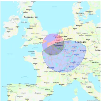
Fig. 1: Grid’5000 Map and nodes connection To collect the dataset, we used Grid’5000 platform [2]. The latter is a french distributed infrastructure composed of nodes located at main french cities including Grenoble, Lille, Lyon, Nancy, Nantes, Rennes, and Sophia and one site in Luxembourg. Grid’5000 nodes are connected through 10 Gigabits dedicated links as shown on Figure 1.

On each node, a script was activated to send requests to all the other nodes each 5 minutes from May 22nd _{2018 to June}

22nd _{2018. We collected a total of 614,244 samples between}

all Grid’5000 nodes. A sample consists of a timestamp, an RTT, and a hop count obtained with traceroute command.

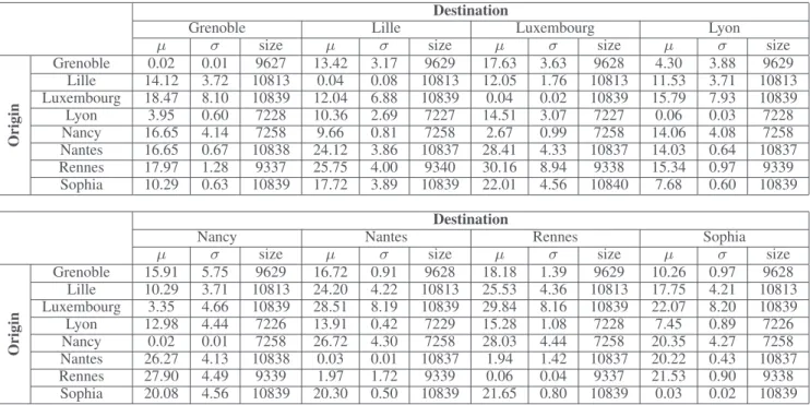
Statistics (mean, standard deviation, and dataset size) re-garding collected data are shown on Table I. Overall, collected data were quasi-symmetrical, i.e. measures from node A to

(5)

TABLE I: Statistics summary of raw RTTs collected in Grid’5000 Destination

Grenoble Lille Luxembourg Lyon µ σ size µ σ size µ σ size µ σ size

Origin Grenoble 0.02 0.01 9627 13.42 3.17 9629 17.63 3.63 9628 4.30 3.88 9629 Lille 14.12 3.72 10813 0.04 0.08 10813 12.05 1.76 10813 11.53 3.71 10813 Luxembourg 18.47 8.10 10839 12.04 6.88 10839 0.04 0.02 10839 15.79 7.93 10839 Lyon 3.95 0.60 7228 10.36 2.69 7227 14.51 3.07 7227 0.06 0.03 7228 Nancy 16.65 4.14 7258 9.66 0.81 7258 2.67 0.99 7258 14.06 4.08 7258 Nantes 16.65 0.67 10838 24.12 3.86 10837 28.41 4.33 10837 14.03 0.64 10837 Rennes 17.97 1.28 9337 25.75 4.00 9340 30.16 8.94 9338 15.34 0.97 9339 Sophia 10.29 0.63 10839 17.72 3.89 10839 22.01 4.56 10840 7.68 0.60 10839 Destination

Nancy Nantes Rennes Sophia

µ σ size µ σ size µ σ size µ σ size

Origin Grenoble 15.91 5.75 9629 16.72 0.91 9628 18.18 1.39 9629 10.26 0.97 9628 Lille 10.29 3.71 10813 24.20 4.22 10813 25.53 4.36 10813 17.75 4.21 10813 Luxembourg 3.35 4.66 10839 28.51 8.19 10839 29.84 8.16 10839 22.07 8.20 10839 Lyon 12.98 4.44 7226 13.91 0.42 7229 15.28 1.08 7228 7.45 0.89 7226 Nancy 0.02 0.01 7258 26.72 4.30 7258 28.03 4.44 7258 20.35 4.27 7258 Nantes 26.27 4.13 10838 0.03 0.01 10837 1.94 1.42 10837 20.22 0.43 10837 Rennes 27.90 4.49 9339 1.97 1.72 9339 0.06 0.04 9337 21.53 0.90 9338 Sophia 20.08 4.56 10839 20.30 0.50 10839 21.65 0.80 10839 0.03 0.02 10839

another node B are similar to those from node B to node A as it can be seen on Table I. Also, we did not consider collected hop counts in location verification, because their values are static due to dedicated connections established through Grid’5000 platform: hop count is either 1 when a front-end server interact with itself or 3 when it interacts with another node.

B. Dataset preprocessing

Being a free public research platform, some frontend nodes on which our scripts were running could be rebooted without any warning. Consequently, some measures were missing leading to different sizes in subsets associated with different couples of nodes as shown on Table I. To provide the same conditions for evaluated VDL approaches, we first discarded measures for some nodes (Lyon and Nancy nodes, because the ratio of missing measures is high; see Table I). Then, we discarded outliers, like those samples with hop count greater than 3 or RTT values higher than 100 ms, which result in abnormal routing in Grid’5000. Finally, we synchronized the remaining measures for each originating city. Synchronization is based on sample timestamps, with a certain error margin due to the scripts being distributed. Measures are kept when they are sampled in the same time interval for all the city nodes. After preprocessing, the dataset included 172,392 samples.

C. Learning algorithms comparison

Supervised machine learning is based on two steps: training to build a model and prediction to provide results to user. DLV approaches mainly differ in their learning process. The prediction is similar for approaches we considered, it consists in feeding data—i.e. collected RTTs without location, i.e.

without labels—to built model and let it return a result, i.e. a predicted location.

Training in bestline-based and linear regression-based ap-proaches consists in building the distance prediction functions using bestline and linear regression functions, respectively. One function is produced per node, using all requests issued by such a node to probe other nodes.

In the polynomial-based approach, a single prediction func-tion is needed; it is obtained by polynomial regression on the entire dataset, as done in [7].

In prediction step, distance estimate model is applied to new samples collected from known origins. Returned estimate distance is mapped to a circle for each node, which collected test data. Circle centers are location coordinates of nodes.

Then, approximation of circles as polygons of 10,000 points are derived and intersections of all polygons are calculated. The final result is a polygon representing a geographic zone in which the data are expected to be located. When multilat-eration result is perfect, all circles intersect at a single point, which is the location of CSP. However, due to fluctuations in collected RTTs, we address estimated distances as a maximum boundary, thus the intersection is a zone.

To use DLV methods, one has to specify the zone where data are accepted to be located, which is called accepted

zone. There are different ways to describe accepted zone including names (of cities, countries, states... ), geometric forms, geographic points... To apply multilateration in our context, we associate a circle to each node in Grid’5000 platform; circle centers are coordinates of buildings hosting Grid’5000 nodes in considered cities.

(6)

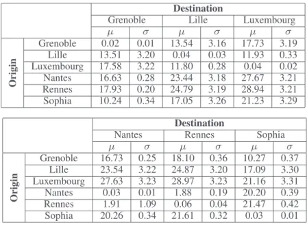
TABLE II: Statistics summary of preprocessed RTTs (Dataset with 172,392 samples) Destination

Grenoble Lille Luxembourg

µ σ µ σ µ σ Origin Grenoble 0.02 0.01 13.54 3.16 17.73 3.19 Lille 13.51 3.20 0.04 0.03 11.93 0.33 Luxembourg 17.58 3.22 11.80 0.28 0.04 0.02 Nantes 16.63 0.28 23.44 3.18 27.67 3.21 Rennes 17.93 0.20 24.79 3.19 28.94 3.21 Sophia 10.24 0.34 17.05 3.26 21.23 3.29 Destination

Nantes Rennes Sophia

µ σ µ σ µ σ Origin Grenoble 16.73 0.25 18.10 0.36 10.27 0.37 Lille 23.54 3.22 24.87 3.20 17.09 3.30 Luxembourg 27.63 3.23 28.97 3.23 21.16 3.31 Nantes 0.03 0.01 1.88 0.19 20.20 0.39 Rennes 1.91 1.09 0.06 0.04 21.47 0.42 Sophia 20.26 0.34 21.61 0.32 0.03 0.01

display multilateration result as shown on Figures 2, 3, and 4. In blue is estimate zone, in red is accepted zone, and in green is the intersection of both zones.

To assess estimate results, we use three scores:

• Verification consensus score, a verification consensus

score vcsi is associated with each prediction test i; it

equals the ratio of the maximum of number of intersect-ing estimated zones to the total number of landmarks participating in the verification. vcsi equals 0 means

that landmarks failed a have any consensus on common estimated zone. Then, an average success score, denoted VCS_{, is computed for all tests for each DLV approach;}

Ntis the number of tests:

vcs_i= Maximum number of intersecting estimated zones Number of landmarks participating in verification

V CS = 1 N t N t X i=1 vcs_i

• Inclusion ratio score, denoted IRS, is ratio of the

inter-section between predicted and accepted zones to accepted zone. IRS indicates the proportion of accepted zone covered by estimated zone.

I RS = Accepted zone∩ Estimated zone Accepted zone

• Estimate accuracy score, denoted EAS, is the ratio of

the intersection between predicted and accepted zones to predicted zone. EAS indicates the proportion of estimated zone covered by accepted zone.

EAS = Accepted zone∩ Estimated zone Estimated zone

VCS, IRS, and EAS together provide useful details to assess DLV algorithms. VCS alone reflects the percentage of land-marks, which agreed on a common zone. Unfortunately, they

may agree on a zone without intersection with the expected zone. IRS alone is not enough. Let us take an example. Imagine that accepted zone is a 1km-radium-circle entirely included in an estimated zone covered by a 10km-radium-circle. In this case, IRS equals 1.00. However, as the size of estimated zone is 100 times the one of accepted zone, the data could be located out of the accepted zone. EAS is 1%, which means that the location verification accuracy is very low. EAS alone also is not enough. Let us take the following scenarios: i) estimated and accepted zones are 100 km2 _{and intersect at}

50%, resulting in a zone of 50 km2_{of unauthorized zone where}

the data may be located, ii) if both zone sizes are heightened with a factor F, EAS remains 50%, but the unauthorized zone is heightened with the same factor. Consequently, in addition to scores, the size of estimated zone is useful to user to assess the verification result. User derives the estimated zone from IRS, EAS, and accepted zone.

D. Experimentation scenarios

To provide significant results to assess DLV approaches, we carried out multiple scenarios designed as follows:

• Varying ratio between training and test sets: three

alter-natives for splitting the dataset into training and test sets are considered: 0.8/0.2, 0.5/0.5, and 0.2/0.8.

• Varying accepted zone scale: four alternatives of

ac-cepted zone size are considered: 10 km (city scale), 50 km (metropolis-and-surroundings scale), 200 km (region scale), and 500 km (country scale).

• Varying the degree in polynomial regression until no

result improvement is observed.

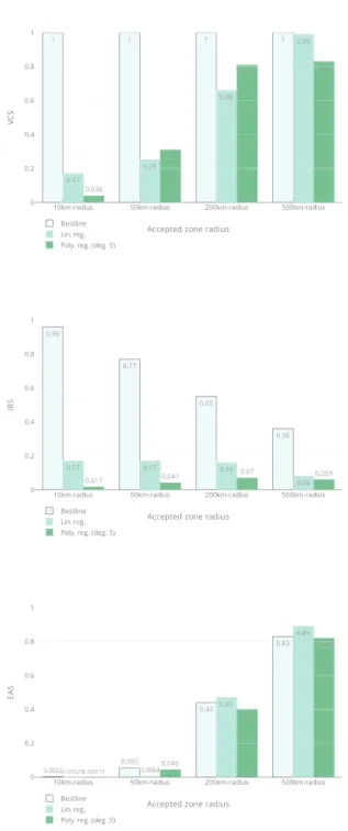
Experimentation results for 0.5/0.5 train/test ratio are sum-marized in Figure 5. Notice that histograms are associated with VCS with unanimity (i.e. all estimated zones intersect in a common non-empty zone).

(7)

Fig. 2: Example of output for bestline-based DLV. The green polygon is the intersection between the predicted zone us in blue, and the accepted zone around Lille in red.

Fig. 3: Example of output for linear regression based DLV. The blue zone is the predicted one. In this case it did not succeed in predicting location (Lille)

IV. CONCLUSION

In this paper, we report on an experimentation of data loca-tion verificaloca-tion approaches based on regression and bestline. Experimentation is based on Grid5000, which is a national communication infrastructure connecting the main cities in France. During a month, measurements of RTTs have been collected by landmarks located at different cities. Then, three verification approaches (bestline, linear regression, and

poly-Fig. 4: Example of output for polynomial regression based DLV. There is no resulting zone because circles do not intersect. Circles are denoted in grey with a location marker at their centers, there is one in Sophia (the big one) and one in Rennes. As there is no resulting zone, it fails to prediction location (Nantes)

nomial regression) have been assessed. Hopeful results have been observed, meaning that landmark-based verification ap-proaches are credible solutions to locate data at country-scale. Bestline-based approach has a high Verification consensus score (because it overestimates distance) but a low accuracy, because of the size of estimated zone. Linear regression-based approach outperforms polynomial regression-based approach when all landmarks use the same polynomial. Whenever each landmark uses its own polynomial the reverse performance is observed. Regression-based approaches tend to optimize the distance estimate model, which, unfortunately, results in smaller estimated zones, which are unlikely to intersect in a common zone. Even when the expected zone is large, the localization success may be low.

In our current work, we are analyzing the compromise between accuracy of distance model of individual landmarks and the size of expected zone for which the localization success would be high. For future work, we are extending our analysis by collecting and experimenting a worldwide dataset. We would also like to include classification-based approaches in our performance analysis.

REFERENCES

[1] A. Albeshri, C. Boyd, and J. G. Nieto. Geoproof: Proofs of geographic location for cloud computing environment. In Distributed Computing

Systems Workshops (ICDCSW), 2012 32nd International Conference on, pages 506–514, June 2012.

[2] Daniel Balouek, Alexandra Carpen Amarie, Ghislain Charrier, Frédéric Desprez, Emmanuel Jeannot, Emmanuel Jeanvoine, Adrien Lèbre, David Margery, Nicolas Niclausse, Lucas Nussbaum, Olivier Richard, Christian Pérez, Flavien Quesnel, Cyril Rohr, and Luc Sarzyniec. Adding

(8)

1 1 1 1 0.17 0.25 0.25 0.66 0.99 0.038 0.31 0.81 0.830.83

10km-radius 50km-radius 200km-radius 500km-radius

0 0.2 0.4 0.6 0.8 1 Bestline Bestline Lin. reg. Lin. reg. Poly. reg. (deg. 5) Poly. reg. (deg. 5)

Accepted zone radius

V C S 0.96 0.77 0.55 0.36 0.17 0.17 0.16 0.08 0.017 0.041 0.07 0.059

IR S 0.0032 0.055 0.44 0.44 0.83 0.83 0.00025 0.0064 0.47 0.89 0.00072 0.00025 0.00025 0.045 0.4 0.82

E

A

S

Fig. 5: Scores for a 0.5/0.5 train/test ratio with 10km, 50km, 200km and 500km-radii accepted zone scales. (VCS is in-creased only when all estimated zones intersect

virtualization capabilities to the Grid’5000 testbed. In Ivan I. Ivanov, Marten van Sinderen, Frank Leymann, and Tony Shan, editors, Cloud

Computing and Services Science, volume 367 of Communications in

Computer and Information Science, pages 3–20. Springer International Publishing, 2013.

[3] Michael Bartock, Murugiah Souppaya, Raghuram Yeluri, Uttam Shetty, James Greene, Steve Orrin, Hemma Prafullchandra, John McLeese, Jason Mills, Daniel Carayiannis, et al. Trusted geolocation in the cloud: Proof of concept implementation. Nat. Instit. Stand. Technol. Internal

Report 7904, 2015.

[4] Karyn Benson, Rafael Dowsley, and Hovav Shacham. Do you know where your cloud files are? In Proceedings of the 3rd ACM Workshop

on Cloud Computing Security Workshop, CCSW ’11, pages 73–82, New York, NY, USA, 2011. ACM.

[5] S. Betg´e-Brezetz, G. B. Kamga, M. P. Dupont, and A. Guesmi. Privacy control in cloud vm file systems. In Cloud Computing Technology

and Science (CloudCom), 2013 IEEE 5th International Conference on, volume 2, pages 276–280, Dec 2013.

[6] B. Biswal, S. Shetty, and T. Rogers. Enhanced learning classifier to locate data in cloud datacenters. In Cloud Networking (CloudNet), 2014

IEEE 3rd International Conference on, pages 375–380, Oct 2014. [7] M. Eskandari, A. S. D. Oliveira, and B. Crispo. Vloc: An approach

to verify the physical location of a virtual machine in cloud. In

Cloud Computing Technology and Science (CloudCom), 2014 IEEE 6th International Conference on, pages 86–94, Dec 2014.

[8] M. Fotouhi, A. Anand, and R. Hasan. Plag: Practical landmark allocation for cloud geolocation. In Cloud Computing (CLOUD), 2015 IEEE 8th

International Conference on, pages 1103–1106, June 2015.

[9] Mark Gondree and Zachary N.J. Peterson. Geolocation of data in the cloud. In Proceedings of the Third ACM Conference on Data and

Application Security and Privacy, CODASPY ’13, pages 25–36, New York, NY, USA, 2013. ACM.

[10] Regulation (eu) 2016/679 of the european parliament and of the council of 27 april 2016 on the protection of natural persons with regard to the processing of personal data and on the free movement of such data, and repealing directive 95/46/ec (general data protection regu-lation). http://eur-lex.europa.eu/legal-content/EN/TXT/?uri=CELEX% 3A32016R0679. Accessed: 13 September 2018.

[11] Usa: Health insurance portability and accountability act. https://www. gpo.gov/fdsys/pkg/PLAW-104publ191/html/PLAW-104publ191.htm. Accessed: 13 September 2018.

[12] Malik Irain, Jacques Jorda, and Zoubir Mammeri. Landmark-based data location verification in the cloud: review of approaches and challenges.

Journal of Cloud Computing, 6(1):31, Dec 2017.

[13] C. Jaiswal and V. Kumar. Igod: Identification of geolocation of cloud datacenters. In 2015 IEEE 40th Local Computer Networks Conference

Workshops (LCN Workshops), pages 665–672, Oct 2015.

[14] Christoph Krauß and Volker Fusenig. Network and System Security: 7th

International Conference, NSS 2013, Madrid, Spain, June 3-4, 2013. Proceedings, chapter Using Trusted Platform Modules for Location Assurance in Cloud Networking, pages 109–121. Springer Berlin Heidelberg, Berlin, Heidelberg, 2013.

[15] P. Massonet, S. Naqvi, C. Ponsard, J. Latanicki, B. Rochwerger, and M. Villari. A monitoring and audit logging architecture for data location compliance in federated cloud infrastructures. In Parallel and

Distributed Processing Workshops and Phd Forum (IPDPSW), 2011 IEEE International Symposium on, pages 1510–1517, May 2011. [16] Canada: Personal information protection and electronic documents act.

http://laws-lois.justice.gc.ca/eng/acts/P-8.6/. Accessed: 13 September 2018.

[17] T. Ries, V. Fusenig, C. Vilbois, and T. Engel. Verification of data location in cloud networking. In 2011 Fourth IEEE International Conference on

Utility and Cloud Computing, pages 439–444, Dec 2011.

[18] Gaven J. Watson, Reihaneh Safavi-Naini, Mohsen Alimomeni, Michael E. Locasto, and Shivaramakrishnan Narayan. Lost: Location based storage. In Proceedings of the 2012 ACM Workshop on Cloud

Computing Security Workshop, CCSW ’12, pages 59–70, New York, NY, USA, 2012. ACM.

[19] T. W¨uchner, S. M¨uller, and R. Fischer. Compliance-preserving cloud storage federation based on data-driven usage control. In Cloud

Comput-ing Technology and Science (CloudCom), 2013 IEEE 5th International Conference on, volume 2, pages 285–288, Dec 2013.