HAL Id: hal-01940174
https://hal.archives-ouvertes.fr/hal-01940174
Submitted on 30 Nov 2018
HAL is a multi-disciplinary open access
archive for the deposit and dissemination of
sci-entific research documents, whether they are
pub-lished or not. The documents may come from
teaching and research institutions in France or
abroad, or from public or private research centers.
L’archive ouverte pluridisciplinaire HAL, est
destinée au dépôt et à la diffusion de documents
scientifiques de niveau recherche, publiés ou non,
émanant des établissements d’enseignement et de
recherche français ou étrangers, des laboratoires
publics ou privés.
Combining Refinement of Parametric Models with
Goal-Oriented Reduction of Dynamics
Stefan Haar, Juraj Kolčák, Loïc Paulevé
To cite this version:
Stefan Haar, Juraj Kolčák, Loïc Paulevé. Combining Refinement of Parametric Models with
Goal-Oriented Reduction of Dynamics. VMCAI 2019 - 20th International Conference on Verification, Model
Checking, and Abstract Interpretation, Jan 2019, Lisbon, Portugal. pp.555-576,
�10.1007/978-3-030-11245-5_26�. �hal-01940174�
Combining Refinement of Parametric Models
with Goal-Oriented Reduction of Dynamics
?Stefan Haar1, Juraj Kolčák1,2, Loïc Paulevé3,4
1
LSV, CNRS & ENS Paris-Saclay, Université Paris-Saclay, France
2
National Institute of Informatics, Tokyo, Japan
3
LRI UMR 8623, Univ. Paris-Sud – CNRS, Université Paris-Saclay, Orsay, France
4 Univ. Bordeaux, Bordeaux INP, CNRS, LaBRI, UMR5800, F-33400 Talence, France
Abstract Parametric models abstract part of the specification of dy-namical models by integral parameters. They are for example used in computational systems biology, notably with parametric regulatory works, which specify the global architecture (interactions) of the net-works, while parameterising the precise rules for drawing the possible temporal evolutions of the states of the components. A key challenge is then to identify the discrete parameters corresponding to concrete models with desired dynamical properties. This paper addresses the restriction of the abstract execution of parametric regulatory (discrete) networks by the means of static analysis of reachability properties (goal states). Initially defined at the level of concrete parameterised models, the goal-oriented reduction of dynamics is lifted to parametric networks, and is proven to preserve all the minimal traces to the specified goal states. It results that one can jointly perform the refinement of parametric net-works (restriction of domain of parameters) while reducing the necessary transitions to explore and preserving reachability properties of interest.
1
Introduction
Various cyber and physical systems are studied by the means of discrete dynam-ical models which describe the possible temporal evolution of the state of the components of the system. Defining such models requires extensive knowledge on the underlying system for specifying the rules which generate the admiss-ible state transitions over time. Usually, and especially for physical systems, such as biological networks for which discrete models are extensively employed [24,12,8,1,9,18], it is common to lack such precise knowledge, making an accurate specification of discrete models challenging.
With parametric models, part of the specification of the rules for generating the discrete transitions is encoded as (integral) parameters. Thus, a parametric
?
This work has been partly funded by ANR-FNR project “AlgoReCell” ANR-16-CE12-0034, by Labex DigiCosme (project ANR-11-LABEX-0045-DIGICOSME) op-erated by ANR as part of the program “Investissement d’Avenir” Idex Paris-Saclay (ANR-11-IDEX-0003-02), and by ERATO HASUO Metamathematics for Systems Design Project (No. JPMJER 1603), JST.
model abstracts a set of concrete parameterised models, this set being charac-terised by the domain of parameter values.
In this paper, we focus on Parametric Regulatory Networks (PRNs), also known as Thomas Networks [23,4,2,15], which are commonly employed for mod-elling qualitative dynamics of biological systems. PRNs allow separating biolo-gical knowledge on the pairwise interactions (the architecture of the network) from the rules of interplay between the interactions, usually less known.
In the literature, PRNs are mainly used as a basic framework for identifying fully parameterised models (i.e., Boolean and multilevel networks) which satisfy dynamical properties typically generated from experimental data. This identific-ation task, related to so-called model inference and process mining [5,17,16,21], consists in transforming an abstract parametric model into a set of concrete para-meterised models verifying desired dynamical properties. For PRNs, state-of-the-art methods rely on parameter enumeration [13], coloured model-checking [14], logic programming and Boolean satisfiability [10,19], and Hoare logic [3].
However, the exhaustive identification of parameters is often limited to small models, as the set of parameterised models can turn out to be too large to be exhaustively enumerated and further analysed.
In [15], we introduced a semantics of PRNs enabling the refinement of a PRN by restricting the domain of its parameters without having to enumerate concrete models, keeping them in a compact abstract representation instead. The refinement is performed according to concrete discrete state transitions: the domain of parameters is restricted so that it abstracts all the concrete models in which the state transition is admissible. Essentially, such semantics of PRNs enable efficient exploration of dynamics of a set of parameterised models.
This exploration suffers from the same bottleneck as individual parameterised models: the number of reachable states grows exponentially with the number of components and thus, becomes intractable for large networks. The exploration of the reachable state space is usually performed to verify dynamical properties. Consequently, various model reduction methods have been designed on concrete parameterised models to enhance the tractability of their verification [11,22,20,6]: by reducing the transitions to consider, these methods limit the reachable state space to explore while guaranteeing the correctness of the verification.
In this paper, we address the combination of refinement operations on para-metric models with model reductions initially defined at the level of concrete individual models. Essentially, the challenge consists in lifting up such model reductions so they can be performed at the abstract level of parametric models, while ensuring the correctness of their refinement.
We focus on reachability properties, i.e., starting in an initial configuration, the ability to eventually reach a given (partial) configuration. On the one hand, we are interested in refining PRNs to accurately identify concrete parameterised discrete network models that verify the reachability property; on the other hand, we want to take advantage of goal-driven exploration of dynamics of paramet-erised models to ignore transitions which do not influence the reachability of the goal, enhancing the tractability of the analysis.
The refinement of PRNs we consider for reachability properties has been introduced in [15]. It consists in dynamically drawing transitions allowed by at least one concrete model, and subsequently restricts the domain of parameters to exclude models which do not allow the drawn transition. The generation of transitions is done directly from the abstract representation of the set of concrete models, and therefore involves no enumeration of parameterised models.
The goal-oriented model reduction we consider has been introduced in [20] at the level of parameterised network models. Given a reachability property (goal), the method relies on static analysis by abstract interpretation to identify trans-itions which are not involved in any minimal trace leading to the goal. Here the minimality refers to the absence of a sub-trace. Whereas deciding reachability properties in parametrised models (namely automata networks) is a PSPACE-complete problem [7], the goal-oriented model reduction has a complexity poly-nomial in the number of components and exponential in the in-degree of com-ponents in the networks (comcom-ponents having a direct influence on a single one). In this article we present a lifting of the goal-oriented reduction from metrised models to sets of models with shared architecture, represented by para-metric models. To this end, we introduce a directed version of PRNs which allow us to efficiently capture model reduction without the need to explicitly enumer-ate all possible transitions. We conduct the reduction itself on abstract dynamics of PRNs where instead of enumerating all enabled transitions, we only consider the minimal necessary condition for each component to change value.
The introduced reduction method can be applied on-the-fly to speed up reach-ability checking in parametric models. Thanks to the preservation of all minimal traces, it is guaranteed to capture all parametrised models capable of reprodu-cing the coveted behaviour.
Outline Section 2 recalls the definition of parametric regulatory networks, their dynamics, constraints on influences and finally presents a generalised paramet-risation set semantics. In Section 3, the goal-oriented model reduction procedure is extended from parametrised models to parametric models. Directed version of PRNs is introduced for this purpose alongside an abstraction of dynamics de-signed to alleviate the reduction complexity. Section 4 supplies an algorithm for computing a suitable abstraction of PRN dynamics used in the reduction pro-cedure. Finally, Section 5 summarises the results and offers a brief introduction to possible extensions and applications as well as future directions.
Notations We useQ to build Cartesian products between sets. As the ordering of components matters, Q is not commutative. Therefore, we write Q≤x∈X for the product over elements in X according to a total order ≤. To ease notations, when the order is clear from the context, or when either X is a set of integers, or a set of integer vectors, on which we use the lexicographic ordering, we simply write Q
x∈X. Given a sequence of n elements π = (πi)1≤i≤n, we write πe
∆
= {πi| 1 ≤ i ≤ n} for the set of its elements. Given a vector v = hv1, . . . , vni, we
write v[i7→y] for the vector equal to v except on the component i, which is equal
2
Parametric Regulatory Networks
Regulatory networks are finite discrete dynamical systems where the components evolve individually with respect to the value of (a few) other components, their regulators. The value of components in regulatory networks ranges in a finite discrete domain, usually represented as {0, ..., m} for some m ∈ N, thus extending Boolean networks [24]. The evolution of components is then defined by discrete functions which associate to the global states of the network the value towards which each component tends.
Thus, defining regulatory networks requires knowledge on which components influence each others, and how the value of each component is computed from the value of its regulators. Parametric Regulatory Networks (PRNs) allow to decouple this specification by having on the one hand a fixed architecture of the network, so-called influence graph, and on the other hand discrete parameters, which when instantiated specify the functions of the regulatory network. 2.1 Influence graph and constraints
The influence graph encodes the directed interactions between the components of the regulatory networks: a component u having a direct influence on component v means that in some states of the regulatory network, the computation of the value of node v may depend on the value of u. Importantly, if the component w has no direct influence of v, then the computation of the value on v never depends on the value of w.
Definition 1 (Influence Graph). An influence graph G is a tuple (V, I) where V is a finite set of n nodes (components) and I ⊆ V × V is a set of directed edges (influences).
For each v ∈ V we denote the set of its regulators by n−(v)= {u ∈ V | (u, v) ∈ I}.∆ Besides the existence/absence of direct influences between components, it is usual to have some knowledge about the nature of the influences. Two kinds of constraints are generally considered: signs and observability.
Influence signs are captured by monotonicity constraints. An influence (u, v) ∈ I is positive-monotonic, denoted +, if the sole increase of the value of the reg-ulator u cannot cause a decrease of the computed value of the target v. Sym-metrically, an influence (u, v) ∈ I is negative-monotonic, denoted −, if the sole increase in the value of u cannot cause an increase in the computed value of v. An influence (u, v) ∈ I is observable, denoted o, if there exists a state in which the sole change of the value of u induces a change of the computed value of v. Thus observability enforces that u does have an influence on the value of v, in some states of the regulatory network. Remark that observability does not imply positive/negative monotonicity – e.g., when the value of v is computed as the exclusive disjunction XOR between its own value and the value of u.
Let us denote a set of influence constraints for an influence graph (V, I) as R ⊆ I × {+, −, o}. An example of influence constraint set is given in Figure 1 (a) as labels on edges of the influence graph.
2.2 Parametrisation
Let us consider an influence graph G = (V, I) among n components and a set of influences constraints R. Let us denote by m ∈ Nn the vector specifying the maximum discrete value of each component: the states of the regulator networks span Q
v∈V{0, . . . , mv}. The computation of the value of each component of a
regulatory network is constrained by G, R and m. In particular, G imposes that the value of a component depends only on its regulators.
A regulator state ω of a component v ∈ V is a vector specifying the value of each regulator of v. We denote the set of all regulator states of a component as Ωv
∆
=Q
u∈n−(v){0, . . . , mu}. Intuitively, a regulator state of a component v is a
projection of a global state of the network (states of all components) to just the regulators of v, that fully determine its evolution.
A parameter hv, ωi then represents a target value towards which component v ∈ V evolves in regulator state ω ∈ Ωv. We denote the set of all parameters as
Ω∆=S
v∈V{v} × Ωv
A parametrisation P is a vector assigning a value to each parameter. The set of all parametrisations associated to an influence graph G and a maximum value vector m is therefore given by P(Gm) =QEhv,ωi∈Ω{0, . . . , mv} where E is
an arbitrary, but fixed total order on parameters. The set of all parametrisations satisfying both the influence graph G = (V, I) and influence constraints R with maximum value vector m is then defined as:
P(GRm) ∆
= {P ∈QE
hv,ωi∈Ω{0, . . . , mv} | ∀u, v ∈ V,
(u, v, +) ∈ R ⇒ ∀ω ∈ Ωv, ∀k ∈ {1, . . . , mu} : Pv,ω[u7→k] ≥ Pv,ω[u7→k−1]
(u, v, −) ∈ R ⇒ ∀ω ∈ Ωv, ∀k ∈ {1, . . . , mu} : Pv,ω
[u7→k] ≤ Pv,ω[u7→k−1]
(u, v, o) ∈ R ⇒ ∃ω ∈ Ωv, ∃k ∈ {1, . . . , mu} : Pv,ω[u7→k] 6= Pv,ω[u7→k−1]}
2.3 Parametric Regulatory Networks
A Parametric Regulatory Network (PRN) gathers an influence graph G, influence constraints R, and maximum value vector m, to which can then be associated a subset of parametrisations P(GR
m). A (parametrised ) regulatory network can
then be defined by a couple (GR
m, P ) where P ∈ P(GRm).
Definition 2. A parametric regulatory network (PRN) is a tuple (G, m, R), written GRm, where G is an influence graph between n components, R is a set of
influence constraints, and m ∈ Nn is a vector of the maximum values of each component.
The set of states of GR
m is denoted by S(GRm) ∆
=Q
v∈V{0, . . . , mv}.
The set of (local) transitions of GRm is denoted by: ∆(GRm) = {(v∆ i→ vj, ω) |
v ∈ V ∧ ω ∈ Ωv∧ i, j ∈ {0, . . . , mv} ∧ |i − j| = 1}. We use V ((vi→ vj, ω)) = v
to denote the component whose value is changed by transition (vi→ vj, ω) ∈
∆(GRm). Furthermore, s((vi→ vj, ω)) = s(vi→ vj) = j − i denotes the sign of
A transition (vi→ vj, ω) ∈ ∆(GRm) is enabled in state x ∈ S(GRm) if xv = i
and ωv(x) = ω, where ωv(x) is the projection of state x to the regulators of v.
Given a state x and a transition t enabled in x, x · t denotes the state x[v7→j]∈
S(GRm) obtained by firing transition t in x.
Finally, a transition (vi → vj, ω) ∈ ∆(GRm) is enabled by a parametrisation
set P ⊆ P(GRm) if there exists a parametrisation P ∈ P such that the parameter
value Pv,ω = j + a · s(vi→ vj) for some a ∈ N0.
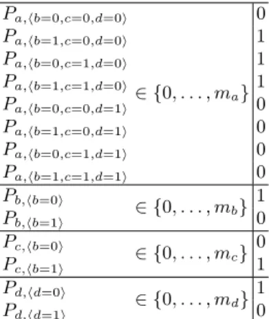
Example 1. An example of a PRN GR
mcomposed of an influence graph G = (V, I)
and vector m = {1}|V |is depicted in Figure 1. Based on the influences in G and maximum values in m, all regulator states of each component, which correspond to parameters of GR
m, are determined. The table in Figure 1 (b) lists all the
para-meters alongside an example parametrisation P ∈ P(GRm). G R
m combined with
P identifies a unique parametrised network (GRm, P ). The dynamics of (GRm, P )
are given in Figure 1 (c).
We capture the basic semantics of a PRN by traces, which correspond to different possible behaviours of the network.
Definition 3 (Trace). Given a PRN GR
m and set of parametrisations P ⊆
P(GRm), a finite sequence π = (π1, . . . , π|π|) of transitions in ∆(GRm) is a trace
of GR
m starting in state x ∈ S(GRm) iff ∀i ∈ {1, . . . , |π|} : πi is enabled in state
x · π1· . . . · πi−1 and by parametrisation set P.
To simplify notation, we use•π = x and π•= x · π1· . . . · π|π|. Moreover, let
π:i = (π
1, . . . , πi), πi:= (πi, . . . , π|π|) and πi:j = (πi, . . . , πj) denote the prefix,
suffix and infix sub-traces of π respectively. With P ∈ P(GR
m) and P = {P }, the above definition gives the traces of the
parametrised regulatory network (GR
m, P ). In the general case, each transition is
independently enabled with respect to any parametrisation in P. 2.4 Parametrisation Set Semantics
With the basic PRN semantics (Definition 3), two transitions are allowed to fire consequently in a single trace despite no single parametrisation enabling both of them. To forbid such behaviours, semantics have been introduced for PRNs that associate each trace (set of transitions) with a set of parametrisations [15]. Said trace can then be extended only by transitions enabled under some para-metrisation from the associated set.
The purpose of parametrisation set semantics is to discriminate transitions based on their causal history. This is done by progressive restriction of the set of parametrisations to admissible parametrisations. Following [15], we consider a parametrisation P to be admissible if all transitions in the set (causal history) are enabled under P . However, we allow for a more lenient definition to make room for over-approximation.
Definition 4 (Parametrisation Set Semantics). Given a PRN GR
m, a
func-tion Ψ : 2∆(GRm)→ 2P(GRm) is a parametrisation set semantics of GR
a b c d −o −o +o + −o +o
(a) The influence graph G.
Pa,hb=0,c=0,d=0i ∈ {0, . . . , ma} 0 Pa,hb=1,c=0,d=0i 1 Pa,hb=0,c=1,d=0i 1 Pa,hb=1,c=1,d=0i 1 Pa,hb=0,c=0,d=1i 0 Pa,hb=1,c=0,d=1i 0 Pa,hb=0,c=1,d=1i 0 Pa,hb=1,c=1,d=1i 0 Pb,hb=0i ∈ {0, . . . , m b} 1 Pb,hb=1i 0 Pc,hb=0i ∈ {0, . . . , mc} 0 Pc,hb=1i 1 Pd,hd=0i ∈ {0, . . . , m d} 1 Pd,hd=1i 0
(b) All the parameters of PRN GRm
with an example parametrisation P .
0000 1000 0001 1001 0010 1010 0011 1011 0100 1100 0101 1101 0110 1110 0111 1111 b+ b− b+ b− d+ d− d+ d− c+ c+ c+ c+ c− c− c− c− a+ a+ a+ a− a− a− a− a−
(c) States and transitions of (GR
m, P ) depicted as nodes and edges of a
state space graph respectively. Since components b and d may update values independently of other components (i.e. in any state), their value changes are only displayed schematically to improve readability.
Figure 1: Influence graph with influence constraints as labels, parameters and dynamics of a possible parametrisation of PRN GR
m.
1. ∀T ⊆ ∆(GR
m) : {P ∈ P(GRm) | ∀t ∈ T : P enables t} ⊆ Ψ (T ),
2. ∀T, T0 ⊆ ∆(GR
m) : T ⊆ T0⇒ Ψ (T0) ⊆ Ψ (T ).
A trace π of the PRN GRm is realisable according to the parametrisation set
semantics if and only if Ψ (π) 6= ∅.e
A best abstraction ΨCproducing parametrisation sets of exactly all the
para-metrisations that allow each transition in the input set has been defined in [15]. To facilitate practical application, as the number of parametrisations may be in the worst case double exponential in the number of components, [15] has
tackled the semantics ΨA over-approximating parametrisation sets by convex
covers, keeping track of only a maximal and minimal element and thus avoiding the need to enumerate parametrisations explicitly. More formally, let us first reintroduce the parametrisation order.
Definition 5. The parametrisation order on vectors of length k is the partial order ≤ defined as follows:
a ≤ b⇔ ∀i ∈ {0, . . . , k − 1} : a∆ i≤ bi
The parametrisation set given by ΨA is a couple of parametrisations (L, U )
representing the lower and upper bound. Formally, (L, U ) = {P ∈ P(GR m) |
L ≤ P ∧ U ≥ P } is a bounded convex sublattice of all vectors of length |Ω| with the parametrisation order. In [15], a method has been provided to compute the tightest lower and upper bounds for a given set of transitions and influence constraints without the need to explicitly enumerate the parametrisations.
Naturally, checking whether a particular parametrisation belongs to the ab-stracted set can be done simply by comparing it with the bounds. Similarly, determining whether a transition is enabled (by any parametrisation) can be done without explicit enumeration of the parametrisations. In fact, it is enough to compare against the corresponding parameter value of the relevant bound, e.g. Uv,ω ≥ k + 1 is the sufficient and necessary condition for the transition
(vk → vk+1, ω) to be enabled.
In this article, we consider any parametrisation set semantics compatible with Definition 4, however, special attention is given to ΨA as it can be used
with the restriction method without the need to enumerate the parametrisations explicitly.
3
Goal-Oriented Reduction
In this section, we extend the goal-oriented model reduction procedure from parametrised models (in particular, automata networks) [20] to the parametric models.
3.1 Minimal Traces
Given a PRN GRmand a state x ∈ S(GRm), we say a value > ∈ {0, . . . , mg} of a
component g ∈ V is reachable from x iff either xg= > or there exists a realisable
trace π with •π = x and π•g= >.
We are interested in reachability by minimal traces. Adapted from [20], a realisable trace is minimal for g> reachability if there exists no other realisable
trace reaching g> with a subsequence of transitions.
Definition 6 (Minimal Trace). Given a parametrised PRN (GRm, P ), a trace
there exists no other trace ρ satisfying x =•ρ, ρ•g= >, |ρ| < |π| and existence of an injection φ : {1, . . . , |ρ|} → {1, . . . , |π|} such that ∀i, j ∈ {1, . . . , |ρ|} : i ≤ j ⇒ φ(i) ≤ φ(j) and ρi= πφ(i).
An important property of minimal traces is their independence on the exact parametrisation. More precisely, using parametrisation set semantics, if a trace is minimal for at least one parametrisation, then it is minimal for any other parametrisation under which it is enabled.
Property 1 (Parametrisation Independence of Minimal Traces). Let GRm be a PRN and π a realisable trace minimal in (GRm, P ) for some P ∈ Ψ (eπ). Then, π is minimal in any (GRm, P0) where P0∈ Ψ (eπ)
Proof. P0 ∈ Ψ (eπ) guarantees π is a proper trace of (GR
m, P0). We conduct the
rest of the proof by contradiction. Let thus ρ be a trace in (GR
m, P0) satisfying
the conditions in Definition 6. From the existence of the injection φ we get e
ρ ⊆eπ and from the definition of parametrisation set semantics Ψ (eπ) ⊆ Ψ (ρ). ρ ise therefore realisable in (GR
m, P ) meaning that π is not minimal in (GRm, P ) which
is a contradiction.
Property 1 allows us to speak of a realisable trace of a PRN as minimal without the need to explicitly state the parametrisation which is witness to the minimality.
3.2 Directed Parametric Regulatory Networks
The goal-oriented reduction for parametrised models is facilitated by pruning transitions which are guaranteed to not be used by any minimal trace reaching the goal [20]. The PRN definition could be extended to allow for pruning the transition set to subsets T ⊆ ∆(GRm). Unlike the case of general parametrised
models, however, the transitions of a PRN only allow to change the value of a component by steps of size 1. As such, if a transition increasing the value of a component v ∈ V to k ∈ {0, . . . , mv} is to be pruned, all transitions
increas-ing the value of v beyond k can surely be pruned as well, and symmetrically for decreasing transitions. Thus, instead of removing individual transitions of PRNs, we disable increasing, respectively decreasing, value of a component in a given regulator state beyond a certain value (or entirely). This is facilitated by keeping record of the activation (increase) and inhibition (decrease) limits for each component in vectors lA and lI respectively.
Definition 7 (Directed Parametric Regulatory Network). A directed parametric regulatory network (DPRN) is a tuple G = (GRm, lA, lI), where GRm
is a parametric regulatory network, lA ∈ (N ∪ {−∞})|Ω| is a vector of
activa-tion limits for each regulator state ω ∈ Ω and lI ∈ (N0∪ {∞})|Ω| is a vector of
inhibition limits for each regulator state ω ∈ Ω.
The set of states of G is equal to the set of states of the underlying PRN: S(G) = S(GRm).
The set of transitions of G is a subset of the PRN transitions satisfying the activation and inhibition limits lAand lI respectively. Formally, ∆(G) ⊆ ∆(GRm) such that: ∀t = (vi→ vj, ω) ∈ ∆(GRm) : t ∈ ∆(G) ∆ ⇔ ( i < lAω if s(t) = +1 i > lI ω if s(t) = −1
One may remark that by using parametrisation set semantics, it is already possible to restrict the activation or inhibition of components in individual reg-ulator states while just using PRNs. While it is true that an equivalent set of enabled transitions can be achieved both by restricting the parametrisation set and by DPRN, the semantics of the two restrictions are different.
The parametrisation set semantics serves primarily to keep track of para-metrisations capable of reproducing certain behaviour(s), and thus restrict the set of enabled transitions based on their causal history. On the other hand, the lA and lI of DPRN mark components whose activation or inhibition (beyond a
certain value) is not necessary to reach a given goal (via a minimal trace). A parametrisation that allows changing a component value beyond the limit, thus allowing behaviour which does not lead to the established goal may still allow a different sequence of transitions leading to the goal. We want to retain such parametrisations, thus the "useless" behaviour which does not lead to the goal cannot be restricted in the parametrisation set semantics. Therefore, keeping the information about parametrisations and about the activation and inhibition limits independently is key.
The complete independence of parametrisation set semantics and the limit vectors lA and lI allows us to employ both in parallel. The extension of both traces (Definition 3) and parametrisation set semantics (Definition 4) from PRNs to DPRNs is thus natural.
3.3 Objectives
The reduction for parametrised models relies on identifying sub-goals, or object-ives, local in terms of individual components. We reintroduce the concept of a (local) objective for the parametric model.
Definition 8 (Objective). Given an DPRN G, an objective vi vj is a pair
of values i, j ∈ {0, . . . , mv} of a component v ∈ V .
An objective vi vj is valid in a starting state x ∈ S(G) iff i = j or a
realisable trace π of the parametrised DPRN exists, such that •π = x, π•v = j
and ∃k ∈ {0, . . . , |π| − 1} :•πk v= i.
i j is used to denote vi vj if the component v ∈ V is obvious from the
context.
Each objective vi vj captures either increase or decrease of the value of
the component. Formally, the sign of an objective s(vi vj) ∆
By requiring the witness of objective validity to be a realisable trace instead of just a trace of enabled transitions, we retain only behaviours which are present in at least one parametrised model.
The objective represents a change of value of only one component v ∈ V . A realisable trace reproducing such a change may, however, require to also change value of other components, namely the regulators of v. Each objective is thus associated to a set of transitions which may be used to complete it, and from which the required regulator values can be obtained.
3.4 Regulation Cover Sets
Depending on the parametrisation set semantics, it may be a common occur-rence for a particular value change to be enabled by numerous regulator states (recall that enabling is existential w.r.t. parametrisations). Such cases lead to a substantial redundancy in individual transition enumeration as the value of only a subset of regulators may be enough to determine whether a value change is enabled or not. To this end we introduce a definition of a partial regulator state, which is used to represent a (minimal) condition for a value change to be enabled.
Definition 9 (Partial Regulator State). A partial regulator state ℵ of com-ponent v ∈ V is a vector ℵ ∈Q
u∈n−(v){0, . . . , mu} ∪ {∗} assigning a value or a
wildcard character ∗ to each regulator u of v. By abuse of notation, ℵ is also a set of regulator states, more precisely ℵ ⊆ Ωv such that for all ω ∈ Ωv:
ω ∈ ℵ⇔ ∀u ∈ n∆ −(v) : ωu= ℵu∨ ℵu= ∗
The set of all partial regulator states of v ∈ V is denoted as Av.
Partial regulator states can be utilised to abstract the DPRN dynamics while minimising the number of repetitions of each value of each regulator. We capture these abstractions by the means of sets of partial regulator states, called regula-tion cover sets, representing the enabling condiregula-tion of a given value change. We impose two conditions on regulation cover set of value change c. First, the set has to cover all regulator states ω such that (c, ω) is enabled. In other words, for each such regulator state there must exist one or more partial regulator states which specify the value of each regulator in ω. Second, no bad regulator state ω such that (c, ω) is not enabled is subsumed by any of the partial regulator states in the cover set. These two conditions not only guarantee that the abstract dy-namics enable exactly the same value changes as the concrete dydy-namics, but also preserve the regulator information, i.e. each value of each regulator that appears in the enabling conditions. The regulator information is necessary to accurately determine which regulator values are necessary to complete an objective. Definition 10 (Regulation Cover Set). Let G be a DPRN and P a paramet-risation set from the parametparamet-risation set semantics, and let c = vi → vj be an
arbitrary value change of a component v ∈ V . A set of partial regulator states Ac⊆ Av is a cover set of c iff the following is satisfied:
– ∀ω ∈ Ωv : (c, ω) is enabled under P: ∀u ∈ n−(v) : ∃ℵ ∈ Ac : ω ∈ ℵ∧ωu= ℵu.
– ∀ω ∈ Ωv : (c, ω) is not enabled: ∀ℵ ∈ Ac: ω /∈ ℵ.
Any regulation cover set, including the concrete regulation cover set {ω | ω ∈ Ωv: (c, ω) is enabled}, may be used for the purposes of the reduction
pro-cedure. The aim of the regulation cover set being to minimise the number of in-dividual regulator values which appear across all of the partial regulator states, an algorithm that computes regulator cover sets with no more regulator value specifications than the concrete regulation cover set is introduced in Section 4. 3.5 Reduction of Directed Parametric Regulatory Networks
Our reduction procedure essentially relies on associating to objectives the set of (partial) transitions which are necessary to realise the objective within the corresponding components of the PRN. Starting from the final (goal) object-ive, the procedure then recursively collects objectives related to the identified transitions.
Since PRNs allows only unitary value changes, the realisation of an objective vi vj involves a monotonic change of value of component v from i to j, where
each change of value depends on specific (partial) regulator state. This coupling of a value change with a corresponding partial regulator state is referred to as a partial transition.
Definition 11 (Objective Transition Set). Let G be an DPRN parametrised by P, and let vi vj be an objective for v ∈ V . The objective transition set
τ (vi vj) is defined as τ (vi vj) ∆ = ∅ whenever i = j, otherwise, τ (vi vj) ∆ = {(vk → vq, ℵ) | s(vk→ vq) = s(vi vj) ∧ ℵ ∈ Avk→vq
∧ max{k, q} ≤ max{i, j} ∧ min{k, q} ≥ min{i, j}} Given an initial state x ∈ S(G), the valid objective transition set of an objective vi vj in state x is a subset of the objective transition set τx(vi vj) ⊆
τ (vi vj) such that: (c, ℵ) ∈ τx(vi vj) ∆
⇔ ∀u ∈ n−(v) : ℵ
u6= ∗ ⇒ xu ℵu is
valid in state x.
The (valid) objective transition sets extend to sets of objectives in the natural manner: τ (O) =S
O∈Oτ (O).
Remark that the definition of a valid objective transition set benefits from the use of partial regulator states. Indeed, instead of having to check validity of an objective for each regulator, only the minimal necessary subset of regulators is considered. Checking objective validity consists of searching for a realisable trace, which translates to finding all possible extensions (enabled transitions) of a trace. As enabled transitions can be retrieved using ΨA without explicitly
enumerating the parametrisations, the validity check is compatible with ΨA.
The goal-oriented reduction of DPRNs can then be defined by recursively collecting objectives from partial transitions (B) and refining the component activation and inhibition limits accordingly.
0000 1000 0001 1001 0010 1010 0011 1011 0100 1100 0101 1101 0110 1110 0111 1111 b+ b− b+ b− d+ d− d+ d− c+ c+ c+ c+ c− c− c− c− a+ a+, P a+ a− a− a− a−, P0 a− a−
Figure 2: States and transitions of (G, {P, P0}) depicted as nodes and edges of a state space graph respectively. Transitions changing the value of b and d are displayed schematically. Transitions only enabled by a single of the parametrisa-tions are marked accordingly. Bold font and lines indicate states and transiparametrisa-tions used by at least one minimal trace from the initial state to the goal.
Definition 12 (Reduction Procedure). The goal-oriented reduction of a DPRN G = (GRm, lA, lI) for an initial state x ∈ S(G) and a goal g> is the DPRN
G0= (GR
m, lA0, lI 0) with lA0 and lI 0 being defined as follows, ∀v ∈ V, ∀ω ∈ Ωv:
lA0ω=max({k ∈ {0, . . . , mv} | ∃(vk−1→ vk, ℵ) ∈ τx(B) : ω ∈ ℵ} ∪ {−∞})
lI 0ω=min({k ∈ {0, . . . , mv} | ∃(vk+1→ vk, ℵ) ∈ τx(B) : ω ∈ ℵ} ∪ {∞})
where B is the smallest set of objectives satisfying the following:
1. xg > ∈ B
2. ∀O ∈ B : ∀(vk → vq, ℵ) ∈ τx(O) : ∀u ∈ n−(v) \ {v} : ℵu6= ∗ ⇒ xu ℵu∈ B
3. ∀O ∈ B : ∀(vk → vq, ℵ) ∈ τx(O) : ∀vi vj 6= O ∈ B : vq vj∈ B .
Example 2. Consider the parametric regulatory network GRm introduced in
Ex-ample 1 converted to a DPRN G = (GRm, lA, lI) in an unrestrictive manner
(lA= {1}V and lI = {0}V), and a parametrisation set containing only two para-metrisations P = {P, P0}, where P is the parametrisation from Example 1 and P0 differs from P only in value of P0a,hb=1,c=0,d=0i= 0. Furthermore, let a = 1
be a goal and x = ha = 0, b = 0, c = 0, d = 0i an initial state.
In Figure 2 we recall the dynamics of G given as a state space graph. Note that the second parametrisation P0 is also shown within the graph as opposed to the one in Example 1.
In our example, there are three minimal traces from the initial state x reach-ing the goal a = 1:
h0000i−−−−→ h0100ib+,h0i −−−−−→ h1100ia+,h100i
h0000i−−−−→ h0100ib+,h0i −−−−→ h0110ic+,h1i −−−−−→ h1110ia+,h110i
h0000i−−−−→ h0100ib+,h0i −−−−→ h0110ic+,h1i −−−−→ h0010ib−,h1i −−−−−→ h1010ia+,h010i
All the listed traces share a common prefix, however, they are all minimal as a different regulator state is used to activate a each time, thus each of the traces has at least one unique transition. One may further remark that the first (shortest) minimal path is only available under parametrisation P , however, thanks to Property 1 this has no impact on the reduction procedure itself.
Observe that node d never activates in any of the minimal traces. This follows from the fact that a is never allowed to activate while d is active. Thus, if d activates it has to deactivate again before the goal can be reached. As d has no impact on the value of the other components besides a, such an activation and deactivation loop can always be stripped from the trace to obtain a smaller trace, unlike the loop by b in the third (longest) trace, which is necessary for the activation of c. One might thus expect the activation of d to be pruned during the reduction procedure, which is, indeed the case:
We start with B := {a0 a1} according to rule (1) of Definition 12.
Inference of the regulator cover set used for τx(a0 a1) = {(a0→ a1, ℵ) |
ℵ ∈ Aa0→a1} = {(a0 → a1, h100i), (a0 → a1, h010i), (a0 → a1, h110i)} is
illus-trated in Example 3. Then, by rule (2) of Definition 12, the following objectives are included in B := B ∪ {b0 b0, b0 b1, c0 c0, c0 c1, d0 d0}.
For arbitrary component v, the objective v0 v0has an empty valid
trans-ition set τx(v0 v0) = ∅ and thus neither of rules (2) or (3) are applicable. For
the the remaining b0 b1 and c0 c1rule (2) produces only duplicate
object-ives (b0 b0 and b0 b1, respectively). Rule (3), however, may be applied to
b0 b1 and c0 c1 to bridge them to b0 b0 and c0 c0, respectively, to
include objectives B := B ∪ {b1 b0, c1 c0}.
Only duplicate objectives are obtained by application of either rule (2) or (3) on the newly added b1 b0 and c1 c0. Thus, the reduction concludes with
B = {a0 a1, b0 b0, b0 b1, b1 b0, c0 c0, c0 c1, c1 c0, d0 d0},
with valid transition set τx(B) = {(a0 → a1, h100i), (a0 → a1, h010i), (a0 →
a1, h110i), (b0 → b1, h0i), (b1 → b0, h1i), (c0→ c1, h1i), (c1 → c0, h0i)}. One may
observe that the computed transition set indeed covers all the transitions used by any of the minimal traces (thick edges in Figure 2).
Finally, the limit vectors for the new DPRN G0= (GR
m, lA0, lI 0) are computed
as follows:
lA0= ha = 1, b = 1, c = 1, d = −∞i lI 0 = ha = ∞, b = 0, c = 0, d = ∞i
Observe that component d is indeed completely forbidden from acting in the reduced model, considerably decreasing the reachable state space that has to be explored. Notice that deactivation of a is also disabled, however, in our Boolean case this has no practical effect w.r.t. reachability of a = 1.
3.6 Correctness
Following the interpretation of the reduction procedure and thanks to the mono-tonicity of value updating, a transition (c, ω) remains enabled in G0 iff at least one partial transition (c, ℵ) exists in τx(B) with ω ∈ ℵ. This leads us to formulate
the soundness theorem of the reduction procedure, guaranteeing that all trans-itions of all minimal traces are preserved and thus, in turn, all minimal traces are preserved.
Theorem 1. Let G be a DPRN, and let a realisable trace π of G be minimal for an initial state x ∈ S(G) and goal g>. Then, for any transition (c, ω) ∈π theree exists at least one partial transition (c, ℵ) ∈ τ (B) such that ω ∈ ℵ, where B is constructed according to Definition 12.
The proof of the theorem relies on showing that any transition which is not preserved is part of a cycle on any trace leading to the goal, and as a consequence does not belong to any minimal trace. The formal proof is given in Appendix A.
4
Regulation Cover Set Inference
In this section we introduce a heuristic for construction of regulation cover sets whose size, w.r.t. specified regulator values across all partial regulator states, does not exceed the size of the concrete regulation cover set.
Let Aena= {ℵ ∈ Av | ∀ω ∈ ℵ : (c, ω) is enabled} be the set of all partial
regu-lators states which contain no bad regulator states. For each i ∈ {0, . . . , |n−(v)|} let Ai = {ℵ ∈ Av| |{u ∈ n−(v) | ℵu= ∗}| = i} to be the set of all partial
regu-lator states with exactly i reguregu-lator values equal to ∗.
The algorithm consists of choosing partial regulator state set, Aext, to cover each (concrete) regulator state enabling the value change. This is done separ-ately for each regulator state in an increasing order of a weight function. The weight function represents flexibility of covering the regulator state, i.e. there are more partial regulator states in Aena containing a regulator state with a larger weight than the ones covering regulator state with smaller weight. The weights are dynamic as the partial regulator states get removed (Armv) throughout the algorithm. The Aext for each regulator state is computed by testing candidate sets of partial regulator states from Ai in decreasing order on i. A cover set for
each regulator state is guaranteed to exist as for i = 0 the candidate set is a singleton set containing the regulator state itself. Once a suitable cover set is found for a particular regulator state, it is included in the regulation cover set Ac and all partial regulator states containing the regulator state are excluded
Algorithm 1 Pseudocode of the algorithm computing regulation cover set.
function Weight(ω)
return |{ℵ ∈ (A1∩ Aena) \ Armv| ω ∈ ℵ}| +
|{ℵ∈A1∩Aena|ω∈ℵ}|
|n−(v)|+1 end function function ComputeCoverSet(c = vk→ vq) Ac← ∅ Armv← ∅ while A06= ∅ do ω ← ω0∈ (A0∩ Aena) \ Armv
with Weight(ω0) = min{Weight(ω00) | ω00∈ (A0∩ Aena) \ Armv}
Aext← ∅
i ← |n−(v)| − 1
while ω is not covered by Ac∪ Aextdo
Aext← (Ai∩ Aena) \ Armv i ← i − 1 end while Ac← Ac∪ Aext Armv← Armv∪ {ℵ ∈ Av| ω ∈ ℵ} end while return Ac end function
As the weight function gives only a partial order on the regulator states, the algorithm is forced to make nondeterministic choices. This occurs, however, only in cases when the choices are isomorphic. As such, the partial order given by weights can be extended to a total order arbitrarily, e.g. by underlying lexico-graphic order. The pseudocode of the algorithm to construct regulation cover sets is given in Algorithm 1.
The correctness of the algorithm comes directly from the construction. No bad states may be included as the algorithm works only with the set of partial regulator states which include no bad states. On the other hand, all regulator states which enable the value change are fully covered as the algorithm ensures this for each of them individually.
The resulting cover set computed by Algorithm 1 contains no more explicit regulator value specifications than the concrete regulation cover set. This is a consequence of the order of regulator states covering. Suppose a regulator state ω is covered by several partial regulator states which contain more regulator value specifications than ω itself. Each partial regulator state ℵ ∈ A1 with ℵu = ∗ is
shared with exactly mu− 1 other regulator states. Thus, the partial regulator
states included to cover ω can be utilised while covering mu− 1 other regulator
states. Finally, since Weight(ω) ≥ 2 is the smallest weight among all uncovered regulator states, all the other uncovered regulator states are also sharing partial regulator states among themselves, thus closing the loop and guaranteeing the regulator value specification debt eventually gets "payed off".
110 111 100 010 101 011 000 001 11∗ 1∗1 ∗01
(a) Initial configuration
110 111 100 010 101 011 000 001 (b) Configuration after one iteration. 110 111 100 010 101 011 000 001 (c) Configuration after two iterations.
Figure 3: Regulator states of component a during computation of regulation cover set for value change a0→ a1. Only the leftmost edges in (a) are labelled by the
corresponding partial regulator states 11∗, 1∗1 and ∗01 for the sake of readability. Bold text and lines indicate (partial) regulator states which enable the value change (Aena). Underlined regulator state is the state covered in the respective iteration and dashed lines represent removed partial regulator states (Armv).
The fractional part of the weight function is included to introduce bias to-wards states that have less partial regulator states in the beginning (due to shar-ing with more bad states). If there are two regulator states ω and ω0 such that bWeight(ω)c = bWeight(ω0
)c but Weight(ω) < Weight(ω0), we know that both of them have equally many partial regulator states to choose from for their respective cover sets. However, more of the partial regulator states containing ω0 have been removed and thus, quite possibly included in the regulation cover set Ac. ω0 is therefore in all likelihood already covered to a higher degree than
ω and possibly, has more covering options. The bias thus ensures ω is covered first in order to avoid introducing potentially redundant partial regulator states into the regulation cover set.
Both principles making up the weight function are illustrated in Example 3. Example 3. Consider the same directed parametric regulatory network G as in Example 2.
We now show the regulation cover set computation for value changes of com-ponent a. Let us start with a0 → a1. The initial configuration and first two
it-erations, consisting of covering of the first two regulator states, of the algorithm are schematically depicted in Figure 3.
Figure 3 lists all regulator states of component a as nodes in a graph. Bold font indicates the three regulator states which enable the increase of a. The partial regulator states from A1 correspond to edges in the graph, connecting
contained regulator states. Thick edges indicate partial regulator states which contain no bad regulator states. Partial regulator states from A2 could in turn
regulator state in our case. In the graphical representation of regulator states, a partial regulator state belonging to Ai is a i-dimensional hypercube in the
Boolean case, or a i-dimensional hyper-rectangular cuboid in the general case. The graph representation in Figure 3 allows for easy visualisation of the weight function. The weight corresponds to number of thick, non-dashed edges plus, the number of thick edges divided by |n−(a)| + 1, in our case 4. Con-sequently, in the initial configuration (Figure 3 (a)) the regulator states h100i and h010i have equal (minimal) weight. This is justified by their perfectly sym-metrical position.
Figure 3 illustrates the run of the algorithm assuming lexicographic order is used to distinguish between regulator states with equal weights. In the first iteration h010i is covered using itself for the extension set Aext = {h010i} as the only partial regulator state with more unspecified regulator values, h∗10i, alone does not fully cover h010i. Figure 3 (b) depicts the situation after the first iteration, including the removed partial regulator states (dashed lines).
In the second iteration h100i is covered in the exact same fashion, owning to the symmetric position w.r.t. h010i. The result is shown in Figure 3 (c).
No partial regulator states remain for the last regulator state h110i ex-cept the regulator state itself. Thus, h110i also gets covered explicitly. The al-gorithm therefore concludes with the concrete regulation cover set Aa0→a1 =
{h010i, h100i, h110i}, which, in fact, is the optimal solution in our case.
Let us now consider also the decreasing case a1 → a0. Again, we illustrate
the running of the algorithm using graph representation of the regulator states of a. All iterations up to the final one of the algorithm using lexicographic order on regulator states of equal weight are given in Figure 4.
The algorithm begins with covering the regulator state h000i. Unlike in the case of increasing a, a nonempty candidate extension set exists for partial reg-ulator states on level A2 containing a single element {h∗0∗i}. This partial
reg-ulator state alone, however, does not suffice to cover h000i and extension set {h00∗i, h∗00i} is used instead as indicated by double lines in Figure 4 (b). Notice that in this case, the node h000i gets covered by two partial regulator states having one more regulator value specification (a total of 4 specifications against the explicit 3).
According to the weight function, h100i gets covered next. h∗0∗i is no longer available, thus the first nonempty candidate extension set is {h10∗i}. Although h10∗i alone is not enough to fully cover h100i, the cover set Aa1→a0 already
contains h∗00i which covers h100i completely in combination with h10∗i. Thus, h100i gets covered by including only 2 additional regulator value specifications, effectively "paying-off" the depth incurred while covering h000i.
Covering h011i and subsequently h111i is identical to that of h000i and h100i. Both of them thus get covered by three partial regulator states h0∗1i, h∗11i and h1∗1i as shown in Figure 4 (d) and (e). Furthermore, h00∗i and h0∗1i, fully cover h001i and h10∗i, h1∗1i fully covers h101i. As such, the remaining two regulator states are covered with empty extension sets and the final solution uses
110
111 100 010
101 011 000
001
(a) Initial configuration
110 111 100 010 101 011 000 001 (b) Configuration after one iteration. 110 111 100 010 101 011 000 001 (c) Configuration after two iterations. 110 111 100 010 101 011 000 001 (d) Configuration after three iterations. 110 111 100 010 101 011 000 001
(e) Configuration after four iterations. 110 111 100 010 101 011 000 001 (f) Configuration after five iterations.
Figure 4: Regulator states of component a during computation of regulation cover set for value change a1→ a0. Bold text, lines and shaded areas indicate (partial)
regulator states which enable the value change (Aena). The underlined regulator state is the state covered in the respective iteration. Dashes represent removed partial regulator states (Armv) and double lines represent partial regulator states included in the regulation cover set (Aa1→a0).
12 regulator value specifications as opposed to the 18 required by the explicit representation.
The fractional part of the weight function is crucial to distinguish between h001i, h101i and h011i, h111i after the second iteration (Figure 4 (c)). Covering h001i or h101i before h011i and h111i would include either h∗∗1i or h∗01i, de-pending on the exact order, in the final regulation cover set. As both of them are redundant, this would lead to a suboptimal solution.
Algorithm 1 is quasilinear in the number of regulator states and quadratic in the number of regulators. Its main complexity comes from computing the extension sets Aext. Whether a regulator state ω ∈ Ωv is covered by some
tests (but usually much less). As such, the extension set can be computed in O(|n−(v)|2
) and thus, for all the regulator states: O(|Ωv| · |n−(v)| 2
). Finally, the quasilinear complexity comes from the need to keep the regulator states in a priority queue giving us the final complexity of O(|Ωv| · (log(|Ωv|) + |n−(v)|
2
)). Algorithm 1 does not require explicit enumeration of parametrisations when coupled with the parametrisation set semantics ΨA. The parametrisation set is
only used to determine which regulator states enable the value change (queries to Aena). This information is readily available using ΨAin the form of parameter
values of the relevant bound.
5
Discussion
The goal-oriented model reduction procedure for parametrised models has been extended to parametric regulatory networks. The parametric reduction proced-ure is compatible with a large family of parametrisation set semantics functions, including the over-approximating semantics introduced for PRNs in [15], without the need to enumerate the parametrisations explicitly.
The reduction method can be applied alongside the model refinement proced-ure based on unfolding [15]. The parametric reduction can be applied on-the-fly within PRN unfolding in the same fashion the reduction procedure for paramet-rised networks is applied in Petri net unfoldings [6]. The application to PRN unfoldings suffers from the same challenge with cut-off events as the paramet-rised version with Petri net unfoldings. The challenge arises from the need to keep track of the transition set as the model evolves (transitions are pruned) by the reduction procedure along the unfolding process. Moreover, a similar chal-lenge is already present in PRN unfoldings due to parametrisation sets [15]. Two different methods are used to tackle the issue. In [6], if more transitions are en-countered during the unfolding, the respective branch is reiterated with the new transition set. In [15], a new branch is introduced into the unfolding for the new parametrisation set instead. Both of the methods are applicable for transitions (respectively, lA and lI) in PRN unfoldings with model reduction.
The parametric reduction is an independent procedure and can be applied in any other setting besides the mentioned coupling with model refinement. Moreover, should complexity be a concern, several possibilities to abstract the procedure exist. The regulation cover set allows for a different algorithm, or even to relax the definition itself. Or, the condition for a trace to be realisable can be dropped from the validity criterion for objectives to avoid having to check against parametrisation sets. Both of the suggested approximations are sound as adding new transitions has no effect on minimal traces.
Future work includes the refinement of the interplay between parametric model reduction and model refinement, further applications and extensions of the parametric model reduction itself and application of goal-oriented reduction to a wider variety of parametric models.
References
1. Ezio Bartocci and Pietro Lió. Computational modeling, formal analysis, and tools for systems biology. PLOS Computational Biology, 12(1):1–22, 2016. doi:10.1371/ journal.pcbi.1004591.
2. G. Bernot, J.-P. Comet, and Z. Khalis. Gene regulatory networks with multiplexes. In European Simulation and Modelling Conference Proceedings, pages 423–432, 2008.
3. G. Bernot, J.-P. Comet, Z. Khalis, A. Richard, and O. Roux. A genetically modified hoare logic. Theoretical Computer Science, 2018. doi:10.1016/j.tcs.2018.02. 003.
4. Gilles Bernot, Franck Cassez, Jean-Paul Comet, Franck Delaplace, Céline Müller, and Olivier Roux. Semantics of biological regulatory networks. Electronic Notes in Theoretical Computer Science, 180(3):3 – 14, 2007. doi:10.1016/j.entcs.2004. 01.038.
5. Josep Carmona and Thomas Chatain. Anti-alignments in conformance checking – the dark side of process models. In Fabrice Kordon and Daniel Moldt, editors, Proceedings of the 37th International Conference on Applications and Theory of Petri Nets (PETRI NETS’16), volume 9698 of Lecture Notes in Computer Science, pages 240–258, Torún, Poland, 2016. Springer. doi:10.1007/978-3-319-39086-4_ 15.
6. Thomas Chatain and Loïc Paulevé. Goal-Driven Unfolding of Petri Nets. In Roland Meyer and Uwe Nestmann, editors, 28th International Conference on Concurrency Theory (CONCUR 2017), volume 85 of Leibniz International Proceedings in In-formatics (LIPIcs), pages 18:1–18:16, Dagstuhl, Germany, 2017. Schloss Dagstuhl– Leibniz-Zentrum fuer Informatik. doi:10.4230/LIPIcs.CONCUR.2017.18. 7. Allan Cheng, Javier Esparza, and Jens Palsberg. Complexity results for 1-safe
nets. Theoretical Computer Science, 147(1&2):117–136, 1995. doi:10.1016/ 0304-3975(94)00231-7.
8. David P. A. Cohen, Loredana Martignetti, Sylvie Robine, Emmanuel Barillot, Andrei Zinovyev, and Laurence Calzone. Mathematical modelling of molecular pathways enabling tumour cell invasion and migration. PLoS Comput. Biol., 11(11):e1004571, 2015. doi:10.1371/journal.pcbi.1004571.
9. Samuel Collombet, Chris van Oevelen, Jose Luis Sardina Ortega, Wassim Abou-Jaoudé, Bruno Di Stefano, Morgane Thomas-Chollier, Thomas Graf, and Denis Thieffry. Logical modeling of lymphoid and myeloid cell specification and transdif-ferentiation. Proc. Natl. Acad. Sci., 114(23):5792–5799, 2017. doi:10.1073/pnas. 1610622114.
10. Fabien Corblin, Eric Fanchon, Laurent Trilling, Claudine Chaouiya, and Denis Thieffry. Automatic Inference of Regulatory and Dynamical Properties from In-complete Gene Interaction and Expression Data, pages 25–30. Springer Berlin Heidelberg, Berlin, Heidelberg, 2012. doi:10.1007/978-3-642-28792-3_4. 11. Serge Haddad and Jean-François Pradat-Peyre. New efficient Petri nets
reduc-tions for parallel programs verification. Parallel Processing Letters, 16(1):101–116, March 2006. doi:10.1142/S0129626406002502.
12. Tomáš Helikar, Bryan Kowal, Sean McClenathan, Mitchell Bruckner, Thaine Row-ley, Alex Madrahimov, Ben Wicks, Manish Shrestha, Kahani Limbu, and Jim A Rogers. The Cell Collective: toward an open and collaborative approach to systems biology. BMC Syst. Biol., 6:96, 2012. doi:10.1186/1752-0509-6-96.
13. Zohra Khalis, Jean-Paul Comet, Adrien Richard, and Gilles Bernot. The SMBioNet method for discovering models of gene regulatory networks. Genes, Genomes and Genomics, 3(1):15–22, 2009. URL: http://www.globalsciencebooks.info/ Online/GSBOnline/OnlineGGG_3_SI1.html.
14. Hannes Klarner, Adam Streck, David Šafránek, Juraj Kolčák, and Heike Siebert. Parameter identification and model ranking of thomas networks. In David Gil-bert and Monika Heiner, editors, Computational Methods in Systems Biology, pages 207–226, Berlin, Heidelberg, 2012. Springer Berlin Heidelberg. doi:10.1007/ 978-3-642-33636-2_13.
15. Juraj Kolčák, David Šafránek, Stefan Haar, and Loïc Paulevé. Parameter Space Abstraction and Unfolding Semantics of Discrete Regulatory Networks. Theoretical Computer Science, 2018. doi:10.1016/j.tcs.2018.03.009.
16. Maciej Koutny, Jörg Desel, and Jetty Kleijn, editors. Transactions on Petri Nets and Other Models of Concurrency XI, volume 9930 of Lecture Notes in Computer Science. Springer, 2016. doi:10.1007/978-3-662-53401-4.
17. Andrey Mokhov, Josep Carmona, and Jonathan Beaumont. Mining Conditional Partial Order Graphs from Event Logs, pages 114–136. Springer Berlin Heidelberg, Berlin, Heidelberg, 2016. doi:10.1007/978-3-662-53401-4_6.
18. Aurélien Naldi, Céline Hernandez, Nicolas Levy, Gautier Stoll, Pedro T. Monteiro, Claudine Chaouiya, Tomáš Helikar, Andrei Zinovyev, Laurence Calzone, Sarah Cohen-Boulakia, Denis Thieffry, and Loïc Paulevé. The CoLoMoTo Interactive Notebook: Accessible and Reproducible Computational Analyses for Qualitative Biological Networks. Frontiers in Physiology, 9:680, 2018. doi:10.3389/fphys. 2018.00680.
19. Max Ostrowski, Loïc Paulevé, Torsten Schaub, Anne Siegel, and Carito Guzi-olowski. Boolean network identification from perturbation time series data com-bining dynamics abstraction and logic programming. Biosystems, 149:139 – 153, 2016. doi:10.1016/j.biosystems.2016.07.009.
20. Loïc Paulevé. Reduction of Qualitative Models of Biological Networks for Transi-ent Dynamics Analysis. IEEE/ACM Transactions on Computational Biology and Bioinformatics, 2017. doi:10.1109/TCBB.2017.2749225.
21. Hernán Ponce de León, César Rodríguez, Josep Carmona, Keijo Heljanko, and Stefan Haar. Unfolding-based process discovery. In Bernd Finkbeiner, Geguang Pu, and Lijun Zhang, editors, Proceedings of the 13th International Symposium on Automated Technology for Verification and Analysis (ATVA’15), volume 9364 of Lecture Notes in Computer Science, Shanghai, China, 2015. Springer. doi: 10.1007/978-3-319-24953-7_4.
22. Carolyn Talcott and David L. Dill. Multiple representations of biological processes. In Transactions on Computational Systems Biology VI, pages 221–245. Springer Science Business Media, 2006. doi:10.1007/11880646_10.
23. Denis Thieffry and René Thomas. Dynamical behaviour of biological regulatory networks—ii. immunity control in bacteriophage lambda. Bulletin of Mathematical Biology, 57:277–297, 1995. doi:10.1007/BF02460619.
24. René Thomas. Boolean formalization of genetic control circuits. Journal of The-oretical Biology, 42(3):563 – 585, 1973. doi:10.1016/0022-5193(73)90247-6.
A
Proof of Theorem 1
Here we conduct the proof of Theorem 1 stating that by conducting reduction of a DPRN G w.r.t. an initial state x and goal g>, all transitions of all minimal
traces are preserved by the means of compatible partial transitions in τx(B).
We first show that an existence of an objective O that covers a transition t = (vk→ vq, ω) of a realisable trace, formally O = vk−a·s(t) vq+b·s(t)for some
a, b ∈ N0, in B is enough to guarantee existence of a compatible partial transition
and thus preservation of the transition.
Lemma 1. Let a realisable trace π of an DPRN G reach goal g> from initial
state x and let B be the objective set constructed by Definition 12 for the given goal and initial state. Then for any πi = (vk→ vq, ω) covered by an objective
O ∈ B there exists a partial transition δ = (vk→ vq, ℵ) ∈ τx(B) such that ω ∈ ℵ.
Proof. Let ℵ ∈ Avk→vq be arbitrary such that ω ∈ ℵ. We know at least one such
ℵ exists by definition of regulation cover set (Definition 10).
Then, by Definition 11, the corresponding partial transition δ = (vk → vq, ℵ) ∈
τ (O) ⊆ τ (B). Finally, since π itself is a witness of the validity of objectives for all regulators required by δ, δ ∈ τx(O) ⊆ τx(B).
We now show that if a transition of a realisable trace π is not covered by an objective in B, the trace is not minimal.
Let thus πi with V (πi) = v be such a transition, and let t = πh be the last
transition covered by an objective in B such that h < i and V (t) = v, if it exists. Finally, let t0 = πj be the first transition such that i < j, V (t0) = v and •πj:
v= π:h•v (respectively,•πj:v= xv if t does not exist), if it exists.
We now construct a trace π0 by removing all transitions in πh+1:j−1 which
change the value of v from π, where h = 0 if t does not exist and j = |π| if t0 does not exist. Since the removed transitions form a loop on the value of v, respectively, have no causal successors modifying the value of v if t0 does not exist, the evolution of v along π0 remains valid.
Moreover, if any transition πκ covered by O ∈ B such that h < κ < j and
V (πκ) = v exists, then there exists another transition πι ∈ π:h with the same
value change as πκ.
Let thus vα vq ∈ B cover at least one transition modifying the value of
v in πh+1:j−1. For such an objective to be included there must exist a covered
transition requiring value q of component v somewhere along the trace and thus, by point (2) of Definition 12, xv q ∈ B. The transition t therefore
has to exist, meaning an objective β π:h•
v ∈ B also exists. By point (3) of
Definition 12, we get π:h•v q, q π:h•v ∈ B. Then, since πi is not covered,
we have s(β π:h•v) = s(vα vq) and moreover α is an intermediate value in
the objective β π:h•
v. Thus, the same value change as the covered transition
in πh+1:j−1 had to occur in π:h in order to reach π:h• v.
Since xg > ∈ B by point (1) of Definition 12, π0 surely reaches the goal
set semantics and since π is realisable, also Ψ ( eπ0) 6= ∅. If π0 is valid (regulator
state of each transition matches the source state), π is not minimal and we are done. Let us therefore assume there exists a transition πk with V (πk) 6= v which
causally depends on one of the removed transitions. We first show such πkcannot
be covered by an objective in B by contradiction.
Let thus O ∈ B cover πk and let q be the value of v πk depends on. Surely
q 6= π:h•
v, as otherwise the removal of πh+1:j−1 has no effect on πk. As such,
since xv q ∈ B, t must exist. Then also objective α π:h•v∈ B and by point
(3) of Definition 12 π:h•
v q ∈ B. Therefore the first transition reaching the
value q of v in πh:k is covered, which is a contradiction with π
h being the last
covered transition.
We can thus repeat the reasoning for the uncovered πk and remove the
re-spective loop or unused tail of evolution of component V (πk). Since π is finite,
all invalid transitions are ultimately removed while retaining realisability and reachability of the goal. π is thus not minimal.