HAL Id: hal-01174985
https://hal.archives-ouvertes.fr/hal-01174985
Submitted on 10 Jul 2015
HAL is a multi-disciplinary open access
archive for the deposit and dissemination of sci-entific research documents, whether they are pub-lished or not. The documents may come from teaching and research institutions in France or abroad, or from public or private research centers.
L’archive ouverte pluridisciplinaire HAL, est destinée au dépôt et à la diffusion de documents scientifiques de niveau recherche, publiés ou non, émanant des établissements d’enseignement et de recherche français ou étrangers, des laboratoires publics ou privés.
Modeling of a Ring Rosen-Type Piezoelectric
Transformer by Hamilton’s Principle
Clément Nadal, François Pigache, Jiri Erhart
To cite this version:
Clément Nadal, François Pigache, Jiri Erhart. Modeling of a Ring Rosen-Type Piezoelectric Trans-former by Hamilton’s Principle. IEEE Transactions on Ultrasonics, Ferroelectrics and Frequency Control, Institute of Electrical and Electronics Engineers, 2015, vol. 62 (n° 4), pp. 709-720. �hal-01174985�
O
pen
A
rchive
T
OULOUSE
A
rchive
O
uverte (
OATAO
)
OATAO is an open access repository that collects the work of Toulouse researchers and
makes it freely available over the web where possible.
This is an author-deposited version published in :
http://oatao.univ-toulouse.fr/
Eprints ID : 14172
To cite this version : Nadal, Clément and Pigache, François and
Erhart, Jiri Modeling of a Ring Rosen-Type Piezoelectric Transformer
by Hamilton’s Principle. (2015) IEEE Transactions on Ultrasonics,
Ferroelectrics and Frequency Control, vol. 62 (n° 4). pp. 709-720.
ISSN 0885-3010
To link to this article :
URL:
http://ieeexplore.ieee.org/stamp/stamp.jsp?arnumber=7081466
Any correspondance concerning this service should be sent to the repository administrator:
Modeling of a Ring Rosen-Type Piezoelectric
Transformer by Hamilton’s Principle
clément nadal, François pigache, and Jiří Erhart
Abstract—This paper deals with the analytical modeling
of a ring Rosen-type piezoelectric transformer. The developed model is based on a Hamiltonian approach, enabling to obtain main parameters and performance evaluation for the first radi-al vibratory modes. Methodology is detailed, and finradi-al results, both the input admittance and the electric potential distribu-tion on the surface of the secondary part, are compared with numerical and experimental ones for discussion and validation.
I. Introduction
T
he emergence of piezoelectric transformers (pTs) co-incides with the development of ferroelectric ceram-ics belonging to the perovskite crystalline family in the 1950s. pTs use converse piezoelectric effect in the primary circuit and direct effect in the secondary circuit for ac voltage transformation. The first patent for a step-up pT was issued to rosen et al. in 1958 in the well-known device today called a rosen-type transformer [1]. In addition to providing small size and weight, pTs offer outstanding performance in terms of galvanic insulation, voltage ra-tio, and efficiency. due to their obvious characteristics, since the 1990s, pTs have been widely used for low-power applications and small embedded systems such as ac/dc converters dedicated to laptop chargers [2] or electronic ballast for fluorescent lamps [3].recently, an outstanding interest has been demonstrat-ed in the plasma generation field. It is true that the use of piezoelectric material for spark ignition has been known for a long time as attested by various patents about gas ig-niters [4], [5], but it has only been for about 15 years that this material is newly observed as an interesting plasma generator. This recent interest is obviously boosted by the widespread applications involving cold plasma discharg-es such as in biological field, dental surgery, and many others. The main special features of the pT solution are the high-voltage gain capability and the inherent high di-electric permittivity of the ferrodi-electric material. several studies have been carried out with common rectangular rosen-type transformers used as a cold plasma genera-tor in different gases for several configurations [6], [7].
Moreover, specific high-voltage transformers have been designed with a view to plasma generation [8], [9], leading to patented designs [10].
rosen et al. suggested not only rectangular geometry (k31 – k33 mode), but also variants for the disc (kp – k33 )
mode), ring (k31 – k33 mode), and tube (k33 – k33 mode)
geometries. detailed modeling of parameters for the rect-angular rosen-type transformers could be found (e.g., in [11], [12]) and for its thickness-shear modification in [13]. circular geometry of the rosen-type transformer has not been studied up to now in detail. an attempt has been made to model the ring-dot transformer (homogeneously poled) [14], or the ring-dot rosen-type transformer equiv-alent circuit (poled in thickness direction for the primary part and in the radial direction for the secondary part) [15], or the tube transformer (poled radially in both seg-ments) [16].
The main aim of the presented work is the development of an analytical method based on a Hamiltonian approach to study the electromechanical behavior of a ring rosen-type pT. a first interesting study was proposed by lin et
al. [15] in which an electrical equivalent circuit of pT’s
vibratory behavior is obtained. From the latter, a para-metric study was carried out on the geopara-metric dependence of the resonance and anti-resonance frequencies. In this paper, a different approach is addressed. The idea of this article is to formulate the general equations of motion with an energetic method. a study of the pT’s electric behavior will follow especially in terms of input admit-tance. The electric potential distribution will be also a major point of interest in view of the possible design of a cold plasma generator.
Finally, this article contains the following parts: the first one will be dedicated to the development of the elec-tromechanical modeling whose equations are obtained from a Hamiltonian approach [12] and solved with the standard modal expansion method. The final model will be experimentally verified on prepared samples of ring rosen-type transformer and also validated with numerical modeling based on the finite element method. The topic of the second section will be followed by a discussion on the relevance of the developed theoretical approach.
II. analytical Modeling
A. Structure and Assumptions
1) Geometry: The analytical modeling developed below
relies on a geometry of a ring rosen-type pT as illustrated
Manuscript received october 9, 2014; accepted January 23, 2015. c. nadal is with the laboratory of Electrical Engineering and pow-er Electronics (l2Ep), control Team, Univpow-ersity of lille 1, Villeneuve d’ascq, nord 59658, France (e-mail: clement.nadal@ircica.univ-lille1. fr).
F. pigache is with the laboratory on plasma and conversion of En-ergy, Electrodynamics research Group, Institut national polytechnique de Toulouse, Fr-31071 Toulouse, France.
J. Erhart is with Technical University of liberec, piezoelectricity re-search laboratory, liberec, czech republic, cZ-46117.
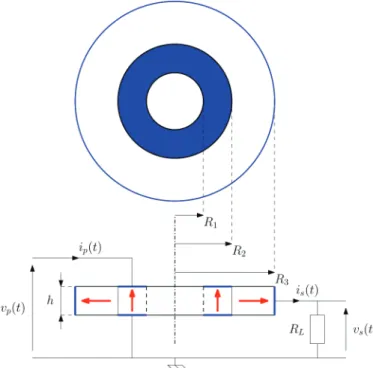
in Fig. 1. The pT is composed of a primary part of inner radius R1 and outer radius R2 poled in the thickness
di-rection and a secondary part radially polarized spreading from the radii R2 to R3. This architecture of thickness h
is driven by an ac voltage power supply applied to the driving section by means of two annular electrodes. at the receiving section, the electric charges generated by the direct piezoelectric effect are gathered on a cylindrical electrode with radius R3 and height h on the outer edge
of the ring. Thereafter, the cylindrical coordinate system is chosen and its origin is put at the center of the trans-former.
2) Mechanical Hypothesis: M1: Because the optimum
performance of this structure is achieved for radial modes, the pT is considered as a thin hollow cylinder whose first radial modes are taken into account. This assumption needs to respect (h ≪ R3).
M2: a purely radial displacement assumption requires that the orthoradial displacement is negligible. Further-more, the radial component of the displacement is sup-posed to be independent of the θ− and z− coordinates due to the axisymmetry and low thickness. as a consequence, the following relationships are supposed to be verified:
uθ = 0 and u r z tr( , , , ) =θ u r tr( , ). (1) M3: The assumption of a plane stress motion is put forward. The normal stress, Tzz, and the shear stresses,
Tτz and Tθz, are consequently assumed to be zero. The last shear stress Tτθ is vanished due to the axisymmetry in such a way that
Tzz =Tθz =Trz =Trθ = 0. (2)
M4: The pT is supposed to be traction-free on its inner and outer edges, leading to the following conditions:
T rrr( =R t1, ) = 0 and T rrr( =R t3, ) = 0. (3)
3) Electrical Hypothesis: E1: The primary part being
assumed reasonably thin and supplied from its lower and upper faces, the electric field E, deriving from the electric potential ϕ, is supposed to be only orientated along the
z-axis leading to:
E = 0 0[ −φ,z] ,T (4)
where (.),z denotes a partial derivative with respect to the
variable z and a superscripted T indicates matrix trans-position.
E2: The primary side is supposed to be respectively connected to the potential vp(t) and the ground on its
lower and upper faces so much that
∀ ∈ =
− =
{
r [ , ] ,R R1 2 φφ( , =( , =r zr z h/h2, )/2, )tt v tp0( ). (5)
E3: as the secondary part is radially polarized, and besides, it is not electroded on its lower and upper faces, it is supposed that the electric displacement field D is purely radial as follows:
D =[Dr 0 0] .T (6) E4: The secondary part is supposed to be connected to a load resistance Rl so much that
∀ ∈ −z [ h/2, 2] , ( =h/ φr R z t3, , ) = ( ) =v ts R i tL s( ), (7)
where vs and is are the voltage at the terminals of the load resistance and the current through it, respectively.
B. Constitutive Relationships
1) Driving Section: as the primary part behaves like an
actuator, the set of two independent variables (S, E) is consequently chosen. These general constitutive relation-ships are reminded in [17, ch. 2, sec. 8, p. 51, eq. 2.8–5] where the material matrices are expressed in accordance with the axial polarization of the primary section. The application of the hypothesis M2, M3, and E1 on these constitutive relationships leads to
T c u c u r e E T c u c u r e E D e rr E r r E r z E r r E r z z = + − = + − = 11 , 12 31 12 , 11 31 / / θθ 331 ,ur r +e u r31 r/ +ε33SEz, (8)
where the strain-displacement relationships Srr = ur,r and
Sθθ = ur/r have been used. The bar symbol on the mate-rial coefficients is a note to use the specific value of the radial transverse coupling mode. These coefficients are
given in Table I, where σ12E and kp are the poisson’s ratio
at constant electric field and the material coupling factor relative to the radial transverse mode, respectively.
2) Receiving Section: as the secondary part behaves
like a sensor, the set of two independent variables (S, D) is consequently chosen. as reminded in [17, ch. 2, sec. 8, p. 51, eq. 2.8–10] and according to M2, M3, and E2, the constitutive relationships are reduced to the following ex-pression: T c u c u r h D T c u c u r h D rr D r r D r r D r r D r r r = + − = + − = 33 , 13 33 13 , 11 31 , / / θθ φ hh u33 ,r r+h u r31 r/ −βS33Dr. (9)
The bar symbol on the material coefficients is a note to use the specific value of the radial longitudinal coupling mode. These coefficients are given in Table II, where σ13E is the poisson’s ratio at constant electric field relative to the radial longitudinal mode.
C. Determination of Electrical Quantities
1) Electric Field in the Primary Part: For the driving
section, the electric displacement field is given by the fol-lowing relationship:
Dz e ur r e u rr S z
= 31 , + 31 / −ε φ .33 , (10)
In fact, it results from the Gauss’s law verified throughout piezoelectric material:
Dz z, = 0⇔φ,zz = 0⇔φ( , ) =z t A t zφ( ) +B tφ( ), (11)
where Aϕ and Bϕ are two constants of integration func-tion of the time t. They can be determined from E2 so much that the electric potential in the driving section is expressed as follows:
φ( , ) =z t v tph( )
(
z +2h)
, (12)and the z-axis component of the electric field is
E tz( ) =−v tph( ). (13)
2) Electric Displacement Field in the Secondary Part:
For the receiving section, the electric displacement field is given from the Gauss’s law verified throughout piezoelec-tric material by D r D D r t C t r r r, r r S 33 1 = 0 ( , ) = ( ) + ⇔ φ β , (14)
where Cϕ is a constant of integration function of the time
t. The latter can be determined from the quantity of
elec-tric charges qs gathered on the edge of the secondary sec-tion defined as follows:
q t D r R t R z h h r s / / d d ( ) = ( = , ) 0 2 2 2 3 3 −
∫ ∫
− π θ ( ) , (15) so much that D r tr( , ) =−2q tπs( )rh. (16)D. Lagrangian of the Piezoelectric Transformer
The lagrangian L of the studied system is the sum of two contributions corresponding to the primary and sec-ondary parts so much that
L=Lp+ .Ls (17) Each term of the previous relationship is classically de-fined by the difference of a kinetic coenergy T * and a
po-TaBlE I. piezoelectric Material coefficients of the radial Transverse coupling Mode. c s E E E 11 11 12 2 = 1 1 ( )− σ e d sE E 31 31 11 12 = (1− σ ) σ12 12 11 = E E E s s − c s E E E E 12 12 11 122 = 1 ( ) σ σ − ε33S =εT33(1−kp2) kp=k31 1 2 E 12 − σ
TaBlE II. piezoelectric Material coefficients of the radial longitudinal coupling Mode.
c k s D E 11 33 2 11 =1 − δ h k k k d E 31 31 31 33 13 31 = ( +δ σ ) β σ ε δ 33 13 2 33 =1 ( ) S E T − c k k s s D E E E 13 31 33 13 11 33 = + σ δ h k k k d E 33 33 33 31 13 33 = ( +δ σ ) σ13 13 11 33 = E E E E s s s − c k s D E 33 31 2 33 =1 − δ δ = (1 31)(1 ) ( σ ) 2 332 31 33 13 2 −k −k − k k + E
tential energy U. If there is no ambiguity on the definition of U in a purely mechanical framework, it differs for a piezoelectric system in accordance with the function, ac-tuator or sensor, accomplished by this one. It can be summed up in the following way:
• primary part = actuator: To study such a behavior, the independent variable set (S, E) has been chosen (see section II-B). The potential energy U thus identi-fies with a free enthalpy G2a so much that the lagrang-ian of the primary part is written as follows [18, ch. 2, sec. 2.5.2, p. 16, Table 2.1]: Lp p T T T T T p d =12 [ [ ] 2 [ ] [ ] ] Ω Ω
∫
ρ u u −S cES+ S e E+E εSE , (18) where ρp and Ωp are, respectively, the mass density and the volume of the primary section. This conven-tion goes hand in hand with a displacement/flux link-age formulation based on the use of the generalized coordinates and velocities (u, λp) and ( , ) u vp, respec-tively. The expression (18) can be made explicit by using the strain-displacement relationships and the electric field Ez in the driving section given by (13)leading to expression (22). The clamped capacitance of the driving section has been defined with the fol-lowing expression: C S R h R p= 33 ( 2 ) 2 12 ε π − . (19)
• secondary part = sensor: For this function accom-plished by the secondary section, the independent variable set (S, D) has been chosen (see section II-B). The potential energy U thus identifies with a free en-ergy Fs so much that the lagrangian of the second-ary part is written as follows [18, ch. 2, sec. 2.5.2, p. 16, Table 2.1]: Ls s T T T T T s d = 12 [ [ ] 2 [ ] [ ] ] Ω Ω
∫
ρu u −S cDS+ S h D D− βSD , (20) where ρs and Ωs are the mass density and the volume of the receiving part, respectively. This convention goes hand in hand with a displacement/charge formu-lation based on the use of the generalized coordinates and velocities (u, qs) and ( , ) u is, respectively. The ex-pression (20) can be made explicit by using the strain-displacement relationships and the electric displace-ment field Dr in the receiving section given by (16) leading to the expression (23) with ν = (c11D/c33D)1 2/and σ13D =c13D/c33D. The clamped capacitance of the
receiving section has been introduced by means of the following relationship: C h R R S s / = 2 33 3 2 π β log( ), (21) Lp= 12 p 2 1 1 2 2 11 , 2 12 , R R r E r r r E r r r u c u ur u ur
∫
− (
+)
−(
−)
ρ σ − + + 2e31 ur r, urr vhp (2πrh r)d 21C vp p2, (22) Ls =12 s r 2 2 3 2 33 , 2 13 , R R D r r r D r r r u c u ur u ur∫
− + −(
−)
ρ ν ν σ − + − 2 h u33 ,r r h31urr 2πqrhs (2πrh r)d 21Cqqs s 2 . (23)E. Application of Hamilton’s Principle
according to [19], a general form of Hamilton’s prin-ciple applied to a pT is t t t i f extd
∫
(δL+δW ) = 0, (24) where δL and δWext are the variations of the pT’s la-grangian and the work done by external sources and forc-es on the time interval [ti, tf], respectively. The latter is expressed as follows:δWext( ) = ( )t i tp δλp( )t +f t q tR( ) ( )δ s , (25)
with f tR( ) symbolizing a damping force, due to the Joule’s first law in the load resistance, expressed by [20, ch. 3, sec. 3.4.3, p. 74, eq. 3.47],
f tR R q tqs s
( ) =−∂∂( , ) , (26)
where R q t( , ) s , named the rayleigh dissipation function, is defined by [20, ch. 3, sec. 3.4.3, p. 74, eq. 3.49],
R q t( , ) = 12R q tL 2( )
s s . (27)
In the previous relationship, the load resistance Rl plays the role of a dissipation constant linked with the general-ized velocity q s. The system configuration is besides sup-posed to be known at initial and final times, so that
∀ ∈ = = r R R u r t u r t t t q t r r [ , ], ( , ) = ( , ) 0 ( ) = ( ) 0 ( ) = 1 3 δ δ δλ δλ δ δ i f p i p f s i qq ts f( )= .0 (28)
on this basis, by means of integrations by parts on the spatial r and time t variables, the stationary of the definite
integral (24) leads to the equations governing the system dynamic. as a consequence, the equation of motion is ex-pressed for both primary and secondary parts, as follows:
c u r t u r t r R R c u r t E r r D r 11 1 1 2 33 ( , ) ( , ) [ , ] ( , ) B B [ ] ∈ [ ] = = p ρ ρ ν , ssu r t r( , )+h312q tsr h( )2 r ∈[ ,R R2 3] π , , (29) where Bα[ ]f is an operator defined for α ∈R by
Bα[ ]f = f,rr r f1 ,r αr f.
2 2
+ − (30)
as well as the mechanical equation (29), two extra equa-tions, respectively named actuator and sensor equaequa-tions, are deduced from Hamilton’s principle and take the fol-lowing form: i tp( ) =C v tp p ( ) 2− πe ru r t31[ r( , )]RR12, (31) q t C v t R h u r t hr u r t r R r r s s s r d ( )= ( ) ( , ) ( , ) 2 3 33 , 31 − +
∫
. (32)Finally, in order that the problem may be well-defined, (29), (31), and (32) need to be completed with the bound-ary conditions (3) and (7) and the continuity relationships expressed at the junction between the driving and receiv-ing sections as follows:
u rr( =R t2−, ) = u rr( =R t2+, ), (33)
T rrr( =R t2−, ) =T rrr( =R t2+, ), (34)
φ( =r R z t2−, , ) = ( =φr R z t2+, , ). (35)
F. Problem Solving
To solve the problem formulated in the previous sec-tion, following the standard modal expansion method, the radial displacement, solution of (29), can be written as an absolutely convergent series of the eigenfunctions as follows: u r tr u r t n r n n ( , ) = ( ) ( ) =1 ( ) +∞ ∞
∑
η , (36)where u( )rn∞( )r and ηn(t) are respectively the mass normal-ized eigenfunction and the modal coordinate of the free-free pT with an open secondary part for the nth radial mode. Thereafter, the infinite subscript (−∞) will be used to remind this configuration.
1) Determination of Eigenmodes: The determination of
eigenmodes is carried out for a free-free pT with a short-circuited primary part (∀t > 0, ( ) = 0)v tp and an open
sec-ondary part (∀t > 0, ( ) = 0)q ts . assuming that the mechan-ical and electrmechan-ical quantities harmonmechan-ically evolve, which means for the radial displacement that ur(r, t) =
ur∞( )r exp ω(j t) with j2 = −1 and u r
r∞( ) its amplitude at
the angular frequency ω, the mechanical equation (29) is reduced to u r u k r u r R R u r u r rr r r r r rr r ∞ ∞ ∞ ∞ ∞ + + − = ∈ + , , 12 2 1 2 , , 1 1 0 [ , ] 1 , rr + k −r ur r R R = ∈ 22 ∞ 2 2 0 [ ,2 3] ν , , (37) where k1 and k2 are, respectively, the wave vectors within the primary and secondary parts whose expressions are
k cE sE E 1 11 11 12 2 =ω ρp =ω ρ 1 ( )σ p − , (38) k cD sE k 2 33 33 31 2 =ω ρs =ω ρs δ/ −(1 ); (39)
ur∞ is thus the solution of a classical homogeneous Bes-sel’s equation of order 1 and v on the primary and second-ary parts, respectively, so much that
ur r C J k rA J k ru B Y k rD Y k ru rr R R u u ∞( ) = 1 1( )( )++ 1 1( )( ) ∈∈[ , ]1 2 2 2 , , ν ν [[ ,R R2 3]
{
, (40)where (J1, Jν) and (Y1, Yν) are Bessel functions of the first
and second kinds of orders 1 and ν, respectively. Au, Bu,
Cu, and Du are constants of integration. Then, the
expres-sion of the electric potential can be obtained by injecting the part of (40) relative to the receiving section into the third equation of the constitutive relationship (9) and then integrating. Knowing that the primary part is short circuited, the electric potential φ∞ associated to the mod-al radimod-al displacement ur∞ is only nonzero on the receiving section with the following expression:
φ∞( ) =r h C J33[ u −( )h1,ν( )k r2 +D Yu −( )h1,ν( )]k r2 +Dφ, (41)
where the function Cµ ν( )h,, defined by (42), and the identity (43) [21, ch. X, sec. 10.74, p. 350, eq. 5] have been used with C being able to be equally substituted by J or Y in both relationships. ∀ ∈z z z +h
∫
h z z z h R, ( ),( ) = ( ) 31 ( ) 33 Cµ ν Cν µCν d . (42)It has to be noted that sµ,v(z) symbolizes in the expression (43) the lommel function of the first kind whose expres-sion can be found in [21, ch. X, sec. 10.7, p. 346, eq. 10]. This function is a particular solution of a lommel’s differ-ential equation (i.e., a nonhomogeneous Bessel’s equation with a power function as the right-hand side):
∀ ∈ ± ∉ − − ∈ + − −
∫
− − z n n z z z z z s z R, { 2 1; N}, ( ) = ( 1) ( ) 1, 1( ) µ ν µ ν µ ν ν µ ν C d [ C CCν−1( )z sµ ν,( )z ]. (43) In fact, it remains to determine five constants of integra-tion (Au, Bu, Cu, Du, Dϕ) and the resonant angularfre-quency ω of the considered structure. To solve this prob-lem, the boundary conditions (3) and the continuity relationships (33) to (35) have been used. The radial com-ponent of the stress tensor Trr is deduced from the expres-sion (40) inserted into the first equations of the constitu-tive relationships (8) and (9) so that
T r c k A J k r B Y k r r R R c k C J rr E u E u E D u D ( ) = 11 1 1( )1 1 ( )1 [ , ]1 2 33 2 [ ], [ + ∈ ν(( )k r2 +D Y k ru D( )2 r ∈[ ,R R2 3] ν ], , (44) The Bessel’s functions in (44) can be expressed by the generic forms C1E and CνD(C being able to be equally
sub-stituted by J or Y) as follows: C C C C C C 1 0 12 1 1 13 ( ) ( ) 1 ( ) ( ) ( ) ( ) E E D D ξ ξ σ ξ ξ ξ ξ ν ξ ξ ν ν ν = − − = − − −σ . (45)
combining (40), (41), and (44) with the relationships (3) and (33) to (35), the following singular system is obtained:
M∞ ( ) = 0 0 0 0 0 ω φ A B C D D u u u u , (46)
where M∞( )ω is a 5 × 5 matrix function of ω. The reso-nant angular frequency ω∞( )n is the nth root of the secular
equation det[M∞( )] = 0ω , which is explicitly given by (47)
where ξij( )n =k Ri( )n j
∞ for ( , ) 1;2 1;3i j ∈ × . The nth mechani-cal mode shape ur( )n∞( )r and electric potential φ∞( )n( )r are defined, for instance, by expressing (Bu, Cu, Du, Dϕ) as a function of the remaining constant of integration Au using (46) removed one line. The general solution of the pro-posed eigenvalue problem consequently takes the form given by the equations (49) and (50) where
U n A YE n
∞( ) = u/ 1 (ξ ,11( )) Φ( )∞n =h U ,33 ∞( )n and α∞( )n is defined by (47), (48), (49), and (50), see above.
2) Orthogonality of Eigenmodes: Knowing that the nth
mode shape verifies the spatial equation expressed on both primary and secondary parts as follows:
c u r u r r R R c u E n n rn D r 11 1 ( ) ( ) 2 ( ) 1 2 33 ( ) ( ) 0 [ , ] B B [ ] [ ] , [ ∞ ∞ ∞ ∞ +ρ ω = ∈ ν p (( ) ( ) 2 ( ) 2 3 ( ) ( ) 0 [ , ] n n rn r]+ [ ]u r = , r ∈ R R , ρ ωs ∞ ∞ (51)
the multiplication of the previous equation by the mth mode shape ur( )m∞( )r and an integration over the domain gives the relationship (52),
[ω∞] + ∞ [ ∞ ] π +
∫
( ) 2 ( , ) 1 2 ( ) 11 1 ( ) ( ) ( )(2 ) 2 n n m R R rm E rn R R M u r c B u r rh rd 33 ( ) 33 ( ) ( ) ( )(2 ) = 0∫
urm∞r cDBν[urn∞r ] πrh rd . (52) where M( , )n m =M( , )n m M( , )n mp + s with Mp( , )n m and Ms( , )n m the modal masses of the primary and secondary parts for the
nth mode shape projected on the mth one, respectively,
whose expressions are
[JE n YE n JE nYE n ][JD n 1(ξ11( )) (1 ξ12( ))− 1(ξ12( )) (1 ξ11( )) ν(ξ23( ))) ( ) ( ) ( ) ( ) ( ) 22( ) 22( ) 23( ) 1 11( ) 1 12( ) Y J Y J Y n n D n E n n ν ν ν ξ ξ ξ ξ ξ − − ] [ JJ nYE n JD nYD n JD n 1 12(ξ( )) (1 ξ11( ))][ ν(ξ23( )) (ν ξ22( ))− ν(ξ22( ))YY c c D n D E ν(ξ ) = 23 ( ) 33 11 ] , (47) α∞( ) 11 ξ ξ − ξ ξ 33 1 11( ) 1 12( ) 1 12( ) 1 11( ) = ( ) ( ) ( ) ( n E D E n E n E n E n c c J Y J Y )) ( 23( )) ( 22( )) ( 22( )) ( 23( )) JD nYD n JD n YD n ν ξ ν ξ − ν ξ ν ξ , (48) urn r U n YE n J k rn JE nY kn ∞ ∞ ∞ − ∞ ( )( ) = ( ) 1 (ξ11( )) (1 1( ) ) 1(ξ11( )) (1 1( )rr Y J k r J Y k r n D( n) ( n ) D( n) () n ) ( ) 23( ) 2( ) 23( ) 2( ) , [ ], α∞ ν ξ ν ∞ − ν ξ ν ∞ ∈ ∈ r R R r [ ,[ , ]R R12 23], (49) φ α ν ξ ν ∞ ∞ ∞ − ∞ ∈ ( ) ( ) 1 2 ( ) 23 ( ) 1, ( ) 2( ) ( ) = 0 [ ( )[ ( [ , ] n n n D n h n r Φ , Y J k rr J) h ( n)] JD( n)[Y h (k r Yn ) r R R 1, ( ) 22( ) 23( ) ( )1, 2( ) (1, − − ν ξ − ν ξ − ν ∞ − −hh)ν(ξ22( )n)]], r ∈[ ,R R2 3]. (50)
M n m u r u r rh r R R rm rn p( , )= ( )( ) p ( )( )(2 )d 1 2
∫
∞ ρ ∞ π , (53) M n m u r u r rh r R R rm rn s s d ( , ) = ( )( ) ( )( )(2 ) 2 3∫
∞ ρ ∞ π . (54) Furthermore, the second part of the expression (52) can be rewritten by considering on the appropriate interval the following identities:c u r c u r T r r T E rn D rn rr r n 11 1 ( ) 33 ( ) , ( ) ( ) ( ) = ( ) 1 B B [ ] [ ∞∞ ] [ + ν rrr n r T rn ( )( )− ( )( ) θθ ]. (55)
as a consequence, an integration by parts on the space variable r and the use of the boundary conditions (3) and the continuity relationship (34) lead to a simplification of (52) so much that
[ω∞( ) 2n]M( , )n m −K( , )n m = 0, (56)
where K( , )n m =K( , )n m K( , )n m
p + s with Kp( , )n m and Ks( , )n m the modal stiffnesses of the primary and secondary parts for the nth mode projected on the mth one, respectively. Their expressions are specified by the relationships (57) and (58). To show the orthogonality condition, the same procedure can be applied for the mth mode leading to
K n m c u r r u r u R R E r rm E rm r rn p( , )= 11 ( ),( ) 12 ( )( ) ( , 1 2
∫
∞ + ∞ ∞ σ )) 12 ( ) 122 2 ( ) ( ( ) ( ) 1 ( ) r r u r r u r u E rn E rm rn + + − ∞ ∞ ∞ σ σ ( ) ))( ) (2r rh r) π d , (57) K n m c u r r u r u R R D r rm D rm r rn s( , )= 33 ( ),( ) 13 ( )( ) ( , 2 3∫
∞ + ∞ ∞ σ )) 13 ( ) 2 13 2 2 ( ) ( ( ) ( ) ( ) r r u r r u r u D rn D rm r + + −( )
∞ ∞ ∞ σ ν σ nn)( ) (2r rh r) π d , (58) [ω∞( ) 2m]M( , )m n −K( , )m n = 0. (59)Finally, by subtracting (59) from (56) and recalling that m and n are distinct modes (ω( ) ω( ))
∞m ≠ ∞n , the symmetry of the modal mass and stiffness matrices [see the expressions (53) and (54), then (57) and (58)] enables to highlight the orthogonality condition of the eigenfunctions so much that
∀ ∈ ∞ ( , ) ( ) , = = * 2 ( , ) ( , ) ( ) 2 m n M K m n nm m n nm m N δ δ ω , (60)
where δnm is the Kronecker’s delta. By assuming that the pT is composed of the same material for the driving and receiving sections, which means ρp = ρs = ρ, the mode shapes can be normalized according to the modal mass normalization criterion (60) defined for this cylindrical structure by ∀ ∈n
∫
u ∞r rh r R R rn N*, [ ( )( )] (22 ) = 1 1 3 ρ π d . (61)It enables determination of the constant U n
∞( ) given by (64) where the expression (40) giving the modal radial dis-placement, to simplify the calculus, has been rewritten as follows: urn r U n rr rr R RR R ∞ ∞
{
∈∈ ( ) ( ) 1,1 1 2 2, 2 3 ( ) = CC ( )( ),, [ ,[ , ]], ν (62) with Cα β, ( )r defined by Cα β, ( ) =r A J k rα β α( ( )n∞)+B Y k rα β α( ( )n∞), (63) and by identification A YE n 1 = 1 (ξ ,11( )) B1 =−J1E(ξ ,11( )n) A2 = α∞( )nYνD(ξ23( )n), and B2 =−α( )∞n DJν(ξ23( )n). U n h r r r r r r R R ∞( )= ρπ ([ [2C1,12( )−C1,0( )C1,2( )]] 12 +[ [2C2,2ν( ) −C2, −1 C2, +1 23 − 1/2 ( ) ( )]] ) ν r ν r RR . (64)3) Response to a Harmonic Supply Voltage: In this
sec-tion, the pT is supposed to be supplied by a harmonic input voltage vp(t) = Vpcos(ωt). The solution of the
me-chanical equation (29) to this excitation can be expressed by means of (36) and the orthogonality condition (60) relative to the chosen eigenfunctions. To perform this, both equations of the equation of motion (29) are multi-plied by the mass-normalized mode shape ur( )m∞( )r and inte-grated over the primary and secondary sides, respectively. The result is shown by (65):
n n m n R R rm E rn M t u r c u r =1 ( , ) ( ) 11 1 ( ) ( ) ( ) ( )(2 1 2 +∞ ∞ ∞
∑
−∫
{
η B [ ] ππ π η ν rh r u r c u r rh r t R R rm D rn n ) ( ) ( )(2 ) ( ) 2 3 ( ) 33 ( ) d d + }
∫
∞ B [ ∞ ] = = ( ) ( ) 2 3 31 ( ) −q ts∫
hr u ∞r r R R rm d . (65) Then, by using the identity (55) and an integration by parts on the space variable r, the ηnt()-coefficient in (65) can be simplified by the following quantity:−K n m + ru ∞r T r rm rrn RR ( , ) ( ) ( ) 1 3 ( ) ( ) [ ] . (66)
Finally, by invoking the orthogonality condition (60) and using the boundary conditions (3) and the continuity of the radial stress (34), it results an infinite system of me-chanical equations as follows:
∀ ∈n nt + ∞n t ∞v t − ∞q t
n pn p sn s
where ψp( )n∞ and χ
s( )n∞ are the electromechanical coupling factors within the primary and secondary sides for the nth mode shape. ∀ ∈n N*,ψp( )n∞= 2− πe U R31 ( )∞n[ 2 1,1C ( )R2 −R1 1,1C ( )]R1 , (68) ∀ ∈ = [ + [ − − ∞ ∞ − − n N*,χs( )n U( )n h33 2,C ν( )ξ h31ξ ν( 2)C2,ν( )ξs 2,ν 1( )ξ CC2, 1( ) 1,( ) 22 ( ) 23 ( ) ν− ξs− νξ ]]ξξn n . (69) The previous equation can be expressed in function of the secondary voltage vs(t) by using the sensor equation (32)
so much that the equations governing the electrodynami-cal behavior of the pT are obtained and can be summa-rized in (70), see above, where the relationship ψs( )n∞=Cs sχ( )n∞ has been used. Moreover, a modal mechanical quality fac-tor Qm( )n has been added in the mechanical equation in
(70), which will be able to be experimentally deduced or arbitrarily set. It has to be noticed that the radial modes are coupled by crossed terms that can be interpreted as an extra stiffness in the mechanical equation. The system of (70) is uncoupled for an open circuit condition (qs = 0), in
accordance with the chosen modal basis, in such a way that for n ∈ N*: ηn ωn η ω η ψ mn n n n pn t Q t t v t i t ( ) ( ) ( ) = ( ), ( ) ( ) ( ) ( ) 2 ( ) + ∞ + ∞ ∞ p p == ( ) ( ), ( ) = ( ). =1 ( ) =1 ( ) C v t t t C v t r r r r r r p p p s s s + +∞ ∞ +∞ ∞
∑
∑
ψ η ψ η (71)It is possible to give the expression of the input admit-tance Yp∞=i vp/ p from the actuator and the mechanical equations in (71) so much that
Y j C C X jX Q p p n mn mn ∞ +∞ ∞ + − +
∑
( ) = 1 =1 ( ) 2 ( ) ω ω / , (72) where X =ω ω/ ( )n∞ is a dimensionless angular frequency and Cmn n n
∞ ∞ ∞ ( ) = ψ( ) ω( ) 2
p / is the motional capacitance of the
nth radial mode. Thereafter, putting this method into
practice will need to truncate the modal basis to a few modes, for instance N. The required quantities to obtain this model are consequently:
• the first N resonant angular frequencies ( ( ))
1,
ω∞n n∈ N,
mode shapes (u( )rn∞ ∈)n 1,N and mechanical quality
fac-tors ( ( ))
1,
Qmn
n∈ N for an open ring rosen-type pT,
• the first N electromechanical coupling factors
( ( ))
1,
ψp∞ ∈n n N and (χ( )s∞ ∈n)n 1,N of the primary and
second-ary parts,
• the input and output clamped capacitances Cp and
Cs.
III. numerical and Experimental Validation To validate the relevance of the previously developed analytical modeling, numerical simulations and experi-mental characterizations were carried out. The numerical study takes advantage of a finite element method using the ansys software. a 2-d study assuming plane stress motion has effectively enabled to plot the mechanical mode shapes and the distribution of the electric potential along a radius of the considered structure. regarding the experimental validation, this one is based on admittance measurements with an impedance analyzer (agilent Tech-nologies, Hp4294a). This validation has been undertaken on four samples, named (s1) to (s4), composed of the pZT-type material apc841. all the pTs have the same dimensions, their differentiation only relying on a differ-ent intermediate radius, R2 from 10 mm (s1) to 13 mm (s4). The geometrical and structural parameters of these pTs are itemized in Table III, where ε0 = 8.854 × 10⁻¹²
symbolizes the vacuum permittivity.
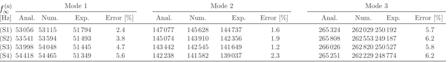
First of all, the Table IV allows to compare the reso-nant frequencies of a ring rosen-type pT with an open secondary part for the first three radial modes and for the four considered samples. The results from the analyti-cal modeling, the numerianalyti-cal simulation and experimental measurements are very satisfactory, as confirmed by the percent error between the theoretical and experimental values (see Error [%] in Table IV). However, it has to be noticed that this error increases with the mode rank. It is due to the initial assumptions, essentially M1, M2, and M3. ∀ ∈ + ∞ + − ∞ ∞ +∞
∑
n t Q t t n n mn n n n sn r N* ( ) ( ) ( ) 2 ( ) =1 , ( )η ω η ( ) [ω ]η ( ) χ ψssr r pn p sn s p t v t v t i t ∞ = ∞ − ∞ = ( ) ( ) ( ) ( ) ( ) ( ) ( ) η ψ ψ (mechanical eq.), C C v tp p t r p r r r s r r ( ) ( ) =1 ( ) =1 ( ) + +∞ ∞ +∞ ∞∑
∑
ψ η ψ η (actuator eq.), (( )t =C v ts s ( )+i ts( ) (sensor eq.), (70)additionally, the measurements of the input admit-tance and its theoretical evaluation by the expression (72) are presented on a wide frequency range. For readability reasons, only experimental and theoretical results of sam-ples (s1) and (s4) are presented, in Figs. 2(a) and 2(b), respectively. amplitude and phase are plotted on the same graph for qualitative comparison between modeling and measurements. The computation of the formula (72) has been performed for the first N = 100 radial modes. The modal mechanical quality factors Qn
m( ) have been identified with their experimental values for the first three modes and set to the material value for the remaining modal quantities. The accuracy is quite satisfying with an error increasing with the mode rank, even with a greater num-ber N of radial mode shapes considered for the computa-tion. It is a typical limitation of the initial assumptions when mechanical wavelength is reduced. It tends to dem-onstrate that the range of interest for this modeling is limited to the rank of first modes. another origin of dis-crepancy between theory and experiment may be the po-larization process which does not necessarily ensure a per-fect radially polarized secondary part. Indeed, to polarize the receiving part, a constant potential difference is ap-plied between the intermediate radius R2 and the outer
radius R3. as a consequence, because of the cylindrical
geometry, a spatially variable electric field (∝ 1/r) is in-duced.
despite this observed disparity, the theoretical ap-proach enables to thoroughly study the influence of the
geometric parameters in view of a pT’s design dedicated to a specific application. For instance, within the frame-work of the plasma generation obtained by piezoelectric sources (see [22] for more details), it is obvious that the electric potential and its distribution are essential crite-ria for the promotion of ac plasma discharges. Indeed, the plasma discharge is strongly dependent on the electric field in the gas surrounding the transformer. The voltage value obtained on the surface and more particularly at the edge of the ring can be the local origin of the ignition and the sustainability of the discharge. It is consequently function of the radial mode.
Fig. 3 shows the normalized electric potential distribu-tion on the ring surface along the radius for the first four radial modes. parametric influence of the intermediate ra-dius R2 is also illustrated in accordance with existing
sam-ples (s1) to (s4). It has to be noted that the developed model also gives the opportunity to draw the normalized radial displacement from (40). although the curves in Fig. 3 do not inform about the absolute voltage value (normal-ized curves), it is possible to discuss the different modes.
among the four modes, the second and the fourth are particularly interesting. The former reaches the maximum voltage at the edge of the ring. Thus, the electric field in the gas immediately surrounding the edge could be very high. as a consequence, the plasma discharge may appear at the edge, all around the ring. additionally, the fourth mode presents two optimum values, positive and nega-tive. This configuration gives the opportunity to reach
TaBlE III. Material properties of apc841 ceramic and Geometric parameters of ring rosen-Type pTs.
definition Value Unity
R1 Inner radius 4 mm R2 Intermediate radius [10, 13] mm R3 outer radius 20 mm h Thickness 1 mm ρ Mass density 7652 kg/m3 sE
11 Transversal compliance at constant E 11.7 μm2/n
sE
12 Transversal compliance at constant E −6.3 μm2/n
sE
13 Transversal compliance at constant E −4.2 μm2/n
sE
33 longitudinal compliance at constant E 13.9 μm2/n
d31 Transversal piezoelectric coefficient −100 pm/V
d33 longitudinal piezoelectric coefficient 280 pm/V
εT33 longitudinal permittivity at constant T 1380 ε0 F/m
k31 Transversal coupling factor 0.264
k33 longitudinal coupling factor 0.679
Qm Mechanical quality factor 1300
TaBlE IV. resonant Frequencies of a ring rosen-Type pT With an open secondary side for the First Three radial Mode, samples (s1) to (s4), comparison of the analytical (anal.), numerical (num.), and Experimental (Exp.) results. f n
∞( )
[Hz]
Mode 1 Mode 2 Mode 3
anal. num. Exp. Error [%] anal. num. Exp. Error [%] anal. num. Exp. Error [%]
(s1) 53 056 53 115 51 794 2.4 147 077 145 628 144 737 1.6 265 324 262 029 250 192 5.7
(s2) 53 541 53 594 51 493 3.8 145 074 143 910 142 356 1.9 265 808 262 553 249 187 6.2
(s3) 53 998 54 048 51 445 4.7 143 442 142 545 141 649 1.2 266 026 262 820 250 527 5.8
Fig. 2. Theoretical (solid line) and experimental (dashed line) input admittance (magnitude and phase) for samples (s1) and (s4).
very high electric field on the ring surface, especially in the illustrated configuration (s3). In such configuration, plasma discharge will appear on the ring surface, mainly located between R2 and R3. other modes may also be useful to change the plasma patterns. as a consequence, by cautiously observing Fig. 3, it clearly appears that the intermediate radius and the radial mode shapes can be the subject of a future optimization in view of designing a pT dedicated to plasma generation with a voltage gain as high as possible. Moreover, it has to be noticed that oper-ating frequency is an essential parameter for the piezoelec-tric device as well as for the plasma discharge behavior. Indeed, the step-up voltage is only efficient close to one of the resonance frequencies of the transformer. likewise, the produced ac electric field may strongly affect the plasma discharges because of the dynamic behavior of the electric charges (sheath formation, ignition, extinction, etc.). as a consequence, specific attention will be paid to the optimi-zation of the resonant frequency and the resulting design of the device.
IV. conclusion
This paper has demonstrated full analytical modeling for a ring rosen-type pT. The application of Hamilton’s principle has enabled establishment of the equations gov-erning the electromechanical behavior of the considered structure. The problem has been solved with the classical modal expansion method, and the case of a pT with an open secondary has been more precisely studied and vali-dated with numerical and experimental results. With the purpose of using this device as plasma discharge genera-tor, one of the essential pieces of information is the electric potential distribution on the surface of the transformer. The results have shown that several vibratory modes are interesting to investigate and to be specifically the target of optimization to increase the electric field. This work has been the first step of an extended study that will include optimization of design, carrying out deterministic methods based on an analytical behavioral model [23], and plasma discharge characterizations.
references
[1] c. a. rosen, K. a. Fish, and H. c. rothenberg, “Electromechanical transducer,” U.s. patent 2 830 274, apr. 8, 1958.
[2] s. Manuspiya, T. Ezaki, B. Koc, and K. Uchino, “laptop adaptor using a piezoelectric transformer—drive circuit development,” in
5th Int. Conf. on Intelligent Materials, penn state, pa, Usa, Jun.
2003.
[3] M. day and B. s. lee, “Understanding piezoelectric transformers in ccFl backlight applications,” Analog Applications Journal, Texas Instruments Incorporated, pp. 18–23, 2002.
[4] G. H. Hufferd, H. l. Vail, Jr., and r. H. Josephson, “Voltage or spark source,” U.s. patent 3 082 333, Mar. 19, 1963.
[5] s. H. newman, “cigarette lighter,” U.s. patent 3 295 024, dec. 27, 1966.
[6] H. Itoh, K. Teranishi, and s. suzuki, “observation of light emissions around a piezoelectric transformer in various gases,” IEEE Trans.
Plasma Sci., vol. 30, no. 1, pp. 124–125, Feb. 2002.
[7] K. Teranishi, d. Inada, n. shimomura, s. suzuki, and H. Itoh, “VUV spectroscopic measurement for dielectric barrier discharge ex-cited by piezoelectric transformer in He-Xe mixture,” IEEE Trans.
Plasma Sci., vol. 36, no. 4, pp. 1340–1341, aug. 2008.
[8] M. Teschke and J. Engemann, “low voltage app-generation by piezo ceramics: Basic structures, electro-mechanical simulations and poling techniques,” in Proc. 18th Int. Symp. Plasma Chemistry, Kyoto, Japan, aug. 26–31, 2007.
[9] H. Kim, a. Brockhaus, and J. Engemann, “atmospheric pressure argon plasma jet using a cylindrical piezoelectric transformer,” Appl.
Phys. Lett., vol. 95, issue 21, art. no. 211501, 2009.
[10] J. Engemann and M. Teschke, “device for producing an atmospher-ic pressure plasma,” U.s. patent 2009/0122941 a1, May 14, 2009. [11] J. s. yang and X. Zhang, “Extensional vibration of a nonuniform
piezoceramic rod and high voltage generation,” Int. J. Appl.
Electro-magn. Mechan., vol. 16, no. 1–2, pp. 29–42, Jan. 2002.
[12] c. nadal and F. pigache, “Multimodal electromechanical model of piezoelectric transformers by Hamilton’s principle,” IEEE Trans.
Ultrason. Ferroelectr. Freq. Control, vol. 56, no. 11, pp. 2530–2543,
nov. 2009.
[13] J. s. yang and X. Zhang, “analysis of a thickness-shear piezoelec-tric transformer,” Int. J. Appl. Electromagn. Mechan., vol. 21, no. 2/2005, pp. 131–141, apr. 2005.
[14] p. půlpán and J. Erhart, “Transformation ratio of ring-dot planar piezoelectric transformer,” Sens. Actuators A, vol. 140, no. 2, pp. 215–224, nov. 2007.
[15] s. lin, J. Hu, and Z. Fu, “Electromechanical characteristics of piezo-electric ceramic transformers in radial vibration composed of con-centric piezoelectric ceramic disk and ring,” Smart Mater. Struct., vol. 22, no. 4, art. no. 045018, Mar. 2013.
[16] W. chen, c. lu, J. yang, and J. Wang, “a circular cylindrical, radi-ally polarized ceramic shell piezoelectric transformer,” IEEE Trans.
Ultrason. Ferroelectr. Freq. Control, vol. 56, no. 6, pp. 1238–1245,
Jun. 2009.
[17] J. s. yang, An Introduction to the Theory of Piezoelectricity. new york, ny, Usa: springer science+Business Media Inc., 2005. [18] T. Ikeda, Fundamentals of Piezoelectricity. new york, ny, Usa:
oxford University press Inc., 1996.
[19] c. nadal, “contribution to the conception and the modeling of piezoelectric transformers dedicated to plasma generation,” Thèse de doctorat, Institut national polytechnique de Toulouse, Toulouse, France, Jul. 2011 (in French).
[20] a. preumont, Mechatronics: Dynamics of Electromechanical and
Piezoelectric Systems. dordrecht, The netherlands: springer-Verlag,
2006.
[21] G. n. Watson, A Treatise on the Theory of Bessel Functions, seaside, or, Usa: Watchmaker publishing, 2008.
[22] T. Martin, F. pigache, c. nadal, and T. callegari, “Experimental analysis of piezoelectric plasma discharge generator,” in IEEE Int.
Ultrasonics Symp., pp. 1–5, dresden, Germany, oct. 7–10, 2012.
[23] F. pigache, F. Messine, and B. nogarede, “optimal design of piezo-electric transformers: a rational approach based on an analytical model and a deterministic global optimization,” IEEE Trans.
Ul-trason. Ferroelectr. Freq. Control, vol. 54, no. 7, pp. 1293–1302, Jul.
2007.
Clément Nadal was born in rennes, France, in 1983. He received an engineer’s degree in electrical engineering and a M.s. degree in 2007 from École nationale supérieure d’Électrotechnique, d’Électronique, d’Informatique, d’Hydraulique et des Télécommunications (EnsEEIHT), Toulouse, France. He received a ph.d. degree in electrical engineering from Institut national polytechnique de Toulouse (InpT) in 2011, for his dissertation regarding analytical piezoelectric device modeling dedicated to plasma generation. He currently oc-cupies a postdoctoral position at IrcIca (Institut de recherche sur les composants logiciels et matériels pour l’Information et la communica-tion avancée), University of lille 1, France, for the design of piezoelec-tric devices used for tactile applications.
François Pigache was born in auchel, France, in 1977. He received a M.s. degree in instrumenta-tion and advanced analysis in 2001, and a ph.d. degree in electrical engineering from the Univer-sity of sciences and Technology, lille, France, in 2005. He joined the laboratoire des plasmas et de la conversion d’Énergie, Toulouse, France, as an associate professor. His research concerns multi-physic modeling, the optimization of piezoelectric transformers, and alternative applications of fer-roelectric materials.
Jiří Erhart received his M.sc. diploma from the Faculty of Mathematics and physics, charles Uni-versity in prague, czech republic, in the field of mathematical physics in 1988 and his ph.d. in the field of condensed matter physics in 1999. He worked at the Institute of physics, academy of sciences of the czech republic during 1990–1993. currently he is working at the Technical Univer-sity of liberec, czech republic. He is head of pi-ezoelectricity research laboratory at the depart-ment of physics. He was promoted to associate professor in 2001 and to full professor in 2012. during 1998–1999 he worked as a research fellow and post-doc in the Materials research lab-oratory at The pennsylvania state University, University park, Usa. In 2003 he was awarded The Matsumae International Foundation fellowship for his research stay at the Tokyo Institute of Technology, Japan. He also worked as a visiting research fellow at the city University in Hong Kong and at the Harbin Institute of Technology, china, for shorter stays dur-ing 2002, 2004, and 2009. prof. Erhart specializes in the field of piezo-electricity and piezoelectric materials, ferroelectric domains and domain engineering, piezoelectric ceramics transformers, resonators, and actua-tors.