Shock-cell noise of supersonic underexpanded jets

HAL Id: hal-02088791

https://hal.archives-ouvertes.fr/hal-02088791

Submitted on 3 Apr 2019

HAL is a multi-disciplinary open access

archive for the deposit and dissemination of

sci-entific research documents, whether they are

pub-lished or not. The documents may come from

teaching and research institutions in France or

abroad, or from public or private research centers.

L’archive ouverte pluridisciplinaire HAL, est

destinée au dépôt et à la diffusion de documents

scientifiques de niveau recherche, publiés ou non,

émanant des établissements d’enseignement et de

recherche français ou étrangers, des laboratoires

publics ou privés.

Shock-cell noise of supersonic underexpanded jets

Carlos Pérez-Arroyo, Guillaume Daviller, Guillaume Puigt, Christophe Airiau

To cite this version:

Carlos Pérez-Arroyo, Guillaume Daviller, Guillaume Puigt, Christophe Airiau. Shock-cell noise of

supersonic underexpanded jets. 50th 3AF International Conference on Applied Aerodynamics, Mar

2015, Toulouse, France. pp.0. �hal-02088791�

Any correspondence concerning this service should be sent to the repository administrator:

staff-oatao@listes-diff.inp-toulouse.fr

This is an author-deposited version published in:

http://oatao.univ-toulouse.fr/

Eprints ID: 18325

O

pen

A

rchive

T

oulouse

A

rchive

O

uverte (

OATAO

)

OATAO is an open access repository that collects the work of Toulouse

researchers and makes it freely available over the web where possible.

To cite this version: Pérez-Arroyo, Carlos and Daviller, Guillaume and

Puigt, Guillaume and Airiau, Christophe

Shock-cell noise of supersonic

underexpanded jets. (2015) In: 50th 3AF International Conference on

SHOCK-CELL NOISE OF SUPERSONIC UNDEREXPANDED JETS

C. Pérez Arroyo (1), G. Daviller (2), G. Puigt (3), C. Airiau (4)

(1)

Centre Européen de Recherche et de Formation Avancée en Calcul Scientifique, 42 Avenue Gaspard Coriolis, 31057 Toulouse Cedex 01, France, Email: cparroyo@cerfacs.fr

(2)

Institut de Mécanique des Fluides de Toulouse, UMR 5502 CNRS/INPT-UPS, Allée du professeur Camille Soula, 31400 Toulouse, France, Email: guillaume.daviller@imft.fr

(3)

Centre Européen de Recherche et de Formation Avancée en Calcul Scientifique, 42 Avenue Gaspard Coriolis, 31057 Toulouse Cedex 01, France, Email: guillaume.puigt@cerfacs.fr

(4)

Institut de Mécanique des Fluides de Toulouse, UMR 5502 CNRS/INPT-UPS, Allée du professeur Camille Soula, 31400 Toulouse, France, Email: christophe.airiau@imft.fr

Shock-cell noise is a particular noise that appears in imperfectly expanded jets. Under these expansion conditions a series of expansions and compressions appear following a shock-cell type structure. The interaction between the vortices developed at the lip of the nozzle and the shock-cells generates what is known as shock-cell noise. This noise has the particularity to be propagated upstream with a higher intensity. This publication will focus on the shock-cell noise generated by an axisymmetric under-expanded 106 Reynolds single jet. The LES computations are carried out using the elsA code developed by ONERA and extended by CERFACS with high-order compact schemes. They are validated against experimental results. The LES simulation is initialized with a RANS solution where the nozzle exit conditions are imposed. Even though no inflow forcing is applied, good agreement is obtained in terms of flow structures and broadband shock-cell noise that is propagated to the farfield by means of the Ffowcs-Williams & Hawkings analogy.

INTRODUCTION

For an aircraft at cruise conditions, the noise perceived in the aft-cabin is mainly due to the turbofan jet. In fact, the secondary stream of a turbofan engine is a cold, supersonic and under-expanded jet. The pressure mismatch between the jet and the ambient air leads to the formation of (diamond-shaped) shock-cells as shown in Fig. 1, which strongly interact with the turbulent structures developing in the mixing layer around the potential core. This interaction process produces intense noise components on top of the turbulent mixing noise, which makes supersonic jets noisier than their subsonic counterparts [1]. The result is a broadband shock-cell associated noise (BBSAN), radiated in the forward direction, that impinges on the aircraft fuselage and it is then transmitted into the cabin.

This work focuses on the LES simulation carried

out with elsA solver of an under-expanded cold 106

Reynolds single jet at perfectly expanded

conditions of Mach 1.15. First the main

characteristics of the solver are presented. Second the procedure for the computations are explained and last, the results are shown and analyzed.

NUMERICAL FORMULATION

The full compressible Navier-Stokes equations in skew-symmetric formulation are solved inside elsA [2] software that is a Finite Volume multi-block structured solver developed by ONERA and extended by CERFACS. The spatial scheme is based on the implicit compact finite difference scheme of 6th order of Lele [3] extended to Finite Volumes by Fosso et al. [4]. The above scheme is stabilized by the compact filter of Visbal & Gaitonde [5] that is also used as an implicit subgrid-scale model for the present LES. Time integration is performed by a six-step third-order Runge-Kutta DRP scheme of Bogey & Bailly [6].

Non-reflective radiative and Navier-Stokes

Characteristic boundary conditions are used [7]. Furthermore, sponge layers & a low-pass filter help the simulation to remove spurious noise reflections near the boundaries of the computational domain. In this high order formulation, the code has been validated on a wide variety of flows of increasing complexity, starting from classical acoustic test cases, up to subsonic jets [8][9].

UNDEREXPANDED JET CONDITIONS

Time-dependent simulations are presented of a contoured convergent nozzle with exit diameter D=38.0mm and a modeled nozzle lip thickness of t=0.125D. The nozzle is operated under-expanded at the stagnation to ambient pressure ratio ps/p∞=2.27. The modeled exit and ambient conditions match those in the experimental set-up of André [10]. The ambient conditions of the air are

temperature T∞=288.15K and pressure

p∞=98.0kPa. This cold air jet has an exit stagnation temperature of 288.15K. The Reynolds number, Re, based on the jet exit diameter is 1.2×106 and the fully expanded jet Mach number is Mj=1.15. The flow at the nozzle exit is mainly axial but some vertical components appear due to the inclined inner shape of the nozzle. In addition, a small co-flow of 0.5m/s is added in order to help the convergence of the results.

The airflow is modeled under ideal gas

assumptions, with specific gas constant

R=287.058J/(kg K) and specific heat ratio γ=1.4.

SIMULATION SETUP AND PROCEDURE

The numerical computation is initialized by a RANS simulation using the Spalart-Allmaras turbulence model [11]. The RANS solution is wall- resolved in the inner and outer sections of the

nozzle with y+<1. Once mesh convergence is achieved and the boundary layer at the exit of the nozzle has good agreement with the experimental results, the LES computation is then initialized from the RANS simulation. The inner part of the nozzle is removed from the LES simulation and the RANS nozzle exit conservative variables are imposed as in [12]. In addition, no inflow forcing is used.

The computational domain, sketched in Fig. 2 used for the LES extends 40 diameters in the axial direction and 7 in the radial direction. Non-reflective boundary conditions of Tam and Dong [13] extended to three dimensions by Bogey and Bailly [14] are used in the exterior inlet as well as in the lateral boundaries. The exit condition is based on the characteristic formulation of Poinsot and Lele [15]. Furthermore, sponge layers are coupled around the domain to attenuate exiting vorticity waves.

Figure 2. LES domain sketch

The mesh consists in a three-dimensional mesh with a butterfly on the center to avoid the

axisymmetric singularity. The mesh has 75×106

cells with (1052×270×256) nodes in the axial, radial and azimuthal directions respectively. The mesh used in the LES simulation near the jet lip line is coarsened in the radial direction with respect to the RANS mesh, meaning that no wall resolution is achieved when the RANS solution is interpolated into the LES mesh. Nevertheless, the boundary layer at the exit of the nozzle is defined by 15 points having a y+≈50. The lip is meshed with 12 uniformly spaced cells. Each shock-cell is resolved within 40 cells in the axial direction and up to 220 cells in the radial direction for the first shock-cells. The axial cell distribution grows within the half diameter with an expansion ratio of 3.2%. Then it is set almost constant until the beginning of the sponge layer where it grows at a rate of 14%. Regarding the quality of the mesh, the minimum orthogonality is 54° and the maximum expansion

ratio achieved is less than 4% (without taking into account the sponge layers).

The simulation ran for 120 non-dimensional time units (t*=tD/c∞) to evacuate the transient phenomena that one obtains with an averaged (RANS) solution. After the transient phase, the simulation runs for 120 non-dimensional time units in order to reach statistically independent results. The farfield sound is obtained by means of the FW-H analogy [16]. The surface used to extrapolate the variables to the farfield is located in a topological surface starting at r=3.5D from the axis and growing with the mesh. The cut-off mesh Strouhal is St≈2. In terms of frequency (St =f D/U), this value is defined as f = c∞/(nΔ), where Δ is the cell size, c∞ the ambient speed of sound and n the number of cells needed to resolve fluctuations with the numerical scheme used. Nonetheless, the acquisition frequency at the FW-H surface has been set to 100 kHz (St = 5) in order to properly represent the effect that the cell size has on the spectra.

The LES simulation has been run in parallel in the cluster BULL B510 (neptune) at CERFACS. The computation took around 720 hours running with 128 CPUS (within 8 nodes).

RESULTS

The following section illustrates the LES results obtained within the last 120 non-dimensional time units.

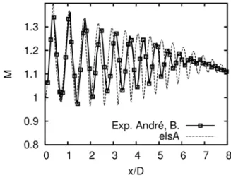
Shock cell noise frequency is proportionally influenced by the size of the shock-cells and their interaction with the most energetic turbulent scales from the first Kelvin-Helmholtz instability. The averaged Mach profile is shown in Fig. 3. Good agreement is obtained for the shock-cell spacing in the first three shock-cells. Even though further downstream, a shift appears between the experimental and the numerical result, the shock-cell spacing is only reduced by 5%. From preliminary analyses, there is a strong confidence that an increase of 50% on the total number of nodes should be sufficient to correctly capture all the shock patterns. Even though the amplitudes are higher than in the experimental results, they follow the same decay having the end of the potential core at the same position.

Another important factor when simulating jets is their expansion rate. The axial velocity profile along the radius at x/D=0.16 is shown in Fig. 4. Good agreement is obtained within the first 3

diameters. Further downstream, the shift in the shock-cells makes the comparison not viable.

Figure 3. Mach profile at the axis

Although no inflow forcing is applied, matching the jet exit profile against the experimental results and a good discretization of the flow, seems to be sufficient for this supersonic jet to transition to a fully turbulent flow within the first radius from the exit nozzle plane. To support this statement, the turbulence levels of the velocity components at the lip line are shown in Fig. 5. As the conditions at the nozzle exit are imposed, it is obvious that the flow starts completely laminar (therefore, the turbulence is zero). However, after the first radius, it has reached the same levels of rms as in the experimental results even though an overshoot is contemplated within the first 2 diameters.

Figure 4. Axial velocity along the radius at x/D=0.16

The size of the turbulent structures generated along the lip line (r/D=0.5) is measured by means of a spatial auto-correlation following the same

Figure 5. Turbulence levels of the axial and radial component of velocity at r/D=0.5

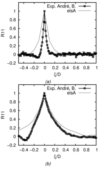
formulation as in [17]. The axial velocity auto-correlations R11 are shown at the positions x/D=1.5 and x/D=9.0 in Fig. 6 (a) and (b) respectively. For this purpose, the computational flow field was probed every 0.1 diameters. The increase in the size of the turbulence structures in the mixing layer is clearly illustrated. The turbulence length scale computed from the auto-correlations along the lip line is shown in Fig. 7. The integration of R11 is done up to the value 0.1. Despite the fact that Fig. 6 (a) and (b) show an increase in size of the turbulence structures with respect to the experimental results, Fig. 7 shows that it presents the same growth rate, but advanced 1.5 diameters in the axial direction. This displacement is probably due to the imposed laminar conditions at the exit of the nozzle, where the transition occurs in a more abrupt fashion as seen in Fig. 5.

The pressure perturbation is measured in two arrays of numerical probes, first with an inclination of 5° from x/D=0.0, r/D=1.0 and second, horizontally at r/D=3.0. The results are plotted in Fig. 8 (a) and (b) respectively. Two distinct patterns are clearly distinguished. The shock-cell noise that propagates upstream becomes apparent at x/D<10.0. On the other hand, the mixing noise produced from the large structures appears in the other region of the flow. The region in between, which is where the potential core ends, generates both types of noises. The results obtained closer to the jet shown in Fig. 8 (a) are clearly biased by the

hydrodynamic fluctuations of the jet. A

hydrodynamic/acoustic filter will be carried out in the future in order to properly separate the hydrodynamic component from the acoustic component that will help analyze the results.

(a)

(b)

Figure 6. Axial velocity autocorrelation at r/D=0.5 and (a) ) x/D=1.5 and (b) x/D=9.0 and

Figure 7. Axial velocity length scale at r/D=0.5 The temporal correlation of the pressure perturbation between the two arrays is done for several positions of the array at r/D=3.0. Fig. 9 (a) and (b) show the correlation at x/D=0.0 and

x/D=10.0 respectively. The BBSAN component of shock-cell noise is usually generated downstream the 5th shock-cell as explained in [18]. The maximal correlation when measuring at x/D=0.0 shown in Fig. 9 (a) is achieved around x/D=4.0. This position corresponds to the 4th – 5th shock-cell. Fig. 9 (b) shows that the perturbations that reach the location at x/D=10.0 are highly correlated at the same location near the jet.

(a)

(b)

Figure 8. Pressure perturbation contours [Pa] along (a) the line at 5° from x/D=0.0, r/D=1.0 and

(b) axial direction at r/D=3.0

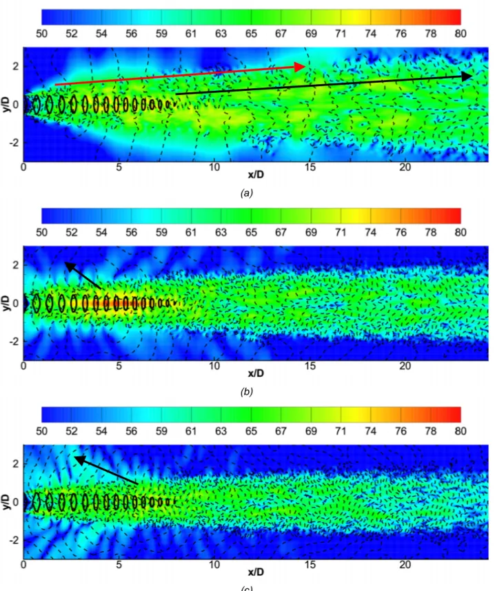
The discrete Fourier transform (DFT) of the pressure can be computed in a two-dimensional plane at z=0. The modulus of the DFT shows where the pressure perturbations are more intense in the flow field. On the other hand, the phase of the DFT gives a visual interpretation of the directivity of the noise. The results are shown in Fig. 10, for different Strouhal numbers. At low Strouhal (Fig. 10 (a)), the energy is intense at the extremes of the shock-cells and two main

downstream directivities can be appreciated. One appears at the exit of the nozzle due to the Kelvin-Helmholtz instabilities (red arrow), and the second one is displayed at the end of the potential core (black arrow). When the frequency is increased (Fig. 10 (b)), the shock-cell noise and its upstream directivity start to appear. For St=0.59, the main source is found at x=4, or at the 6th shock-cell. Higher Strouhal numbers (Fig. 10 (c)) move the source downstream up to x=7 (12th shock-cell).

(a)

(b)

Figure. 9. Temporal correlation of the pressure perturbation between the inclined array at 5° and (a) the probe at x/D=0.0, r/D=3.0 and (b) x/D=10.0,

r/D=3.0

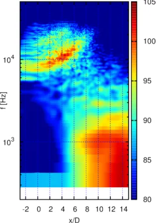
The nearfield sound pressure level (SPL) computed at the horizontal array at y/D=3.0 is shown in Fig. 11. The noise generated from the large structures appears for low frequencies at x>6. On the opposite range, the BBSAN component is predominant. The ‘banana’ shaped BBSAN is in agreement with [19] where they studied experimentally a similar test case.

(a)

(b)

(c)

Figure 10. PSD modulus contours of pressure perturbations at z=0 where the dashed lines are the contours of the phase at 0 degrees and the solid lines represent the shock-cells at (a) St=0.23, (b) St=0.59 and (c)

The SPL at the farfield (50 diameters) propagated with the FW-H analogy is shown in Fig. 12. An overall good agreement is obtained in amplitude for all the angles measured at the Strouhal range 0.5≤St≤2.0 even when the turbulence length-scale is twice as the experimental one (as seen in Fig. 7). The disagreement found at low frequencies (St≤0.5) is mainly due to a lack of convergence of the statistics and the fact that the FW-H surface intersects the jet at the end of the domain, as explained by Bogey and Bailly [20]. The decay found at higher frequencies (St≥2.0) is the effect of the mesh constraints as explained in the previous section.

Figure 11. SPL contour maps along y/D=3.0 The discrete peaks found experimentally are due to the phenomenon called screech. This tonal noise appears due to an interaction between the pressure perturbations generated by the vortices impacting the shock-cells and the instabilities that generate these vortices at the lip of the nozzle. For a particular vortex shedding (in frequency and convection velocity) and shock-cell spacing, the interaction can be coupled closing the loop and giving the energetic noise called screech. As it can be seen in Fig. 12, the screech phenomenon does not appear in our simulation. This could be due to either a bad axial mesh discretization in the region where the Kelvin-Helmholtz instabilities develop or the fact that they occur half a diameter after the

exit of the nozzle due to the supersonic boundary condition. Having the instabilities closer to the nozzle exit helps the screech phenomenon because the lip acts as a reflecting boundary for the perturbations traveling upstream. On, the other hand, an intense peak at St=0.59 can be seen when plotting the two-dimensional integral of the modulus of DFT for the plane z=0 at different frequencies as shown in Fig. 13. The Strouhal number obtained differs from the experimental one (St=0.64) due as explained above, to the lack of coupling between the perturbations propagating upstream and the vortices generated at the lip.

Figure 12. Sound Pressure Level (SPL) at difference angles measured with respect to the jet exit.

Regarding the BBSAN, the amplitude is well captured, although there is a small shift in frequency with respect to the experimental results. This difference can be explained first, thanks to the fact that the BBSAN central frequency is inversely proportional to the shock-cell spacing. As seen in Fig. 3, the shock-cell spacing obtained is smaller than the experimental one. Second, the intensity of the screech tones is able to change the flow behavior reducing the frequency peak of the BBSAN [21]. Not capturing the screech phenomenon means that the obtained frequency will be higher than experimental results where screech is present.

Figure 13. Two-dimensional integral of the DFT in dB at the plane z=0 for different frequencies. The overall sound pressure level (OASPL), computed at the Strouhal range 0.25≤St≤2.0 for both experimental and numerical results is shown in Fig. 14. The results differ from the experimental values at most 3dB. Both the lobe of the large structures at 30° and the lobe at 120° of the BBSAN are well captured.

Figure 14. Overall Sound Pressure Level (OASPL) computed for the Strouhal range 0.25≤St≤2.0

CONCLUSIONS

Aero-acoustics simulations of a single under-expanded jet have been done using LES where overall good agreement is obtained against experimental results. The imposition of the RANS nozzle exit conditions in the LES simulation without forcing seems to almost instantly transition to turbulence and correctly capture the main features of the problem with the exception of the screech. The BBSAN shows good agreement with the experimental results even when the turbulence length-scales is twice the experimental values. It can be concluded that the shock-cell noise is not strongly dependent on the size of the turbulence structures.

Further post-processing techniques will be applied in the future to filter the hydrodynamic and acoustic components of the flow in order to carry out a correlation to properly identify the sources of shock-cell noise.

ACKNOWLEDGMENTS

The authors are grateful for the experimental data provided by André, and Bailly, from the Laboratoire de Mécanique des Fluides et d’Acoustique from Lyon.

This study is enclosed in the AeroTraNet-2 Project, a European project between several laboratories and researchers around Europe that aims to generate a ready to use model for shock-cell noise characterization.

[1]. Tam, C. K. (1995). Supersonic jet noise Annual Review of Fluid Mechanics, 27, 17-43 [2]. L. Cambier, S. Heib, S. Plot, (2013). The

Onera elsA CFD software : input from research and feedback from industry, Mechanics & Industry, 14(3): 159-174

[3]. Lele, S. (1992). Compact finite difference schemes with spectral-like resolution, Journal of Computational Physics, 103, 16-42

[4]. Fosso-Pouangué, A.; Deniau, H.; Sicot, F. & Sagaut, P. (2010). Curvilinear Finite Volume

schemes using High Order Compact

Interpolation, Journal of Computational

Physics, 229, 5090-5122

[5]. Visbal, M. & Gaitonde, D. (2002). On the Use of Higher-Order Finite-Difference Schemes on Curvilinear and Deforming Meshes, Journal of Computational Physics, 181, 155-185

[6]. Bogey, C. & Bailly, C. (2004). A family of low dispersive and low dissipative explicit schemes for flow and noise computations Journal of Computational Physics, Elsevier, 194, 194-214

[7]. Fosso-Pouangué, A.; Deniau, H.; Lamarque, N. & Poinsot, T. J. (2012). Comparison of outflow boundary conditions for subsonic aeroacoustic simulations International Journal for Numerical Methods in Fluids, 68, 1207-1233

[8]. Fosso-Pouangué, A.; Deniau, H.; Lamarque,

N.; Boussuge, J.-F. & Moreau, S.

(2010). Simulation of a low-Mach, high Reynolds number jet: First step towards the simulation of jet noise control by micro-jets 16th AIAA/CEAS Aeroacoustics Conference, AIAA Paper, 2010-3967

[9]. Fosso Pouangué, A., Sanjosé, M., Moreau, S., Daviller, G., & Deniau, H. (2014). Subsonic Jet Noise Simulations Using Both Structured and Unstructured Grids. AIAA Journal, 53(1), 55-69.

[10]. André, B.; Castelain, T. & Bailly, C. (2011). Experimental study of flight effects on screech in underexpanded jets, Physics of Fluids, 23, 1-14

[11]. Spalart, P. & Allmaras, S. (1992). A one-equation turbulence model for aerodynamic flows AIAA Paper 92-0439, 30th Aerospace Sciences Meeting and Exhibit, Reno, Nevada [12]. Shur, M.; Spalart, P. & Strelets, M.

(2005). Noise prediction for increasingly complex jets. Part I: Methods and tests International Journal of Aeroacoustics, 4, 213-246

[13]. Tam, C. & Dong, Z. (1996). Radiation and outflow boundary conditions for direct computation of acoustic and flow disturbances in a non-uniform mean flow. Journal of Computational Physics, World Scientific, 4, 175-201

[14]. Bogey, C. & Bailly, C. (2002).

Three-dimensional non-reflective boundary

conditions for acoustic simulations: far field formulation and validation test cases. Acta Acustica United with Acustica, 88, 463-471 [15]. Poinsot, T.J. & Lele, S.K. (1992). Boundary

Conditions for Direct Simulations of

Compressible Viscous Flows Journal of Computational Physics, 101, 104-129

[16]. Farassat, F. & Succi, G. P. (1982). The prediction of helicopter rotor discrete frequency noise. American Helicopter Society, 1, 497-507

[17]. André, B. (2012). Etude expérimentale de l'effet du vol sur le bruit de choc de jets supersoniques sous-détendus. PhD thesis, L'École Centrale de Lyon

[18]. Norum, T. & Seiner, J. (1982). Broadband

shock noise from supersonic jets

AIAA Journal, 20, 68-73

[19]. Savarese, A.; Jordan, P.; Girard, S.; Royer, A.; Fourment, C.; Collin, E.; Gervais, Y. & Porta, M. (2013). Experimental study of shock-cell noise in underexpanded supersonic jets, AIAA Journal

[20]. Bogey, C. & Bailly, C. (2010). Influence of nozzle-exit boundary-layer conditions on the flow and acoustic fields of initially laminar jets Journal of Fluid Mechanics, Cambridge Univ. Press, 663, 507-538

[21]. André, B.; Castelain, T. & Bailly, C. (2013).

Broadband Shock-Associated Noise in

Screeching and Non-Screeching

Underexpanded Supersonic Jets, AIAA Journal, 51, 665-673