HAL Id: hal-00437905
https://hal.archives-ouvertes.fr/hal-00437905
Submitted on 1 Dec 2009
HAL is a multi-disciplinary open access
archive for the deposit and dissemination of
sci-entific research documents, whether they are
pub-lished or not. The documents may come from
teaching and research institutions in France or
abroad, or from public or private research centers.
L’archive ouverte pluridisciplinaire HAL, est
destinée au dépôt et à la diffusion de documents
scientifiques de niveau recherche, publiés ou non,
émanant des établissements d’enseignement et de
recherche français ou étrangers, des laboratoires
publics ou privés.
Steganalysis by Subtractive Pixel Adjacency Matrix
Tomas Pevny, Patrick Bas, Jessica Fridrich
To cite this version:
Tomas Pevny, Patrick Bas, Jessica Fridrich. Steganalysis by Subtractive Pixel Adjacency Matrix.
ACM Multimedia and Security Workshop 2009, Sep 2009, Princeton NJ, United States. pp.75-84.
�hal-00437905�
Steganalysis by Subtractive Pixel Adjacency Matrix
Tomáš Pevný
INPG - Gipsa-Lab 46 avenue Félix Viallet Grenoble cedex 38031
France
[email protected]
Patrick Bas
INPG - Gipsa-Lab 46 avenue Félix Viallet Grenoble cedex 38031 France
[email protected]
Jessica Fridrich
Binghamton University Department of ECE Binghamton, NY, 13902-6000 001 607 777 6177[email protected]
ABSTRACT
This paper presents a novel method for detection of stegano-graphic methods that embed in the spatial domain by adding a low-amplitude independent stego signal, an example of which is LSB matching. First, arguments are provided for modeling differences between adjacent pixels using first-order and second-order Markov chains. Subsets of sample tran-sition probability matrices are then used as features for a steganalyzer implemented by support vector machines. The accuracy of the presented steganalyzer is evaluated on LSB matching and four different databases. The steganalyzer achieves superior accuracy with respect to prior art and provides stable results across various cover sources. Since the feature set based on second-order Markov chain is high-dimensional, we address the issue of curse of dimensionality using a feature selection algorithm and show that the curse did not occur in our experiments.
Keywords
Steganalysis, LSB matching,±1 embedding
Categories and Subject Descriptors
D.2.11 [Software Engineering]: Software Architectures— information hiding
General Terms
Security, Algorithms
1. INTRODUCTION
A large number of practical steganographic algorithms perform embedding by applying a mutually independent em-bedding operation to all or selected elements of the cover [7]. The effect of embedding is equivalent to adding to the co-ver an independent noise-like signal called stego noise. The weakest method that falls under this paradigm is the Least
Permission to make digital or hard copies of all or part of this work for personal or classroom use is granted without fee provided that copies are not made or distributed for profit or commercial advantage and that copies bear this notice and the full citation on the first page. To copy otherwise, to republish, to post on servers or to redistribute to lists, requires prior specific permission and/or a fee.
Copyright 200X ACM X-XXXXX-XX-X/XX/XX ...$10.00.
Significant Bit (LSB) embedding in which LSBs of individ-ual cover elements are replaced with message bits. In this case, the stego noise depends on cover elements and the em-bedding operation is LSB flipping, which is asymmetrical. It is exactly this asymmetry that makes LSB embedding eas-ily detectable [14, 16, 17]. A trivial modification of LSB embedding is LSB matching (also called ±1 embedding), which randomly increases or decreases pixel values by one to match the LSBs with the communicated message bits. Although both steganographic schemes are very similar in that the cover elements are changed by at most one and the message is read from LSBs, LSB matching is much harder to detect. Moreover, while the accuracy of LSB stegana-lyzers is only moderately sensitive to the cover source, most current detectors of LSB matching exhibit performance that can significantly vary over different cover sources [18, 4].
One of the first detectors for embedding by noise adding used the center of gravity of the histogram characteristic function [10, 15, 19]. A quantitative steganalyzer of LSB matching based on maximum likelihood estimation of the change rate was described in [23]. Alternative methods em-ploying machine learning classifiers used features extracted as moments of noise residuals in the wavelet domain [11, 8] and from statistics of Amplitudes of Local Extrema in the graylevel histogram [5] (further called ALE detector). A recently published experimental comparison of these de-tectors [18, 4] shows that the Wavelet Absolute Moments (WAM) steganalyzer [8] is the most accurate and versatile and offers good overall performance on diverse images.
The heuristic behind embedding by noise adding is based on the fact that during image acquisition many noise sources are superimposed on the acquired image, such as the shot noise, readout noise, amplifier noise, etc. In the literature on digital imaging sensors, these combined noise sources are usually modeled as an iid signal largely independent of the content. While this is true for the raw sensor output, sub-sequent in-camera processing, such as color interpolation, denoising, color correction, and filtering, creates complex dependences in the noise component of neighboring pixels. These dependences are violated by steganographic embed-ding because the stego noise is an iid sequence independent of the cover image. This opens the door to possible attacks. Indeed, most steganalysis methods in one way or another try to use these dependences to detect the presence of the stego noise.
The steganalysis method described in this paper exploits the fact that embedding by noise adding alters dependences between pixels. By modeling the differences between
adja-cent pixels in natural images, we identify deviations from this model and postulate that such deviations are due to steganographic embedding. The steganalyzer is constructed as follows. A filter suppressing the image content and ex-posing the stego noise is applied. Dependences between neighboring pixels of the filtered image (noise residuals) are modeled as a higher-order Markov chain. The sample tran-sition probability matrix is then used as a vector feature for a feature-based steganalyzer implemented using machine learning algorithms. Based on experiments, the steganalyzer is significantly more accurate than prior art.
The idea to model dependences between neighboring pix-els by Markov chain appeared for the first time in [24]. It was then further improved to model pixel differences instead of pixel values in [26]. In our paper, we show that there is a great performance benefit in using higher-order models without running into the curse of dimensionality.
This paper is organized as follows. Section 2 explains the filter used to suppress the image content and expose the stego noise. Then, the features used for steganalysis are introduced as the sample transition probability matrix of a higher-order Markov model of the filtered image. The subsequent Section 3 experimentally compares several ste-ganalyzers differing by the order of the Markov model, its parameters, and the implementation of the support vector machine (SVM) classifier. This section also compares the results with prior art. In Section 4, we use a simple feature selection method to show that our results were not affected by the curse of dimensionality. The paper is concluded in Section 5.
2. SUBTRACTIVE PIXEL ADJACENCY
MA-TRIX
2.1 Rationale
In principle, higher-order dependences between pixels in natural images can be modeled by histograms of pairs, triples, or larger groups of neighboring pixels. However, these his-tograms possess several unfavorable aspects that make them difficult to be used directly as features for steganalysis:
1. The number of bins in the histograms grows exponen-tially with the number of pixels. The curse of dimen-sionality may be encountered even for the histogram of pixel pairs in an 8-bit grayscale image (2562 = 65536 bins).
2. The estimates of some bins may be noisy because they have a very low probability of occurrence, such as com-pletely black and comcom-pletely white pixels next to each other.
3. It is rather difficult to find a statistical model for pixel groups because their statistics are influenced by the image content. By working with the noise component of images, which contains the most energy of the stego noise signal, we increase the SNR and, at the same time, obtain a tighter model.
The second point indicates that a good model should cap-ture those characteristics of images that can be robustly es-timated. The third point indicates that some pre-processing or calibration should be applied to increase the SNR, such as working with a noise residual as in WAM [8].
0 2 · 10−6 6 · 10−6 1 · 10−5 4 · 10−5 1 · 10−4 3 · 10−4 9 · 10−4 2 · 10−3 6 · 10−3 1 · 10−2 0 0 50 50 100 100 150 150 200 200 250 250 Ii,j Ii,j +1
Figure 1: Distribution of two horizontally adjacent pixels (Ii,j, Ii,j+1) in 8-bit grayscale images estimated
from≈ 10000 images from the BOWS2 database (see Section 3 for more details about the database). The degree of gray at (x, y) is the probability P (Ii,j =
x∧ Ii,j+1= y).
Representing a grayscale m× n image with a matrix {Ii,j|Ii,j∈ N, i ∈ {1, . . . , m}, j ∈ {1, . . . , n}} ,
N = {0, 1, 2, . . .},
Figure 1 shows the distribution of two horizontally adjacent pixels (Ii,j, Ii,j+1) estimated from ≈ 10000 8-bit grayscale
images from the BOWS2 database. The histogram can be accurately estimated only along the “ridge” that follows the minor diagonal. A closer inspection of Figure 1 reveals that the shape of this ridge (along the horizontal or vertical axis) is approximately constant across the grayscale values. This indicates that pixel-to-pixel dependences in natural images can be modeled by the shape of this ridge, which is, in turn, determined by the distribution of differences Ii,j+1− Ii,j
between neighboring pixels.
By modeling local dependences in natural images using the differences Ii,j+1− Ii,j, our model assumes that the
dif-ferences Ii,j+1− Ii,jare independent of Ii,j. In other words,
for r = k− l
P (Ii,j+1= k∧ Ii,j= l)≈ P (Ii,j+1− Ii,j= r)P (Ii,j= l).
This “difference” model can be seen as a simplified version of the model of two neighboring pixels, since the co-occurence matrix of two adjacent pixels has 65536 bins, while the his-togram of differences has only 511 bins. The differences suppress the image content because the difference array is essentially a high-pass-filtered version of the image (see be-low). By replacing the full neighborhood model by the sim-plified difference model, the information loss is likely to be small because the mutual information between the difference Ii,j+1−Ii,jand Ii,jestimated from≈ 10800 grayscale images
−200 −10 0 10 20 5 · 10−2 0.1 0.15 0.2 0.25 Value of difference P rob ab ili ty of di ffe nc e
Figure 2: Histogram of differences of two adjacent pixels, Ii,j+1− Ii,j, in the range [−20, 20] calculated
over ≈ 10800 grayscale images from the BOWS2 database.
in the BOWS2 database is 7.615· 10−2,1 which means that
the differences are almost independent of the pixel values. Recently, the histogram characteristic function derived from the difference model was used to improve steganalysis of LSB matching [19]. Based on our experiments, however, the first-order model is not complex enough to clearly dis-tinguish between dependent and independent noise, which forced us to move to higher-order models. Instead, we model the differences between adjacent pixels as a Markov chain. Of course, it is impossible to use the full Markov model, because even the first-order Markov model would have 5112 elements. By examining the histogram of differences ( Fig-ure 2), we can see that the differences are concentrated around zero and quickly fall off. Consequently, it makes sense to accept as a model (and as features) only the differ-ences in a small fixed range [−T, T ].
2.2 The SPAM features
We now explain the Subtractive Pixel Adjacency Model of covers (SPAM) that will be used to compute features for steganalysis. First, the transition probabilities along eight directions are computed.2 The differences and the transition
probability are always computed along the same direction. We explain further calculations only on the horizontal direc-tion as the other direcdirec-tions are obtained in a similar manner. All direction-specific quantities will be denoted by a super-script{←, →, ↓, ↑, �, �, �, �} showing the direction of the calculation.
The calculation of features starts by computing the differ-ence array D·. For a horizontal direction left-to-right
D→i,j= Ii,j− Ii,j+1,
i∈ {1, . . . , m}, j ∈ {1, . . . , n − 1}.
1Huang et al. [13], estimated the mutual information
be-tween Ii,j− Ii,j+1and Ii,j+ Ii,j+1 to 0.0255.
2There are four axes: horizontal, vertical, major and minor
diagonal, and two directions along each axis, which leads to eight directions in total.
Order T Dimension 1st 4 162 2nd 3 686
Table 1: Dimension of models used in our exper-iments. Column “order” shows the order of the Markov chain and T is the range of differences.
As introduced in Section 2.1, the first-order SPAM fea-tures, F1st, model the difference arrays D by a first-order Markov process. For the horizontal direction, this leads to
M→u,v= P (D→i,j+1= u|D→i,j= v),
where u, v∈ {−T, . . . , T }.
The second-order SPAM features, F2nd, model the differ-ence arrays D by a second-order Markov process. Again, for the horizontal direction,
M→u,v,w= P (D→i,j+2= u|D→i,j+1= v, D→i,j= w),
where u, v, w∈ {−T, . . . , T }.
To decrease the feature dimensionality, we make a plau-sible assumption that the statistics in natural images are symmetric with respect to mirroring and flipping (the effect of portrait / landscape orientation is negligible). Thus, we separately average the horizontal and vertical matrices and then the diagonal matrices to form the final feature sets, F1st, F2nd. With a slight abuse of notation, this can be for-mally written: F·1,...,k = 1 4 h M→· + M←· + M↓· + M↑·i, F·k+1,...,2k = 1 4 h M�· + M�· + M�· + M�· i, (1) where k = (2T + 1)2 for the first-order features and k = (2T + 1)3 for the second-order features. In experiments
de-scribed in Section 3, we used T = 4 for the first-order fea-tures, obtaining thus 2k = 162 feafea-tures, and T = 3 for the second-order features, leading to 2k = 686 features (c.f., Ta-ble 1).
To summarize, the SPAM features are formed by the av-eraged sample Markov transition probability matrices (1) in the range [−T, T ]. The dimensionality of the model is de-termined by the order of the Markov model and the range of differences T ).
The order of the Markov chain, together with the param-eter T , controls the complexity of the model. The concrete choice depends on the application, computational resources, and the number of images available for the classifier training. Practical issues associated with these choices are discussed in Section 4.
The calculation of the difference array can be interpreted as high-pass filtering with the kernel [−1, +1], which is, in fact, the simplest edge detector. The filtering suppresses the image content and exposes the stego noise, which results in a higher SNR. The filtering can be also seen as a different form of calibration [6]. From this point of view, it would make sense to use more sophisticated filters with a better SNR. Interestingly, none of the filters we tested3 provided 3We experimented with the adaptive Wiener filter with
consistently better performance. We believe that the supe-rior accuracy of the simple filter [−1, +1] is because it does not distort the stego noise as more complex filters do.
3. EXPERIMENTAL RESULTS
To evaluate the performance of the proposed steganalyz-ers, we subjected them to tests on a well known archetype of embedding by noise adding – the LSB matching. We con-structed and compared the steganalyzers that use the first-order Markov features with differences in the range [−4, +4] (further called first-order SPAM features) and second-order Markov features with differences in the range [−3, +3] (fur-ther called second-order SPAM features). Moreover, we compared the accuracy of linear and non-linear classifiers to observe if the decision boundary between the cover and stego features is linear. Finally, we compared the SPAM ste-ganalyzers with prior art, namely with detectors based on WAM [8] and ALE [5] features.
3.1 Experimental methodology
3.1.1 Image databases
It is a well-known fact that the accuracy of steganalysis may vary significantly across different cover sources. In par-ticular, images with a large noise component, such as scans of photographs, are much more challenging for steganalysis than images with a low noise component or filtered images (JPEG compressed). In order to assess the SPAM models and compare them with prior art under different conditions, we measured their accuracy on four different databases:
1. CAMERA contains≈ 9200 images captured by 23 dif-ferent digital cameras in the raw format and converted to grayscale.
2. BOWS2 contains≈ 10800 grayscale images with fixed size 512× 512 coming from rescaled and cropped nat-ural images of various sizes. This database was used during the BOWS2 contest [2].
3. NRCS consists of 1576 raw scans of film converted to grayscale [1].
4. JPEG85 contains 9200 images from CAMERA com-pressed by JPEG with quality factor 85.
5. JOINT contains images from all four databases above, ≈ 30800 images.
All classifiers were trained and tested on the same database of images. Even though the estimated errors are intra-database errors, which can be considered artificial, we note here that the errors estimated on the JOINT database can be actually close to real world performance.
Prior to all experiments, all databases were divided into training and testing subsets with approximately the same number of images. In each database, two sets of stego im-ages were created with payloads 0.5 bits per pixel (bpp) and 0.25 bpp. According to the recent evaluation of steganalytic methods for LSB matching [4], these two embedding rates
and discrete filters,
" 0 +1 0 +1 −4 +1 0 +1 0 # , [+1,−2, +1], and [+1, +2,−6, +2, +1].
are already difficult to detect reliably. These two embedding rates were also used in [8].
The steganalyzers’ performance is evaluated using the min-imal average decision error under equal probability of cover and stego images
PErr= min1
2(PFp+ PFn) , (2) where PFp and PFn stand for the probability of false alarm
or false positive (detecting cover as stego) and probability of missed detection (false negative).4
3.1.2 Classifiers
In the experiments presented in this section, we used ex-clusively soft-margin SVMs [25]. Soft-margin SVMs can bal-ance complexity and accuracy of classifiers through a hyper-parameter C penalizing the error on the training set. Higher values of C produce classifiers more accurate on the training set that are also more complex with a possibly worse gen-eralization.5 On the other hand, a smaller value of C leads to a simpler classifier with a worse accuracy on the training set.
Depending on the choice of the kernel, SVMs can have additional kernel parameters. In this paper, we used SVMs with a linear kernel, which is free of any parameters, and SVMs with a Gaussian kernel, k(x, y) = exp`−γ�x − y�2
2
´ , with width γ > 0 as the parameter. The parameter γ has a similar role as C. Higher values of γ make the classifier more pliable but likely prone to overfitting the data, while lower values of γ have the opposite effect.
Before training the SVM, the value of the penalization parameter C and the kernel parameters (in our case γ) need to be set. The values should be chosen to obtain a classifier with a good generalization. The standard approach is to estimate the error on unknown samples by cross-validation on the training set on a fixed grid of values, and then select the value corresponding to the lowest error (see [12] for de-tails). In this paper, we used five-fold cross-validation with the multiplicative grid:
C ∈ {0.001, 0.01, . . . , 10000}. γ ∈ {2i
|i ∈ {−d − 3, . . . , −d + 3}, where d is number of features in the subset.
3.2 Linear or non-linear?
This paragraph compares the accuracy of steganalyzers based on first-order and second-order SPAM features, and steganalyzers implemented by SVMs with Gaussian and lin-ear kernels. The steganalyzers were always trained to detect
4For SVMs, the minimization in (2) is carried over the set
containing just one tuple (PFp, PFn) by varying the threshold
because the training algorithm of SVMs outputs one fixed classifier for each pair (PFp, PFn) rather than a set of
classi-fiers. In our implementation, the reported error is calculated according to 1
l
Pl
i=1I(yi, ˆyi), where I(·, ·) is the indicator
function attaining 1 iff yi �= ˆyi, and 0 otherwise, yi is the
true label of the ithsample and ˆy
iis the label returned by the
SVM classifier. In case of an equal number of positive and negative samples, the error provided by our implementation equals to the error calculated according to (2).
5The ability of classifiers to generalize is described by the
error on samples unknown during the training phase of the classifier.
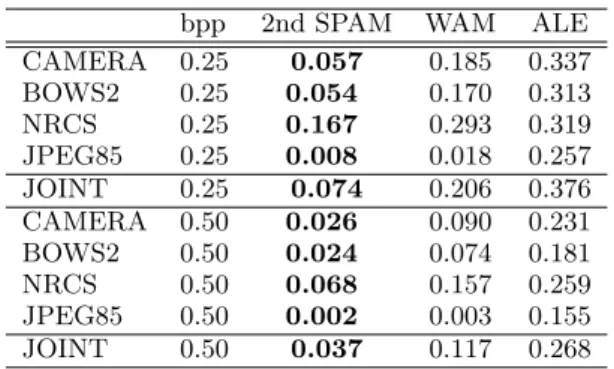
bpp 2nd SPAM WAM ALE CAMERA 0.25 0.057 0.185 0.337 BOWS2 0.25 0.054 0.170 0.313 NRCS 0.25 0.167 0.293 0.319 JPEG85 0.25 0.008 0.018 0.257 JOINT 0.25 0.074 0.206 0.376 CAMERA 0.50 0.026 0.090 0.231 BOWS2 0.50 0.024 0.074 0.181 NRCS 0.50 0.068 0.157 0.259 JPEG85 0.50 0.002 0.003 0.155 JOINT 0.50 0.037 0.117 0.268 Table 3: Error (2) of steganalyzers for LSB matching with payloads 0.25 and 0.5 bpp. The steganalyzers were implemented as SVMs with a Gaussian kernel. The lowest error for a given database and message length is in boldface.
a particular payload. The reported error (2) was always measured on images from the testing set, which were not used in any form during training or development of the ste-ganalyzer.
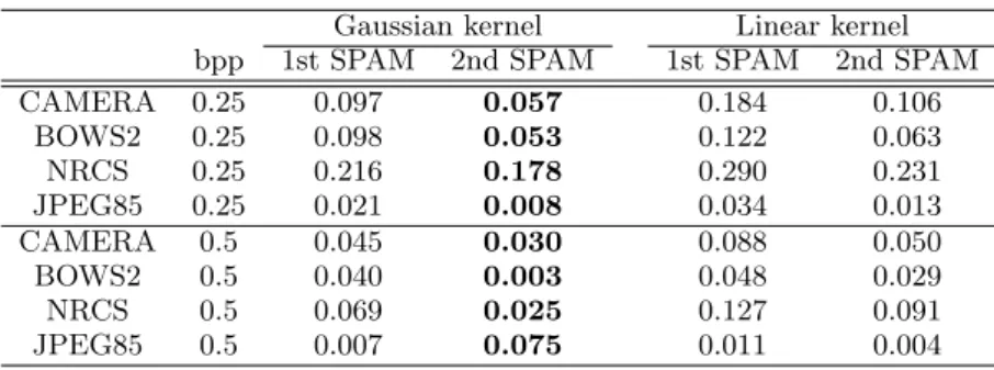
Results, summarized in Table 3.2, show that steganalyzers implemented as Gaussian SVMs are always better than their linear counterparts. This shows that the decision bound-aries between cover and stego features are nonlinear, which is especially true for databases with images of different size (Camera, JPEG85). Moreover, the steganalyzers built from the second-order SPAM model with differences in the range [−3, +3] are also always better than steganalyzers based on first-order SPAM model with differences in the range [−4, +4], which indicates that the degree of the model is more important than the range of the differences.
3.3 Comparison with prior art
Table 3 shows the classification error (2) of the steganalyz-ers using second-order SPAM (686 features), WAM [8] (81 features), and ALE [5] (10 features) on all four databases and for two relative payloads. We have created a special steganalyzer for each combination of the database, features, and payload (total 4×3×2 = 24 steganalyzers). The stegan-alyzers were implemented by SVMs with a Gaussian kernel as described in Section 3.1.2.
Table 3 also clearly demonstrates that the accuracy of steganalysis greatly depends on the cover source. For im-ages with a low level of noise, such as JPEG-compressed images, the steganalysis is very accurate (PErr = 0.8% on
images with payload 0.25 bpp). On the other hand, on very noisy images, such as scanned photographs from the NRCS database, the accuracy is obviously worse. Here, we have to be cautious with the interpretation of the results, because the NRCS database contains only 1500 images, which makes the estimates of accuracy less reliable than on other, larger image sets.
In all cases, the steganalyzers that used second-order SPAM features perform the best, the WAM steganalyzers are sec-ond with about three times higher error, and ALE stegan-alyzers are the worst. Figure 3 compares the steganstegan-alyzers in selected cases using the receiver operating characteristic curve (ROC), created by varying the threshold of SVMs with the Gaussian kernel. The dominant performance of SPAM steganalyzers is quite apparent.
4. CURSE OF DIMENSIONALITY
Denoting the number of training samples as l and the number of features as d, the curse of dimensionality refers to overfitting the training data because of an insufficient number of training samples and a large dimensionality d (e.g., the ratio l
d is too small). In theory, the number of
training samples depends exponentially on the dimension of the training set, but the practical rule of thumb states that the number of training samples should be at least ten times the dimension of the training set.
One of the reasons for the popularity of SVMs is that they are considered resistant to the curse of dimensionality and to uninformative features. However, this is true only for SVMs with a linear kernel. SVMs with the Gaussian kernel (and other local kernels as well) can suffer from the curse of dimensionality and their accuracy can be decreased by uninformative features [3]. Because the dimensionality of the second-order SPAM feature set is 686, the feature set may be susceptible to all the above problems, especially for experiments on the NRCS database.
This section investigates whether the large dimensionality and uninformative features negatively influence the perfor-mance of the steganalyzers based on second-order SPAM features. We use a simple feature selection algorithm to select subsets of features of different size, and observe the discrepancy between the errors on the training and testing sets. If the curse of dimensionality occurs, the difference between both errors should grow with the dimension of the feature set.
4.1 Details of the experiment
The aim of feature selection is to select a subset of fea-tures so that the classifier’s accuracy is better or equal to the classifier implemented using the full feature set. In the-ory, finding the optimal subset of features is an NP-complete problem [9], which frequently suffers from overfitting. In or-der to alleviate these issues, we used a very simple feature selection scheme operating in a linear space. First, we cal-culated the correlation coefficient between the ithfeature x
i
and the number of embedding changes in the stego image y according to6
corr(xi, y) = p E[xiy]− E[xi]E[y]
E[x2
i]− E[xi]2·
p
E[y2]− E[y]2 (3)
Second, a subset of features of cardinality k was formed by selecting k features with the highest correlation coefficient.7
The advantages of this approach to feature selection are a good estimation of the ranking criteria, since the features are evaluated separately, and a low computational complexity. The drawback is that the dependences between multiple fea-tures are not evaluated, which means that the selected sub-sets of features are almost certainly not optimal, i.e., there exists a different subset with the same or smaller number of features with a better classification accuracy. Despite this weakness, the proposed method seems to offer a good
6In Equation (3), E[
·] stands for the empirical mean over the variable within the brackets. For example E[xiy] =
1 n
Pn
j=1xi,jyj, where xi,j denotes the ith element of the jth
feature vector.
7This approach is essentially equal to feature selection
us-ing the Hilbert-Schmidt independence criteria with linear kernels [22].
Gaussian kernel Linear kernel bpp 1st SPAM 2nd SPAM 1st SPAM 2nd SPAM CAMERA 0.25 0.097 0.057 0.184 0.106 BOWS2 0.25 0.098 0.053 0.122 0.063 NRCS 0.25 0.216 0.178 0.290 0.231 JPEG85 0.25 0.021 0.008 0.034 0.013 CAMERA 0.5 0.045 0.030 0.088 0.050 BOWS2 0.5 0.040 0.003 0.048 0.029 NRCS 0.5 0.069 0.025 0.127 0.091 JPEG85 0.5 0.007 0.075 0.011 0.004
Table 2: Minimal average decision error (2) of steganalyzers implemented using SVMs with Gaussian and linear kernels on images from the testing set. The lowest error for a given database and message length is in boldface. 0 0.2 0.4 0.6 0.8 1 0 0.2 0.4 0.6 0.8 1
False positive rate
D et ec ti on ac cu rac y 2nd SPAM WAM ALE
(a) CAMERA, payload = 0.25bpp
0 0.2 0.4 0.6 0.8 1 0 0.2 0.4 0.6 0.8 1
False positive rate
D et ec ti on ac cu rac y 2nd SPAM WAM ALE (b) CAMERA, payload = 0.50bpp 0 0.2 0.4 0.6 0.8 1 0 0.2 0.4 0.6 0.8 1
False positive rate
D et ec ti on ac cu rac y 2nd SPAM WAM ALE (c) JOINT, payload = 0.25bpp 0 0.2 0.4 0.6 0.8 1 0 0.2 0.4 0.6 0.8 1
False positive rate
D et ec ti on ac cu rac y 2nd SPAM WAM ALE (d) JOINT, payload = 0.50bpp
Figure 3: ROC curves of steganalyzers using second-order SPAM, WAM, and ALE features calculated on CAMERA and JOINT databases.
trade-off between computational complexity, performance, and robustness.
We created feature subsets of dimension d∈ D, D = {10, 20, 30, . . . , 190, 200, 250, 300, . . . , 800, 850}. For each subset, we trained an SVM classifier with a Gaus-sian kernel as follows. The training parameters C, γ were selected by a grid-search with five-fold cross-validation on the training set as explained in Section 3.1.2. Then, the SVM classifier was trained on the whole training set and its accuracy was estimated on the testing set.
4.2 Experimental results
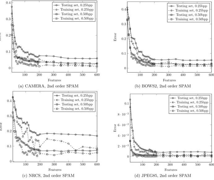
Figure 4 shows the errors on the training and testing sets on four different databases. We can see that even though the error on the training set is smaller than the error on the testing set, which is the expected behavior, the differences are fairly small and do not grow with the feature set dimen-sionality. This means that the curse of dimensionality did not occur.
The exceptional case is the experiment on the NRCS database, in particular the test on stego images with payload 0.25 bpp. Because the training set contained only ≈ 1400 examples (700 cover and 700 stego images), we actually expected the curse of dimensionality to occur and we included this case as a reference case. We can observe that the training error is rather erratic and the difference between training and test-ing errors increases with the dimension of the feature set. Surprisingly, the error on the testing set does not grow with the size of the feature set. This means that even though the size of the training is not sufficient, it is still better to use all features and rely on regularization of SVMs to prevent overtraining rather than to use a subset of features.
4.3 Discussion of feature selection
In agreement with the findings published in [18, 20], our results indicate that feature selection does not significantly improve steganalysis. The authors are not aware of a case when a steganalyzer built from a subset of features provided significantly better results than a classifier with a full feature set. This remains true even in extreme cases, such as our experiments on the NRCS database, where the number of training samples was fairly small.
From this point of view, it is a valid question whether feature selection provides any advantages to the stegana-lyst. The truth is that the knowledge of important features reveals weaknesses of steganographic algorithms, which can help design improved versions. At the same time, the knowl-edge of the most contributing features can drive the search for better feature sets. For example, for the SPAM features we might be interested if it is better to enlarge the scope of the Markov model by increasing its order or the range of differences, T . In this case, feature selection can give us a hint. Finally, feature selection can certainly be used to re-duce the dimensionality of the feature set and consequently speed up the training of classifiers on large training sets. In experiments showed in Figure 4, we can see that using more than 200 features does not bring a significant improvement in accuracy. At the same time, one must be aware that the feature selection is database-dependent as only 114 out of 200 best features were shared between all four databases.
5. CONCLUSION
The majority of steganographic methods can be inter-preted as adding independent realizations of stego noise to the cover digital-media object. This paper presents a novel approach to steganalysis of such embedding methods by uti-lizing the fact that the noise component of typical digital me-dia exhibits short-range dependences while the stego noise is an independent random component typically not found in digital media. The local dependences between differences of neighboring pixels are modeled as a Markov chain, whose sample probability transition matrix is taken as a feature vector for steganalysis.
The accuracy of the steganalyzer was evaluated and com-pared with prior art on four different image databases. The proposed method exhibits an order of magnitude lower av-erage detection error than prior art, consistently across all four cover sources.
Despite the fact that the SPAM feature set has a high dimension, by employing feature selection we demonstrated that curse of dimensionality did not occur in our experi-ments.
In our future work, we would like to use the SPAM fea-tures to detect other steganographic algorithms for spatial domain, namely LSB embedding, and to investigate the lim-its of steganography in the spatial domain to determine the maximal secure payload for current spatial-domain embed-ding methods. Another direction worth pursuing is to use the third-order Markov chain in combination with feature selection to further improve the accuracy of steganalysis. Finally, it would be interesting to see whether SPAM-like features can detect steganography in transform-domain for-mats, such as JPEG.
6. ACKNOWLEDGMENTS
Tom´aˇs Pevn´y and Patrick Bas are supported by the Na-tional French projects Nebbiano 06-SETIN-009, ANR-RIAM Estivale, and ANR-ARA TSAR. The work of Jessica Fridrich was supported by Air Force Office of Scientific Re-search under the reRe-search grant number FA9550-08-1-0084. The U.S. Government is authorized to reproduce and dis-tribute reprints for Governmental purposes notwithstanding any copyright notation there on. The views and conclusions contained herein are those of the authors and should not be interpreted as necessarily representing the official policies, either expressed or implied of AFOSR or the U.S. Govern-ment. We would also like to thank Mirek Goljan for provid-ing the code for extraction of WAM features, and Gwena¨el Do¨err for providing the code for extracting ALE features.
7. REFERENCES
[1] http://photogallery.nrcs.usda.gov/. [2] P. Bas and T. Furon. BOWS–2.
http://bows2.gipsa-lab.inpg.fr, July 2007.
[3] Y. Bengio, O. Delalleau, and N. Le Roux. The curse of dimensionality for local kernel machines. Technical Report TR 1258, Universit´e de Montr´eal, Dept. IRO, Universit´e de Montr´eal, P.O. Box 6128, Downtown Branch, Montreal, H3C 3J7, QC, Canada, 2005. [4] G. Cancelli, G. Do¨err, I. Cox, and M. Barni. A
comparative study of±1 steganalyzers. In Proceedings IEEE, International Workshop on Multimedia Signal
100 200 300 400 500 600 0 0.1 0.2 0.3 0.4 Features E rr or Testing set, 0.25bpp Training set, 0.25bpp Testing set, 0.50bpp Training set, 0.50bpp
(a) CAMERA, 2nd order SPAM
100 200 300 400 500 600 0 0.1 0.2 0.3 0.4 Features E rr or Testing set, 0.25bpp Training set, 0.25bpp Testing set, 0.50bpp Training set, 0.50bpp
(b) BOWS2, 2nd order SPAM
100 200 300 400 500 600 0 0.1 0.2 0.3 0.4 Features E rr or Testing set, 0.25bpp Training set, 0.25bpp Testing set, 0.50bpp Training set, 0.50bpp (c) NRCS, 2nd order SPAM 100 200 300 400 500 600 0 2 · 10−2 4 · 10−2 6 · 10−2 8 · 10−2 0.1 Features E rr or Testing set, 0.25bpp Training set, 0.25bpp Testing set, 0.50bpp Training set, 0.50bpp
(d) JPEG85, 2nd order SPAM
Figure 4: Discrepancy between errors on training and testing set plot with respect to number of features. Dashed line: errors on training set, solid line: errors on the testing set.
Processing, pages 791–794, Queensland, Australia, October 2008.
[5] G. Cancelli, G. Do¨err, I. Cox, and M. Barni. Detection of±1 steganography based on the amplitude of histogram local extrema. In Proceedings IEEE, International Conference on Image Processing, ICIP, San Diego, California, October 12–15, 2008.
[6] J. Fridrich. Feature-based steganalysis for JPEG images and its implications for future design of steganographic schemes. In J. Fridrich, editor, Information Hiding, 6th International Workshop, volume 3200 of Lecture Notes in Computer Science, pages 67–81, Toronto, Canada, May 23–25, 2004. Springer-Verlag, New York.
[7] J. Fridrich and M. Goljan. Digital image
steganography using stochastic modulation. In E. J. Delp and P. W. Wong, editors, Proc. SPIE, Electronic Imaging, Security, Steganography, and Watermarking of Multimedia Contents V, volume 5020, pages 191–202, Santa Clara, CA, January 21–24, 2003. [8] M. Goljan, J. Fridrich, and T. Holotyak. New blind
steganalysis and its implications. In E. J. Delp and P. W. Wong, editors, Proc. SPIE, Electronic Imaging, Security, Steganography, and Watermarking of Multimedia Contents VIII, volume 6072, pages 1–13, San Jose, CA, January 16–19, 2006.
[9] I. Guyon, S. Gunn, M. Nikravesh, and L. A. Zadeh. Feature Extraction, Foundations and Applications. Springer, 2006.
[10] J. J. Harmsen and W. A. Pearlman. Steganalysis of additive noise modelable information hiding. In E. J. Delp and P. W. Wong, editors, Proc. SPIE, Electronic Imaging, Security, Steganography, and Watermarking of Multimedia Contents V, volume 5020, pages 131–142, Santa Clara, CA, January 21–24, 2003. [11] T. S. Holotyak, J. Fridrich, and S. Voloshynovskiy.
Blind statistical steganalysis of additive steganography using wavelet higher order statistics. In J. Dittmann, S. Katzenbeisser, and A. Uhl, editors,
Communications and Multimedia Security, 9th IFIP TC-6 TC-11 International Conference, CMS 2005, Salzburg, Austria, September 19–21, 2005.
[12] C. Hsu, C. Chang, and C. Lin. A Practical Guide to± Support Vector Classification. Department of
Computer Science and Information Engineering, National Taiwan University, Taiwan.
[13] J. Huang and D. Mumford. Statistics of natural images and models. In Proceedngs of IEEE Conference on Computer Vision and Pattern Recognition,
volume 1, page 547, 1999.
[14] A. D. Ker. A general framework for structural analysis of LSB replacement. In M. Barni, J. Herrera,
S. Katzenbeisser, and F. P´erez-Gonz´alez, editors, Information Hiding, 7th International Workshop, volume 3727 of Lecture Notes in Computer Science, pages 296–311, Barcelona, Spain, June 6–8, 2005. Springer-Verlag, Berlin.
[15] A. D. Ker. Steganalysis of LSB matching in grayscale images. IEEE Signal Processing Letters,
12(6):441–444, June 2005.
[16] A. D. Ker. A fusion of maximal likelihood and structural steganalysis. In T. Furon, F. Cayre,
G. Do¨err, and P. Bas, editors, Information Hiding, 9th International Workshop, volume 4567 of Lecture Notes in Computer Science, pages 204–219, Saint Malo, France, June 11–13, 2007. Springer-Verlag, Berlin. [17] A. D. Ker and R. B¨ohme. Revisiting weighted
stego-image steganalysis. In E. J. Delp and P. W. Wong, editors, Proc. SPIE, Electronic Imaging, Security, Forensics, Steganography, and Watermarking of Multimedia Contents X, volume 6819, San Jose, CA, January 27–31, 2008.
[18] A. D. Ker and I. Lubenko. Feature reduction and payload location with WAM steganalysis. In E. J. Delp and P. W. Wong, editors, Proceedings SPIE, Electronic Imaging, Media Forensics and Security XI, volume 6072, pages 0A01–0A13, San Jose, CA, January 19–21, 2009.
[19] X. Li, T. Zeng, and B. Yang. Detecting LSB matching by applying calibration technique for difference image. In A. Ker, J. Dittmann, and J. Fridrich, editors, Proc. of the 10th ACM Multimedia & Security Workshop, pages 133–138, Oxford, UK, September 22–23, 2008. [20] Y. Miche, P. Bas, A. Lendasse, C. Jutten, and
O. Simula. Reliable steganalysis using a minimum set of samples and features. EURASIP Journal on Information Security, 2009. To appear, preprint available on http:
//www.hindawi.com/journals/is/contents.html. [21] M. K. Mihcak, I. Kozintsev, K. Ramchandran, and
P. Moulin. Low-complexity image denoising based on statistical modeling of wavelet coefficients. IEEE Signal Processing Letters, 6(12):300–303, December 1999.
[22] L. Song, A. J. Smola, A. Gretton, K. M. Borgwardt, and J. Bedo. Supervised feature selection via dependence estimation. In C. Sammut and
Z. Ghahramani, editors, International Conference on Machine Learning, pages 823–830, Corvallis, OR, June 20–24, 2007.
[23] D. Soukal, J. Fridrich, and M. Goljan. Maximum likelihood estimation of secret message length embedded using±k steganography in spatial domain. In E. J. Delp and P. W. Wong, editors, Proc. SPIE, Electronic Imaging, Security, Steganography, and Watermarking of Multimedia Contents VII, volume 5681, pages 595–606, San Jose, CA, January 16–20, 2005.
[24] K. Sullivan, U. Madhow, S. Chandrasekaran, and B.S. Manjunath. Steganalysis of spread spectrum data hiding exploiting cover memory. In E. J. Delp and P. W. Wong, editors, Proc. SPIE, Electronic Imaging, Security, Steganography, and Watermarking of Multimedia Contents VII, volume 5681, pages 38–46, San Jose, CA, January 16–20, 2005.
[25] V. N. Vapnik. The Nature of Statistical Learning Theory. Springer-Verlag, New York, 1995.
[26] D. Zo, Y. Q. Shi, W. Su, and G. Xuan. Steganalysis based on Markov model of thresholded
prediction-error image. In Proc. of IEEE International Conference on Multimedia and Expo, pages 1365–1368, Toronto, Canada, July 9-12, 2006.