Chip-Scale Quadrupole Mass Filters
for a Micro-Gas Analyzer
by Kerry Cheung
B.S., Applied and Engineering Physics Cornell University, 2003
S.M., Electrical Engineering and Computer Science Massachusetts Institute of Technology, 2005
Submitted to the Department of Electrical Engineering and Computer Science in partial fulfillment of the requirements for the degree of
Doctor of Philosophy in Electrical Engineering and Computer Science at the
MASSACHUSETTS INSTITUTE OF TECHNOLOGY June 2009
© 2009 Massachusetts Institute of Technology All rights reserved
Author__________________________________________________________________ Department of Electrical Engineering and Computer Science
May 22, 2009 Certified by______________________________________________________________
Akintunde I. Akinwande Professor of Electrical Engineering and Computer Science Thesis Supervisor Accepted by_____________________________________________________________
Chip-Scale Quadrupole Mass Filters
for a Micro-Gas Analyzer
by Kerry Cheung
Submitted to the Department of Electrical Engineering and Computer Science on May 22, 2009 in partial fulfillment of the requirements for the degree of
Doctor of Philosophy in Electrical Engineering and Computer Science
Abstract
Mass spectrometers are powerful analytical instruments that serve as the gold standard for chemical analysis. This tool has numerous applications ranging from national security, industrial processing, environmental monitoring, space exploration, and healthcare to name a few. These systems are typically large, heavy, power-hungry, and expensive, constraining its usage to a laboratory setting. In recent years, there has been a growing interest in utilizing mass spectrometers outside the lab.
Microelectromechanical systems (MEMS) technology holds the promise of making devices smaller, faster, better, and cheaper. The Micro-Gas Analyzer (MGA) project attempts to leverage MEMS capabilities to create a low-cost, high-performance, portable mass spectrometer. Batch-fabrication of various components for the MGA has been demonstrated to date, but the mass filter component still has room for exploration.
Chip-scale quadrupole mass filters achieved entirely through wafer-scale processing have been designed, fabricated, and characterized. The device integrates the quadrupole electrodes, ion optics, and housing into a single monolithic block, eliminating the electrode-to-housing misalignments inherent in other quadrupoles. To achieve this integration, unconventional square electrode geometry was utilized. This concept formed the basis of the micro-square electrode quadrupole mass filter (MuSE-QMF).
The MuSE-QMF demonstrated mass filtering with a maximum mass range of 650 amu and a minimum peak-width of 0.5 amu at mass 40, corresponding to a resolution of 80. More importantly, the design concept can be extended to complex architectures that were previously unachievable. Batch-fabricated quadrupoles in arrays, in tandem, or with integrated pre-filters can have significant impact on the future of portable mass spectrometry. Additionally, the MuSE-QMF makes a case for operation in the second stability region, and motivates new studies on quadrupole ion dynamics.
Acknowledgements
As an applied and engineering physics major with little to no real world experience, graduate school seemed like the next logical step. Frank Wise, my undergraduate advisor, gave me fair warning of what to expect but it was still quite the journey. These past six years have been filled with challenges, struggles, and emotional turmoil, but I was fortunate enough to have an equal amount of rewards and accomplishments. I’ve learned so much and grown personally and professionally within this time, and I owe it all to the people who have supported me throughout the experience.
First and foremost, I would like to thank my advisor, Tayo Akinwande, for giving me the opportunity to work under his guidance. His faith in me and my abilities is what got me through the lows of my doctoral work. He sometimes pushed me when it was needed but was always supportive. Additionally, his compassion and understanding throughout life’s many ups and downs is something I am extremely grateful for. Next, I would like to thank my other committee members, Marty Schmidt and Forest White. Marty supervised my masters but he has never stopped providing excellent advice and feedback since. He has been a source of knowledge and I’ve learned many lessons from him, especially the importance of simple fabrication. I am also very grateful to have Forest onboard who was always enthusiastic about my research and helped me gauge the relevance of my work in the greater community.
Outside of my committee, there have been others who have given me excellent advice and assistance with issues that I encountered throughout this thesis work. I want to thank Luis Velásquez-García for many fruitful discussions and his experience with fabrication techniques. My work would not have been possible without some of his insights. Randy Pedder is another who has been instrumental in my work, and I am extremely thankful for his advice and patience. He has been a tremendous asset towards getting me caught up to speed on the field of mass spectrometry and the experimental work involved. I would also like to thank Thomas Hogan and Steve Taylor who have contributed a substantial amount of their time and resources to conduct simulations on my behalf. Appreciation goes to Hanqing Li for helpful feedback on fabrication issues as well.
I want to thank Vicky Diadiuk and the Microsystems Technology Laboratories staff for their training and assistance which were vital for my success in the cleanroom. I want to acknowledge Dennis Ward, Bob Bicchieri, Eric Lim, and Donal Jamieson for maintaining the tools needed to complete my devices and for their understanding when I caused tools to go down. I also want to thank Kurt Broderick, Paul Tierney, Dave Terry, Pat Varley, Pat Burkhart, Acia Adams, Debb Hodges-Pabon, Sam Crooks, Carolyn Collins, Anne Wasserman, and others members of the MTL community for their smiles and friendship through the years. Additionally, I want to thank the fab users of past and present – Annie Wang, Kevin Ryu, Orit Shamir, Nan Yang, Vikas Sharma, Ole Nielsen, Kishori Desphande, Andrea Adamo, Ivan Nausieda, Darius Golda, Linhvu, and others
My friends who kept me sane outside the cleanroom have my eternal gratitude. I want to thank Dave Chao, Karen Wong, Amil Patel, Tyrone Hill, Ming Tang, and Brian Taff for all the interesting lunch/dinner conversations. Sean Liu, Lila Gollogoly, and Michelle Tiu have my deepest appreciation for all the support and good times at 150 Franklin. Much love goes to Elisa Rah, Dave Nguyen, Helen Hsi, Nancy Hong, Tim Lu, John King, Rich Moy, and their circle of friends for the many fun-filled weekends. Also, I want to acknowledge Lindsay Calderon for being there when I was feeling my worst, and the MIT Asian American Association for giving me a purpose outside academics.
Finally, I would like to thank my family for being supportive of everything I choose to do. I thank my parents for working so hard to give me every opportunity they could, and my brother and extended family for always having faith in me. I would also like to thank my cousin, Amy Fung, for making Boston more fun, my friends from back home for keeping me grounded, and Hannah Seong for her love and affection. Lastly, I want to remember those I have lost along the way – Antimony Gerhardt who will always inspire me, my maternal grandmother who I will miss dearly, and Henney who will always be loved and adored. I dedicate this thesis to them all.
Table of Contents
Acknowledgements ... 5 Table of Contents ... 7 List of Figures... 9 List of Tables ... 11 1 Introduction... 13 1.1 Motivation... 13 1.2 Mass Spectrometers ... 14 1.2.1 Overview... 14 1.2.2 Mass Filters... 15 1.3 Miniaturization... 17 1.3.1 Benefits ... 17 1.3.2 Scaled-Down Components... 181.4 Micro-Gas Analyzer Project ... 19
1.5 Thesis Organization ... 21
2 Quadrupole Mass Filters ... 23
2.1 Quadrupole Physics ... 23
2.2 Mass Filtering ... 26
2.3 Quadrupole Performance ... 28
2.4 Non-linear Resonances ... 30
2.5 Higher Stability Regions... 32
2.6 MEMS-based Quadrupoles... 34 2.7 Summary ... 37 3 Device Design... 39 3.1 Scaling Considerations... 39 3.1.1 Performance ... 39 3.1.2 Capacitance ... 42 3.1.3 Pressure... 45 3.2 Device Concept... 46 3.3 Optimization ... 47 3.3.1 Multipole Expansion... 48 3.3.2 Results... 49 3.4 Integrated Optics... 52 3.5 Positional Tolerance... 54 3.6 Summary ... 55 4 MuSE version 1.0... 57 4.1 Overview... 57 4.2 Device Fabrication... 58 4.3 Fabrication Issues... 64 4.3.1 Deep Etching... 65 4.3.2 Bonding... 67 4.4 Characterization ... 68
4.5 Discussion... 74
4.6 Summary ... 76
5 QMF Characterization System... 77
5.1 Overview... 77
5.2 Components ... 78
5.2.1 Vacuum Chamber and Flange Mount ... 79
5.2.2 Drive Circuit and Electronics... 84
5.2.3 Control Software and Data Acquisition... 87
5.3 System Operation and Calibration... 90
5.4 Issues and Improvements... 92
5.5 Summary ... 93
6 MuSE version 1.5... 95
6.1 Overview... 95
6.2 New Process Flow... 96
6.2.1 Improvements ... 101 6.2.2 Issues... 102 6.3 Characterization ... 104 6.3.1 Experimentation... 105 6.3.2 Results... 106 6.4 Discussion... 115 6.5 Summary ... 118
7 New Ion Dynamics ... 119
7.1 Overview... 119
7.2 Modified Stability Regions ... 119
7.2.1 Mapping Technique ... 120
7.2.2 First Stability Region ... 122
7.2.3 Second Stability Region... 124
7.3 Modified Performance ... 126
7.4 Summary ... 130
8 Conclusions and Future Work ... 131
8.1 Conclusions... 131
8.2 Future Work... 132
8.2.1 MuSE version 2.0 and beyond... 132
8.2.2 Electronics... 134 8.2.3 Improved Studies ... 135 8.2.4 Integration... 135 8.3 Contributions... 136 A Process Flows... 137 B Mask Layouts ... 145 C MATLAB Scripts... 159 D LabVIEW Programming... 161 E Technical Drawings ... 167
F Test System Operating Instructions... 176
List of Figures
Figure 1-1: Schematic of mass spectrometer operation... 15
Figure 1-2: Overview of the Micro-Gas Analyzer... 19
Figure 1-3: Popular types of mass filters [48] ... 20
Figure 2-1: Ideal quadrupole field with hyperbolic electrodes... 23
Figure 2-2: Mathieu stability diagram ... 25
Figure 2-3: Schematic of mass filtering... 26
Figure 2-4: Scan-line for constant peak-width operation [53]... 27
Figure 2-5: Non-linear resonances in the first stability region [69]... 31
Figure 2-6: Upper and lower corners of the second stability region [78]... 33
Figure 2-7: V-shaped groove MEMS QMF [23] ... 35
Figure 2-8: Integrated Einzel lens for V-shaped groove MEMS QMF [81]... 35
Figure 2-9: Monolithic MEMS QMF [27]... 36
Figure 2-10: Out-of-plane MEMS QMF [47]... 36
Figure 2-11: Other MEMS-based QMFs [25], [26]... 37
Figure 3-1: Design space for a chip-scale QMF ... 41
Figure 3-2: Model for capacitance calculation ... 43
Figure 3-3: Device model for parasitic capacitances... 44
Figure 3-4: Paschen curve... 45
Figure 3-5: Technical progression of electrode geometries... 47
Figure 3-6: Geometries used for optimization ... 48
Figure 3-7: Optimization results for electrode dimensions... 50
Figure 3-8: Optimization results including the housing ... 51
Figure 3-9: Einzel lens configuration of integrated optics... 53
Figure 3-10: Misalignment effects [91] ... 55
Figure 4-1: Schematic of the MuSE-QMF... 58
Figure 4-2: Cross-sectional schematic of the MuSE-QMF under operation ... 58
Figure 4-3: Device cross-sectional schematic... 59
Figure 4-4: Cap wafer process flow... 60
Figure 4-5: Electrode wafer process flow... 61
Figure 4-6: Aperture wafer process flow ... 62
Figure 4-7: Final processing steps ... 63
Figure 4-8: Completed MuSE-QMF with US quarter ... 64
Figure 4-9: Cross-sectional SEMs of device ... 64
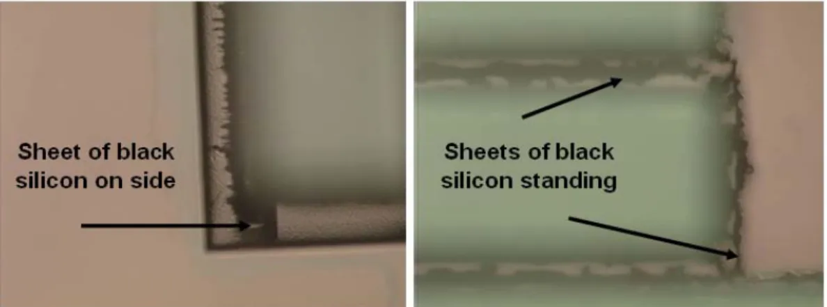
Figure 4-10: Remaining black silicon after electrode wafer DRIE ... 65
Figure 4-11: Etch non-idealities during recipe development... 66
Figure 4-12: Comparison between dies with good bonding and poor bonding... 67
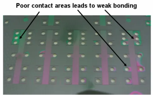
Figure 4-13: Dummy bond showing areas of poor contact... 68
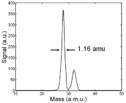
Figure 4-14: Mass spectrum of air at 3.8 MHz in the first stability region ... 70
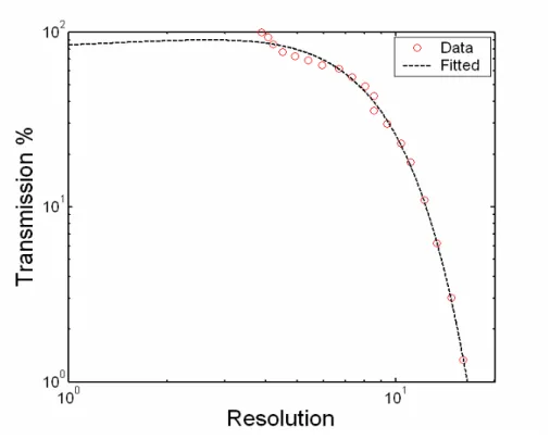
Figure 4-15: Resolution versus transmission curve using argon at 2.95 MHz ... 71
Figure 4-16: Mass spectrum of FC-43 at 1.98 MHz in the first stability region ... 72
Figure 5-2: Photographs of the in-house testing facility... 79
Figure 5-3: Flange mount schematic... 81
Figure 5-4: Assembled flange mount... 81
Figure 5-5: The peek testing jig... 82
Figure 5-6: Assembly of flange mount ... 83
Figure 5-7: Schematic of drive electronics ... 85
Figure 5-8: Drive circuit ... 85
Figure 5-9: Spice model of drive circuit ... 86
Figure 5-10: Screenshot of testing software ... 88
Figure 5-11: System calibration with macroscale quadrupole... 90
Figure 6-1: Differences between the two MuSE versions ... 95
Figure 6-2: New process flow for cap wafer ... 97
Figure 6-3: New process flow for aperture wafer... 98
Figure 6-4: New process flow for electrode wafer ... 99
Figure 6-5: Final processing of version 1.5 ... 100
Figure 6-6: Improvement in bond quality with new process flow... 102
Figure 6-7: Stringer formation on cap-electrode stack ... 103
Figure 6-8: SEMs showing shorting from stringers... 103
Figure 6-9: Electrode damage after ultrasonic cleaning ... 104
Figure 6-10: Detailed schematic of ionizer and device ... 106
Figure 6-11: Lens data at 3.5 MHz in the first stability region, 3.0 eV... 107
Figure 6-12: Lens data at 2.0 MHz in the second stability region, 5.0 eV ... 107
Figure 6-13: Pole bias data at 2.0 MHz in the first stability region, 3.0 eV ... 108
Figure 6-14: Mass spectra for air at various operating conditions... 109
Figure 6-15: Resolution versus transmission curves at various conditions ... 111
Figure 6-16: Mass spectrum of FC-43 at 1.8 MHz in the first stability region, 3.5 eV. 112 Figure 6-17: NIST library spectrum for FC-43... 112
Figure 6-18: Argon mass spectrum at 4.0 MHz in the first stability region, 3.0 eV ... 114
Figure 6-19: Argon mass spectrum at 2.0 MHz in the second stability region, 5.0 eV. 114 Figure 7-1: Typical scan-line ... 120
Figure 7-2: High resolution mapping... 121
Figure 7-3: Low resolution mapping ... 122
Figure 7-4: First stability region, 2.0 MHz ... 123
Figure 7-5: First stability region, 4.0 MHz ... 124
Figure 7-6: Second stability region, 2.0 MHz... 125
Figure 7-7: Best fit Mathieu stability diagram... 125
Figure 7-8: Resolution versus transmission curve at 1.5 MHz... 126
Figure 7-9: Performance comparisons of MEMS-based QMFs [23], [27], [47] ... 129
Figure 8-1: Electrode mask for MuSE version 2.0 ... 133
List of Tables
Table 3-1: Coefficients for different geometries and methods [91] ... 52
Table 3-2: Summary of device design ... 56
Table 4-1: Comparison between JBETCH and the etch recipe developed... 66
Table 5-1: 10-pin connection scheme ... 82
Table 5-2: Summary of filament supply ... 87
Chapter
1
Introduction
1.1 Motivation
As technology advances, there has been an increasing desire to know what is occurring in our surroundings. The ability to extract information from our environment is a great asset in making our machines, tools, and appliances smarter and better. From temperature sensors that regulate the heating and cooling of our homes and vehicles, to accelerometers and gyroscopes used in navigation, personal safety, and entertainment, sensors have become a part of our everyday lives.
If we draw a comparison to the five human senses, we have achieved the ability to “touch” (physical sensors), “see” (optical sensors), and “hear” (acoustic sensors). These sensors are able to provide us with sensitivities that surpass what is humanly possible. The capability to “taste” and “smell” lie within the domain of chemical sensors, which has limited developments to date. Chemical sensing of a few known species such as carbon monoxide, alcohol, or carbon dioxide can be readily accomplished, but the detectors are usually very specific and limited in speed, sensitivity, and lifetime.
Selective detectors operate through a reaction activated by absorption onto another compound or structure. These sensors are not very reliable since they are susceptible to contamination, saturation, and can be fooled by altering the specificity of a potentially hazardous compound. We would like to go beyond the limitations of selective detection, and provide fast, reliable chemical sensing for a wide range of substances. Developing
chemical and biological warfare agents, or possibly at airports and public spaces to monitor for explosives and other forms of terrorist threats. These sensors will also be extremely useful in the environment for the detection and regulation of pollutants or toxins that are introduced into our land, air, and water. Overall, the ability to detect and analyze known and unknown compounds is extremely beneficial, ensuring that many more applications will be discovered.
1.2 Mass Spectrometers
Mass spectrometers are powerful analytical instruments that serve as the gold standard for chemical analysis. The first mass spectrometer was reported in 1910 and was followed by 40 years of sporadic, but modest innovations [1]. Before the 1950’s, mass spectrometers only had a few applications in physics but this was soon changed with the growth of the petroleum industry. Commercialization of the mass spectrometer for chemical analysis pushed the rapid development of this tool. In turn, emphasis shifted from the physics of the device to finding new applications. Today, mass spectrometers are utilized in industrial processing, environmental monitoring, national security, space exploration, and healthcare to name a few.
1.2.1 Overview
A typical mass spectrometer is comprised of four main components – the ionizer, the mass filter, the detector, and the pump. The ionizer takes the gas sample to be analyzed, and turns them into ions by putting a charge on them. This enables the molecules to be directed and manipulated since they are neutral by nature. The ions then enter the mass filter, the core of the system, where they are sorted depending on their mass to charge ratios (m/e). Conditions are set so that only ions with a specific m/e are allowed to pass onto the detector where they are collected and counted. If we plot the detector count as a function of the specified m/e, we will generate a mass spectrum for the analyte. This spectrum will provide information on the relative quantities of each m/e within the sample, and serves as a chemical “finger print”. The last major component is the pump which keeps the other three components under vacuum. It is vital to have the gas mean
free path larger than the largest dimension of the mass spectrometer in order to prevent ions colliding with neutrals. Collisions will lead to discharging or the formation of complexes which negatively affect the analysis. Usually there are ion optics utilized between the ionizer, mass filter, and detector. These electrostatic lenses help couple ions into the mass filter and the filtered ions out to the detector. A schematic of typical mass spectrometer operation is shown in Figure 1-1.
Figure 1-1: Schematic of mass spectrometer operation
1.2.2 Mass Filters
Of the four major components that constitute a mass spectrometer, the one that determines the capabilities of the device is the mass filter. There are several methods to perform mass filtering, each with their advantages and disadvantages. Depending on the application, one method might be better suited than the others. Several of the more popular types of mass filters are the cross-field, the quadrupole, the ion trap, the time-of-flight, and the Fourier-transform ion cyclotron resonance [2].
The cross-field type relies on the Lorentz force exerted on a moving charge by an external magnetic field to perform the filtering. This mass filter is capable of very high resolution but is usually very large and heavy due to the magnets required. Additional disadvantages of this device are the associated cost, the non-linearity of the filtering mechanism, and the susceptibility of the performance to changes in pressure or the inlet
The quadrupole mass filter utilizes four parallel electrodes that are driven with a combination of d.c. and a.c. voltages to control the ion trajectories. Mass filtering is accomplished by scanning the voltages to produce stable and unstable trajectories for a given m/e. The main advantages of this type of mass filter are the device simplicity, the light weight, and the relative tolerance that the performance has to changes in pressure or ion energies. Additionally, mass scanning is linear and the sensitivity is high, but the key disadvantage is the limited resolution.
The ion trap is comprised of a ring electrode with ends caps and operates on the same principles as the quadrupole, namely the utilization of d.c. and a.c. voltages to control ion trajectories. The main advantages of this device are the compact size, and the ability to store the ions to be analyzed. Mass filtering is achieved by varying the voltage on an end cap to eject the desired m/e towards the detector. This mass filter is useful when the ion samples are limited, but there are potential issues with space-charge effects, storage efficiency, and limitations in resolution.
The time-of-flight mass filter operates on the principle of varying velocities for ions with different masses and the same kinetic energy. A burst of ions is released at the inlet, accelerated to the same potential, and allowed to separate in a long tube. Larger masses will fly slower, resulting in a later arrival time at the detector. The advantages of this device are the simplicity, the high sensitivity, the speed, and the ability to analyze very large masses. The disadvantages are the susceptibility to changes in the inlet condition, the need for very fast electronics to resolve light masses, and the non-linearity of the filtering mechanism.
The Fourier-transform ion cyclotron resonance type is quite complex and uses an interesting method for analysis. Ions are trapped within a cubic cell, and exposed to a magnetic field. Cyclotron motion is induced with an external pulse, and the resulting signal is detected and amplified. Performing a Fourier-transform on the amplified signal will produce a spectrum where the frequency is inversely related to m/e and the intensity is proportional to the number of ions with the same m/e. The key advantages of this device are the very high resolution, the ability to measure all the ions at once in a non-destructive manner, and the fact that there is an ion trap to hold limited samples. The
main disadvantages are the size, the cost, and potential issues with space-charge effects and storage efficiencies.
1.3 Miniaturization
If we are able to miniaturize a mass spectrometer and make it cheap enough, we will have the chemical sensor that we desire. With the growing demand for chemical analysis outside the laboratory, other researchers have identified the potential for scaled-down mass spectrometers. Substantial progress on the miniaturization of ion sources, mass filters, and detectors have been made but advances in small-scale pumps and valves are still limited. There is the option of implementing passive getter pumps, but this is not practical for long term usage. Other than the scaled-down components, appropriate drive electronics are needed before a fully miniaturized system can be realized. Ultimately, the performance may not match laboratory versions but there are applications where portable low-resolution devices are useful.
1.3.1 Benefits
Mass spectrometers are generally large, heavy, expensive, and power hungry due to the pumping requirements needed for proper operation. The main advantage of scaling-down is the relaxation on operational pressure [3]. Reduced dimensions will allow for higher pressures, enabling smaller, lighter, and cheaper vacuum pumps to be used. Once bulky, expensive pumps are removed from the system, portability becomes a viable option. Other benefits are the general reduction in size and weight of the mass filter component itself, the reductions in overall costs, and the increase in sensitivity associated with operation at higher pressures.
Portable mass spectrometers will have major contributions towards environmental monitoring, national security, and space exploration [4]. Field applications of mass spectrometers typically require samples to be obtained on-site and then taken back to a lab for analysis. This is highly inefficient, leading to delays and potential errors. In the case of national security, monitoring of explosives and other threats are limited to
are directly related to payloads so launching a conventional mass spectrometer into space will be very expensive. Development of a miniaturized mass spectrometer will address all these issues.
1.3.2 Scaled-Down Components
One direction for miniaturization is taking conventional machining technologies and using them to manufacture scaled-down components. Significant progress has been made by several groups on various types of mass filters using this method. Smith and Cromey reported making a small, inexpensive quadrupole from machined ceramics and stainless steel rods [5]. Ferran and Boumsellek demonstrated a quadrupole array formed from precision electrodes mounted into a glass base [6], [7]. Orient et al. also produced a quadrupole array but utilized precisions stainless steel electrodes and machineable ceramics [8]. Quadrupoles with hyperbolic electrodes have been reported by Holkeboer [9] and Wang [10]. Holkeboer et al. utilized electrical discharge machining to create the electrodes while Wang et al. machined a ceramic tube and coated the hyperbolic surfaces with a thin metal. Thorleaf Research Inc. (Santa Barbara, CA) demonstrated a miniature Paul ion trap used in conjunction with gas chromatography [11], while Oak Ridge National Laboratory (Oak Ridge, TN) reported a simple cylindrical ion trap [12]. Diaz et al. created an impressive double-focusing sector-field mass spectrometer [13], and Cooks’ group at Purdue University reported remarkable progress with a rectilinear ion trap [14], [15].
Another popular method for the miniaturization of mass spectrometers is the use of microfabrication technologies associated with microelectromechanical systems (MEMS) [16]. Microfabrication techniques allows for complex structures to be formed on a small scale with high precision. Most of the literature focuses on microfabricated mass filters and other individual components, but there are several reports that demonstrated fully integrated systems. For the mass filter, researchers have demonstrated cylindrical ion traps [17]-[19], a Wien filter [20], time-of-flight [21], and quadrupoles [22]-[27]. Novel concepts using traveling waves [28], and planar electrodes to form a Paul trap potential [29] have also been reported. Other microfabricated components such as hot filament ion sources [30], [31], electrospray ionizers [32], and micro-leak valves [33] have been
demonstrated successfully. Impressive work from Müller’s group from the Hamburg University of Technology (Hamburg, Germany) demonstrated an integrated system with a plasma ionizer, a time-of-flight mass filter, an energy filter, as well as a detector [34], [35]. A modification using a traveling wave mass filter has also been demonstrated [36]. Recently, the NASA Goddard Space Flight Center (Greenbelt, MD) reported a time-of-flight mass spectrometer assembled from various microfabricated components [37], [38].
1.4 Micro-Gas Analyzer Project
MEMS technology has become a reliable method for constructing complex geometries, and serves as a key enabler for the development of many small, low-cost, high-performance sensors [39]. The Micro-Gas Analyzer (MGA) project attempts to leverage the benefits of MEMS technology to develop a miniature mass spectrometer for portable chemical sensing. The system concept is shown in Figure 1-2 along with several images of microfabricated components that have been achieved to date by collaborators on the project.
For the ionizer, Chen et al. developed double-gated carbon nano-tube (CNT) field ionizer arrays capable of generating ions at very low powers [40], [41]. An open architecture CNT ionizer has also been fabricated by Velásquez-García [42], [43], where the design facilitates gas transport to the ionizer tips. For the detector, Zhu et al. reported an electrometer made from SOI technology that demonstrated an extremely low noise floor [44], [45]. Additionally, a silicon resonant beam mass detector can be fabricated alongside the electrometer for parallel detection [46]. Unpublished work by Vikas Sharma at the Massachusetts Institute of Technology demonstrated a micro-displacement vacuum pump that was able to pull down 220 Torr from atmosphere.
Out-of-plane quadrupole mass filters assembled using silicon deflection springs in a MEMS platform has been demonstrated as well [47]. Quadrupoles were implemented because of their simplicity, and robustness under operation. Figure 1-3 shows three popular types of mass filters that were considered for microfabrication due to their simple construction. From the fundamental equation of operation provided under each type of device, we can clearly see that the quadrupole is the best suited for scaling-down.
Figure 1-3: Popular types of mass filters [48]
If we make the magnetic sector device smaller (decrease r), an increase in the magnetic field B will be needed to maintain operation (m/e unchanged). This will require
larger and heavier magnets which is undesirable for miniaturization. If we scale-down the time-of-flight device (decrease L), then the ion flight times, τ, will also decrease to maintain operation. As a result, very fast electronics will be needed to detect light ions which might not be achievable. For the quadrupole field device, as the mass filter scales-down (smaller r0), the drive voltage V reduces quite substantially. An additional benefit
of this device is that the equation of operation has no dependence on the ion energy Vion.
Ion energy can be difficult to maintain accurately and will significantly impact the performance of the other types of mass filters.
For the MGA to become a ubiquitous gas sensor, the total system must be affordable. The low costs associated with MEMS sensors are achieved through batch-fabrication and economy of scale. Currently, the only component of the MGA that is not entirely batch-fabricated is the mass filter. The post-fabrication electrode assembly needed for the out-of-plane quadrupoles will serve as a bottleneck to mass production. This issue should be addressed, forming the basis of this thesis.
1.5 Thesis Organization
In this chapter, we identified several applications that are in need of fast, reliable chemical sensors. Mass spectrometers have the potential to fulfill this need if they can be miniaturized. The Micro-Gas Analyzer project aims to leverage MEMS technology to develop a low-cost, high-performance chemical sensor. Current limitations with the mass filter component prompts further exploration. The goal of this thesis was to address these limitations through the development of a chip-scale quadrupole mass filter.
The rest of this thesis is organized as follows – Chapter 2 introduces the theory behind quadrupole mass filter operation, and provides definitions for several relevant performance metrics. A summary of prior work on MEMS-based quadrupole mass filters is also included to put this thesis into perspective. Chapter 3 outlines the scaling considerations, and the optimization process used to arrive at the final device design. Chapter 4 covers the fabrication steps and experimental characterization for the first generation of chip-scale quadrupole mass filters. Chapter 5 details the design,
device characterization. Chapter 6 covers the improvements made to our initial device design, and outlines a modified fabrication process flow. Extensive characterization of the improved devices using the in-house testing facility is also reported. Chapter 7 investigates several interesting phenomena encountered during the testing of our new devices, while Chapter 8 summarizes the work in this thesis and makes recommendations for future directions.
Chapter
2
Quadrupole Mass Filters
2.1 Quadrupole Physics
To fully appreciate the power and simplicity of a quadrupole mass filter (QMF), a review of the underlying physics of operation is provided. As the name implies, the fundamental principle behind this type of mass filter is the quadrupole field. When four hyperbolic electrodes are placed symmetrically in space with the electric potentials shown in Figure 2-1, an ideal quadrupole field is established. This field can be expressed in Cartesian coordinates as 2 0 2 2 0 2 ) ( ) , ( r y x y x = Φ − Φ (2-1)
where r0 is the radius of the circle that is tangent to all four electrodes, and Ф0 is the
If the applied potential to each electrode is a combination of d.c. and a.c. voltages, |Ф0/2| = U – V cos (ωt), the equations of motion for an ion in the field will be
[
cos( )]
0 2 2 0 2 2 = − + U V t x mr e dt x d ω (2-2)[
cos( )]
0 2 2 0 2 2 = − − U V t y mr e dt y d ω (2-3)where e and m are the charge and the mass of the ion, U is the amplitude of the d.c. drive component, and V and ω are the amplitude and frequency of the a.c. component respectively. Typically, ω is in the range of radio frequencies (r.f.) for most practical applications so “a.c.” will be referred to as “r.f.” throughout this thesis.
From Equations 2-2 and 2-3, we see that ion motion in the x and y directions are independent of one another, decoupling the problem and allowing it to be solved more readily. By making the substitutions ux = x/r0, uy = y/r0, and ξ = ωt/2, we obtain the
Mathieu-like equations 0 ))] ( 2 cos( 2 [ 0 , 2 , 2 = − − ± xy y x a q u d u d ξ ξ ξ (2-4) 2 0 2 8 r m eU a ω = (2-5) 2 0 2 4 r m eV q ω = (2-6)
where a and q are known as the Mathieu parameters, and ξ0 corresponds to the initial r.f.
phase in which the ion enters the field. Equation 2-4 has a general solution in the form
∑
∑
∞ −∞ = − − ∞ −∞ = + = n in n n in ne e C e C e u α µξ ξ α µξ 2 ξ 2 2 2 " ' (2-7)where α’ and α” are constants that depend on the initial conditions, and the constants C2n
and µ depend only on the Mathieu parameters [1]. This fundamental property of the Mathieu equation means the nature of ion motion in the quadrupole will depend only on a and q, and not on the initial conditions.
Looking at Equation 2-7, we see that if µ is complex or real and non-zero, the solutions will be unstable due to the eµξ and e-µξ terms. When µ = iβ and is purely imaginary, the solutions will be periodic and stable for non-integer values of β, and will be periodic but unstable for integer values [1]. The periodic and stable solutions are the ones that are useful in a QMF, highlighting the true power of this type of mass filter. The filtering property is defined only by trajectory stabilities that are governed by the Mathieu parameters, independent of initial conditions. Filtering will only be affected by initial conditions in the sense that trajectories with amplitudes greater or equal to the confines of the device (r0) will not be transmitted.
The stable and unstable solutions of the Mathieu equation can be mapped as a function of the Mathieu parameters. The boundaries defining the regions shown in Figure 2-2 correspond to the integer values for β. From Equation 2-4, we see that the stability diagram will be symmetric about the a-axis, and that the boundaries stemming from positive a values correspond to the motion in the x-axis. Boundaries stemming from negative a values correspond to motion in the y-axis, so regions in which both stability diagrams overlap denote values of a and q in which ion motion is stable in both x and y. These sets of a and q form stability regions that are shaded and labeled in Figure 2-2. If the quadrupole is operated at an (a, q) near the corner of a stability region, mass filtering is achieved.
2.2 Mass Filtering
Given an operating frequency and characteristic device dimension (r0), we can use
Equation 2-5, 2-6, and the Mathieu stability diagram to calculate the range of U and V that will produce stable trajectories for a specific m/e. If the quadrupole is operated at a point near the corner of a stability region, there will be a small range of U and V that will transmit the specified ions. This range of voltages will be proportional to the peak-width of the detected signal, so a higher resolution mass peak is associated with a smaller range. A mass spectrum can be generated if the d.c. and r.f. voltages are scanned in a fixed ratio a/q = 2U/V, and the number of transmitted ions for each m/e is recorded. Figure 2-3 depicts the mass filtering principle for operation in the first stability region. Assuming an ion with m/z = 219 and the scan-line shown, the points along the scan-line that are within the stability region (green) will produce stable trajectories that transmit through the quadrupole and into the detector. Points that lie outside the stability region (red) will produce unstable trajectories that collide into the electrodes and discharge. The quantity m/z is often used interchangeably with m/e, where z corresponds to the number of charges on an ion of mass m.
Most commercial quadrupoles utilize cylindrical electrodes instead of hyperbolic ones due to the manufacturing simplicity. Researchers have found that cylindrical electrodes with radius r serve as a good approximation to ideal hyperbolic electrodes if the r-to-r0 ratio is 1.148 [49]. This number corresponds to the ratio needed to eliminate
the dodecapole term associated with using cylindrical electrodes, and was later revised to 1.145 [50]. Recent work using advanced simulations involving actual ion flight report an optimal value of 1.128 [51], [52]. Despite these approximations, there are still non-idealities that degrade performance and will be addressed in Section 2.3.
From Figure 2-3, we see that the peak-width of the detected signal becomes wider at larger masses. This is a direct result of the linear scan-line used, and is often referred to as the constant resolution mode since every peak has the same resolution. Commercial systems typically utilize a constant peak-width mode where the peak-width stays the same for every peak. This mode is more useful since it ensures proper mass separation throughout the range of the scanned masses. In turn, the resolution will be increasing for larger and larger masses, and the detected signals will decrease. The relative abundance of the analyte may be skewed, but proper calibration and tuning can address this issue. Ideally, mass spectra with constant peak-widths are produced by using a non-linear scan-line (dashed scan-line) as depicted in Figure 2-4. An approximation to this curved scan-scan-line can be achieved by assuming a linear scan-line with a non-zero intercept called ∆m, and a slope called ∆res [53]. For each system, these values are determined empirically through calibration with a low-mass ion and a high-mass ion simultaneously.
2.3 Quadrupole Performance
The performance of a QMF can be characterized by two key metrics, the mass range and the resolution. The mass range is the maximum mass resolvable with a quadrupole of radius r0 given a set of operating conditions. The operating point (a, q), the drive
frequency, and the maximum applied voltage will affect this metric, but it is ultimately constrained by the electrical breakdown of the QMF and the voltages that can be supplied by the drive electronics. The resolution is the more important performance metric, and is an indicator of how well the quadrupole can distinguish between ions with m/e that are close in value. Resolution is expressed as the ratio R = m/∆m, where m is the mass corresponding to the peak detected and ∆m is the peak full-width at half the maximum signal intensity (FWHM). Other researchers use different definitions for the peak-width (10% or 25% signal intensity) but this thesis will use the FWHM definition. The closer the quadrupole is operated to the corner of a stability region, the smaller the peak-width and the higher the resolution. Theoretically, the resolution can be infinite but in a real device with finite length, the maximum resolution attainable is limited by n, the number of r.f. cycles that an ion spends in the QMF [1].
Since the filtering mechanism of the quadrupole is based on ion trajectories with an oscillatory nature dictated by the drive frequency, we would expect the resolution to have a dependence on the value of n. Experimental data has shown that the resolution can be related to n by p n h m m R ≈ 1 ∆ = (2-8)
where h is a constant that reflects the operating point (a, q) as well as how the ionizer is coupled to the quadrupole, and p has been empirically determined to be about 2. A good approximation for n can be given by fL/vz where f is the drive frequency, L is the
quadrupole length, and vz is the axial ion velocity. If the ion is accelerated with a
potential Vz, then the resolution can be expressed as
= ≈ ≅ e V m L f h v L f h h n R z z 2 1 1 2 2 2 2 (2-9)
Combining Equation 2-8 and 2-9 and solving for ∆m, we get 2 2 2 L f e V h m= z ∆ (2-10)
which means the peak-width achievable is independent of mass. This result supports the constant peak-width mode of operation, but Equation 2-10 does not factor in field imperfections that limit the maximum resolution attainable.
Field imperfections can arise from either (1) misalignment of the electrodes, (2) the use of non-hyperbolic electrodes, (3) imbalances in the drive signals, or (4) static charges resulting from electrode contamination [1], [54]. The impact of each of these reasons on the resolution is not very well understood, but there have been reports which estimate the maximum resolving power as a function of misalignments [1], [54]. Since the filtering mechanism of a quadrupole (stable ion trajectories) depends on the established electric fields, distortions arising from construction errors such as electrode misalignments or variations in electrode diameters will degrade performance. A first-order approximation for the maximum resolution attainable from a QMF with construction error ε can be given by Rmax ~ 2r0/ε, where r0 is the characteristic dimension of the device. The other
reasons listed for field imperfections have been reported to have a direct impact on peak-shape. The formation of a precursor peak in the low-mass tails of the mass spectrum has been attributed to the use of circular electrodes [55], [56], while imbalances in the drive signals and contamination issues have been reported to cause peak-splitting [54], [57]. These undesirable features stem from non-linear resonances that will be discussed more extensively in Section 2.4.
Other performance metrics for a quadrupole are the abundance sensitivity and the transmission, but these quantities are not well understood. The abundance sensitivity is a measure of how “clean” a peak is, namely how much signal from mass M overlaps onto masses M-1 or M+1. Typically, this value is calculated by taking the ratio of the signal at mass M and the signal at M-0.5 or M+0.5. Larger values correspond to better abundance sensitivities since adjacent peaks will be more distinct. Ion energies, field imperfections, and fringing-fields arising from the finite length of the quadrupole electrodes will all impact this quantity in different ways that is not very predictable [56], [58]-[61]. These
abundance sensitivity. The transmission is measured as the percentage of incoming ions that make it through the device after filtering. This quantity is proportional to the quadrupole acceptance which is an electronically controlled aperture that depends on the ion dynamics. For a given operating condition, the acceptance signifies the area of the quadrupole inlet which allows ions to pass for all initial r.f. phases [62]. It is important to keep in mind that there are points that lie outside the quadrupole acceptance which can transmit ions for certain phases but not all. To further confuse things, the acceptance is affected by fringing-fields, the drive frequency, and the operating point (a, q) [60], [62], [63]. General trends are that fringing-fields and increased drive frequencies will decrease acceptance, and operation at higher resolution will decrease transmission.
Aside from the factors mentioned above, the ionizer, detector, ion lenses, and drive electronics also impact the performance of a quadrupole. For the ionizer, the ion energy used and the ionizer emittance will affect the transmission, abundance sensitivity, as well as peak-shapes. Large ion energies usually improve transmission but degrade abundance sensitivity and peak-shape since ions spend less time being filtered [59]. Typically, ion lenses are utilized to match the ionizer emittance to the quadrupole acceptance in order to improve overall performance. The same concept can be applied to the detector end of the device to couple filtered ions into the detector. Drive electronic stability is another key factor that impacts resolution [54]. Since the operating point (a, q) is set by the drive voltages, fluctuations in the 2U/V ratio during scanning can cause severe limitations in the maximum resolution attainable. Care should be taken during the drive circuit design to ensure signal precision and invariance to heating or drifts.
2.4 Non-linear Resonances
In an ideal QMF, the equations of motion for the x-axis and y-axis are independent from one another. Field imperfections arising from the factors mentioned in Section 2.3 will couple the equations of motion, changing the solutions of the Mathieu equation. The coupling will manifest as non-linear resonances that degrade peak-shape by introducing precursor peaks and peak-splitting. Substantial research has been conducted with Paul traps that demonstrated non-linear resonances with a good match to theory [64]-[67].
Linear Paul traps were later investigated and displayed the existence of non-linear resonances as well [68], [69]. These resonances effectively introduce lines of instability within the stability diagram as depicted in Figure 2-5. These new lines correspond to values of a and q that produce unstable ion trajectories that normally should be stable without the presence of the field imperfections.
Figure 2-5: Non-linear resonances in the first stability region [69]
The location of the instability lines shown in Figure 2-5 follows the theory that has been laid out by Wang et al. [70]. The resonance conditions of the coupled ion motion in a linear quadrupole are given by
ν β β = + y y x x n n 2 2 (2-11) N n nx + y = (2-12)
where nx, ny, ν, N are integers, and βx, βy are the characteristic exponents of the Mathieu
equation that depends on a and q. The integer N corresponds to the order of the non-ideal field components arising from field imperfections, and are only considered for values
If we imagine a scan-line that passes through the modified stability region shown in Figure 2-5, it is clear that several of these non-linear resonance lines will be crossed. As a result, the mass spectrum will have noding and peak-splitting that correspond to the unstable ion trajectories along the scan. Interestingly, the peak-splitting associated with these non-linear resonances are not as pronounced for low-resolution scans [71]. This result is due to the fact that the transmission is high and abundance sensitivity is small at low resolutions. The effects of the non-linear resonances are essentially smeared and hidden within the spectrum. Conversely, the peak-splitting and noding will be much more dramatic at high resolutions leading to a substantial degradation in peak-shape.
2.5 Higher Stability Regions
In Section 2.2, we introduced the Mathieu stability diagram which maps the stable and unstable solutions of the Mathieu equation. The boundaries shown in Figure 2-2 correspond to integer values of β, and provide information on the oscillatory nature of the ion trajectories in the quadrupole. Stable trajectories with a larger value of β will have a higher fundamental frequency of ion motion. From Figure 2-2, we can identify the three stability regions where ion motion will be stable in both x and y. Theoretically, there are a large number of these stability regions but only operation in the labeled three makes sense. The others regions are located at much larger a and q values which translates to significantly higher voltages that are not practical to implement. Operation in the first stability region correspond to 0 < β < 1, while operation in the third stability region correspond to 1 < β < 2. The second stability region is essentially a combination of the first and third stability regions with 0 < β < 1 and 1 < β < 2, and if often referred to as the intermediate stability region.
Most studies on quadrupole mass filters are conducted in the first stability region, but there have been reports of improved performance with operation in the second stability region [72]-[75]. Resolution is improved due to the higher fundamental frequency of ion motion associated with the higher stability region. An ion effectively experiences more r.f. cycles, and thus filtering is improved. Operation in the third stability region has also been proposed [76] but the large associated q and the fact that operation in this region
will require the scan-line to pass through the first stability region make it less desirable [77]. The trade-offs of utilizing the higher stability regions for improved resolution is the decrease in transmission and the need for larger operating voltages. This trade-off might be acceptable for applications where the decrease in transmission can be compensated for with a more sensitive detector or a more abundant ion source.
The second stability region is a rectangular zone centered about (a, q) = (2.9, 3.0) with the corners located at the values portrayed in Figure 2-6. Reported values for h in this region are between 0.73 and 1.43, as opposed to 10 and 20 for the first stability region [1]. If we assume operation in the first stability region is centered around (a, q) = (0.23, 0.7), operating in the second stability region will require a 12.6 fold increase in d.c. voltage, and a 4.3 fold increase in r.f. voltage. This selection would provide a 7 to 20 fold increase in resolution with all else constant [47]. There have also been reports that the transmission decreases less rapidly as a function of resolution in the second stability region than in the first stability region [78]. Operation in the second stability region promises high resolution devices with a moderate decrease in transmission.
Figure 2-6: Upper and lower corners of the second stability region [78]
Other than the improvement in resolution, there have been reports of improved peak-shape associated with operation in the second stability region [47]. Detected peaks are
drastically reduced, and abundance sensitivity increases. These effects can be explained by the fact that ions are much more defocusing in this stability region [77]. Ions that enter the quadrupole farther away from the central axis of the device will have trajectories that quickly grow [79]. The large amplitudes associated with this motion will cause the ions to collide with the electrodes, effectively decreasing the acceptance and lowering transmission. Additionally, ions that are able to transmit will have trajectories confined near the central axis of the device [80], thus minimizing the effects of imperfect fields that produce poor peak-shape.
2.6 MEMS-based Quadrupoles
Miniaturization of quadrupoles has been introduced in Chapter 1, but an extensive summary of MEMS-based quadrupoles is included to expand on relevant work to this thesis. There has been significant progress made from several groups that demonstrated functional devices, while other researchers have reported fabricated devices without experimental data.
Taylor et al. reported a QMF made from metalized glass fibers that were aligned in V-shaped grooves etched into silicon by KOH, and mounted with solder [22]-[24]. The electrodes measured 500 µm in diameter and 30 mm in length, and were assembled utilizing the popular r-to-r0 ratio of 1.148. Larger cylindrical spacer rods were used to
separate the two silicon substrates as shown in Figure 2-7. The device was operated at 6 MHz in the first stability region, demonstrating a mass range of 50 amu and a peak-width of 1.3 amu at mass 40. This result corresponds to a resolution of ~31, which is quite good for the first report of a MEMS-based quadrupole. The limited mass range was due to capacitive coupling of the electrodes to the silicon, leading to excessive heating during operation. The heating caused the solder to melt, ultimately leading to the delamination of the electrodes. Follow-up work by Syms et al. incorporated an Einzel lens into the design that demonstrated one-dimensional focusing [81]. The lens elements were assembled in a similar manner as the electrodes as depicted in Figure 2-8.
Figure 2-7: V-shaped groove MEMS QMF [23]
Figure 2-8: Integrated Einzel lens for V-shaped groove MEMS QMF [81]
Geear et al. proposed a new design in which the quadrupole electrodes are held and align with deflection springs etched into a monolithic silicon block [27]. The device was made from two bonded SOI wafers, and contained integrated ion optics that were astigmatic (Figure 2-9). The reported device comprised of cylindrical metal electrodes 500 µm in diameter and 30 mm long that were positioned with an r-to-r0 ratio of 1.148.
Device operation at 6 MHz demonstrated a mass range of 400 amu and a peak-width of 0.8 amu at mass 69, corresponding to a resolution of ~86. An enhanced spectrum using only a single peak achieved a maximum resolution of ~115 but this number is not indicative of performance during normal operation. Overall, Geear’s work presented a
Figure 2-9: Monolithic MEMS QMF [27]
More recently, Velásquez-García reported an out-of-plane quadrupole that utilized deflection springs to precisely align the electrodes during assembly [47]. The springs were fabricated into a MEMS platform called the µ-Gripper that implemented an r-to-r0
ratio of 1.148 (Figure 2-10). The technology used commercially available dowel pins as electrodes and was able to accommodate a wide range of rod diameters. An assembled quadrupole with electrodes 1.58 mm in diameter and 90 mm long demonstrated fairly good performance. A mass range of 650 amu was achieved when driven at 1.44 MHz, and a minimum peak-width of 0.4 amu at mass 28 was obtained when driven at 2.0 MHz in the second stability region. This result corresponds to a resolution of ~70 and was the first report of a miniaturized device operating in a higher stability region. Data was also shown for a device with electrodes 1.0 mm in diameter and 37 mm long, but only a resolution of ~17 was achieved.
The MEMS-based quadrupoles described so far demonstrated good performance but they all share a major limitation – the quadrupole electrodes were assembled after the microfabrication was completed. This post-fabrication assembly can lead to potential issues in terms of performance repeatability between different devices, as well as the extra costs associated with serial assembly. Wiberg et al. reported a QMF array with hyperbolic electrodes defined using LIGA [25], while Deshmukh et al. proposed utilizing semiconducting cantilevers to establish a quadrupole field [26]. Both of these devices demonstrated batch-fabrication of the quadrupole electrodes (Figure 2-11), addressing the issues mentioned above. Unfortunately, despite the innovations in electrode construction, functionality was not shown.
Figure 2-11: Other MEMS-based QMFs [25], [26]
2.7 Summary
In this chapter, we covered the fundamentals of quadrupole mass filter operation and introduced some interesting capabilities associated with these powerful devices. The physics behind the ion dynamics and discussion on the quadrupole performance metrics were included to familiarize the reader with terminologies and concepts that are discussed throughout this thesis. Issues with non-linear resonances were mentioned and operation
shape. Finally, a review of prior work conducted in the field of MEMS-based quadrupole mass filters was provided to put this thesis into context.
Chapter
3
Device Design
3.1 Scaling Considerations
When designing a miniature quadrupole mass filter (QMF), an important step is to evaluate how the general characteristics of the device will be affected by scaling-down. Characteristics to consider are the device performance, the device capacitance, and the maximum operational pressure. The performance is guided by the fundamental equations of operation presented in Chapter 2, which are directly affected by size. The quadrupole capacitance and associated parasitic capacitances are also important because they have implications for drive electronics and power considerations. Finally, some attention should be given to the pressure of operation since it can influence the performance of the other components in the Micro-Gas Analyzer (MGA).
3.1.1 Performance
Looking at Chapter 2, we can identify two equations that relate the key performance metrics, the resolution and the mass range, to the quadrupole dimensions. From Equation 2-10, we have 2 2 2 f L eh V m= z ∆ (3-1)
where Vz is the axial ion energy, h is a constant depending on experimental and operating
the design process, the terms in the numerator can be assumed a constant. From Equation 2-6 and the fact that ω = 2πf, we can derive
2 0 2 max 2 max f r e m q V =π (3-2)
where q is one of the Mathieu parameters, r0 is the characteristic dimension of the
quadrupole, mmax is the maximum mass range to be scanned, and Vmax is the r.f. amplitude
needed. Equation 3-1 states that the minimum peak-width will increase as the quadrupole gets smaller (decreased L), effectively reducing the resolution achievable. We can offset this decrease by having a proportionate increase in the drive frequency, but this will substantially increase the voltage needed to scan mmax as can be seen by Equation 3-2. If
we are limited by the drive voltage and would like to scan the same mass range, we can decrease the radius of the device by the same factor the frequency was increased.
If we combine Equation 3-1 and 3-2 while eliminating the dependence on frequency, we obtain
(
)
hq V V k hq V V r L m m R z z 2 max 2 2 max 2 0 max max 2 2π = π = ∆ = (3-3)where k is the aspect ratio of the quadrupole. This equation states that for a given maximum voltage, axial ion energy, and operating point (a, q), any quadrupole with the same aspect ratio will have the same maximum resolving power regardless of frequency. In an ideal world, we would be able to arbitrarily shrink a QMF without adverse affects on the performance as long as we kept the aspect ratio constant. This conclusion is far from reality since there are many factors that are not included in the equation. As r0
decreases, the device will be more susceptible to misalignments and fringing-fields that degrade performance [54], [60]-[62]. A small device cross-section will make it difficult to couple ions into the QMF, and space-charge effects may come into play. The impact of the fringing-fields also has a dependence on frequency [60], [62], which is removed in Equation 3-3. These factors will affect the constant h since it is an empirical value that is partially used to reflect how well ions are coupled into the mass filter.
To guide the design of our chip-scale QMF, we returned to the first two equations of this chapter. A mass range of 400 amu with a peak-width of 1 amu was targeted since these performance metrics are useful for a wide range of applications. Assuming an ion
energy of 5 eV and operation in the first stability region, we chose (a, q) = (0.23, 0.7) and a corresponding h value of 15. These values were utilized in conjunction with Equations 3-1 and 3-2 to form the plots of Figure 3-1. One plot gives the minimum peak-width as a function of frequency for various device lengths, while the other gives Vmax for 400 amu
as a function of frequency and various device radii. In consideration of the voltages used in other MEMS devices, a maximum operation r.f. amplitude of 150 Volts (300 Vpp) was
From Figure 3-1, we saw that if we chose a device length of 30 mm, we would need a drive frequency of at least 4 MHz to meet the resolution specification. By setting 4 MHz as the quadrupole drive frequency, we needed a device radius of no larger than 500 µm to meet the specified mass range and imposed voltage limit.
3.1.2 Capacitance
The device capacitance is a crucial factor in determining the frequency at which the QMF can be driven at. Typically, a QMF is driven in an LC tank configuration where the resonance frequency is given by f = 1/[2π(LC)1/2] and L is the inductance in the circuit. Since scaling down a quadrupole usually calls for an increase in drive frequency, we need to have a corresponding decrease in device capacitance or drive inductance. A good understanding of the capacitances will facilitate the design of drive electronics.
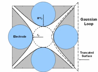
Boumsellek at al. argued that as a quadrupole decreases in size, the capacitance will increase [4] but a simple 2D model can be used to show otherwise. Our model assumes an ideal quadrupole potential established by hyperbolic electrodes that are truncated in the orthogonal directions at a distance D + r0, where D = 2·(ψ ·r0). This choice is to
reflect the geometry of a typical QMF with an aperture radius r0 and an electrode r-to-r0
ratio of ψ. A schematic of our model is shown in Figure 3-2 for clarification. From Gauss’ law, the charge on the electrode surface is
∫
⋅= E dA
Q ε0 r r (3-3)
where ε0 is the permittivity of free space, dAr is the normal area differential, and Er is the
electric field. Taking the Gaussian loop as shown in Figure 3-2, the electric field along the hyperbolic surfaces is
(
)
2 2 2 ˆ ˆ 2 0 0 o r y x y y x x r E = − − − = ∇ − = rφ φ r (3-4) with field lines parallel to dAr, and is assumed to be zero on the truncated surfaces. From our model, the total capacitance of a quadrupole with length L can be approximated by[
]
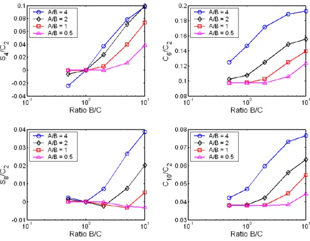
(
)
L L C C r x x r L dx r x r x r L C x r r x r x r x 0 2 * 0 ) 1 2 ( 2 0 2 2 0 0 ) 1 2 ( 2 0 2 2 0 2 2 0 0 0 ] 1 2 8 [ 4 2 4 0 0 0 0 ε ψ ψ ψ ε ε ψ ψ + + = = − = − − = = + = + = =∫
(3-5)Figure 3-2: Model for capacitance calculation
Our model predicts that the device capacitance scales with length, so scaling-down a quadrupole should decrease capacitance. Equation 3-5 implies that the capacitance per unit length is constant and was verified using MAXWELL 2D from Ansoft. Simulations with energy error < 0.1% were utilized to calculate the capacitances of devices with ψ = 1.148 and r0 values ranging between 50 µm and 500 µm. MAXWELLL returned a
capacitance of 2.1 pF/cm while Equation 3-5 gives 3.67 pF/cm. These values are overestimates because they neglect the 3D effects present in quadrupoles with finite length. To get a better estimate of the capacitance, quadrupoles with electrode diameters ranging from 500 µm to 1500 µm, and lengths between 25 mm and 100 mm were simulated with an energy error < 5% in MAXWELL 3D. The average capacitance per unit length was 1.75 pF/cm and was found to be nearly constant for quadrupoles with aspect ratios greater than 100. This value is very close to the 1.67 pF/cm measured for the out-of-plane MEMS quadrupole reported by Velásquez-García [47].
Aside from the device capacitance mentioned, parasitic capacitances also play an important role in the drive electronics. A quick circuit diagram can be used to determine the net capacitance as shown in Figure 3-3. The transformation is accomplished by assuming that the capacitance between adjacent electrodes (Cquad) is comprised of two
symmetric. If we assume that each electrode is identical and the associated parasitic capacitance (Cpara) is also identical, the total capacitance is given by 4Cquad + Cpara. The
quantity 4Cquad should be approximately equal to the quadrupole capacitance given by
Equation 3-5. From this analysis, we see that parasitics can potentially dominate the device capacitance for scaled-down devices (small L) so attention should be paid to minimize them.
Figure 3-3: Device model for parasitic capacitances
Power consumption in the device can be estimated from the formula CV2f/2 where V is given by Equation 3-2, and C is the total capacitance of the device.
Lf r qf e m L C C P para 2 2 0 2 2 * 2 2 1 + = π (3-6)
From Equation 3-6, we see that if the quadrupole length and radius are scaled-down by the same factor that the frequency is increased, effectively maintaining the aspect ratio and performance metrics, the power consumed won’t be significantly affected unless the Cpara/L term dominates. At this point, power consumption will increase as the device
length shrinks. Ultimately, the biggest drain on total system power will still be the vacuum pump.
3.1.3 Pressure
For proper QMF operation, the mean free path of the gas to be analyzed should be larger than the largest dimension of the quadrupole. The reason for this criterion is to ensure that an ion will traverse the length of the device without colliding with another ion or a neutral molecule. The mean free path for air at room temperature is given by
P P d T kB 50 ~ 2π 2 λ = (3-7)
where kB is the Boltzmann constant, T is the temperature, d is the diameter of the gas
molecules, P is the pressure in Torr and λ is the mean free path in microns.
Work on ionizers for the MGA demonstrated a maximum operational pressure around 1 mTorr [40], [41]. This pressure translates to a quadrupole that can’t be longer than 50 mm for proper operation. If higher pressures can be achieved, the vacuum pump will have relaxed pumping requirements, and the detector can be less sensitive. Unfortunately, the quadrupole will need to be shorter, leading to increased drive frequencies and larger voltages if performance is to remain unchanged. Throughout the design process and device characterization, one should be aware of the potential for arcing between the QMF electrodes and plasma formation in the ionizer. This electrical breakdown is dictated by the Paschen curve (Figure 3-4) which plots the breakdown voltage as a function of the operational pressure and the spacing between electrodes.

![Figure 2-5: Non-linear resonances in the first stability region [69]](https://thumb-eu.123doks.com/thumbv2/123doknet/14295250.493228/31.918.209.709.288.650/figure-non-linear-resonances-stability-region.webp)
![Figure 2-6: Upper and lower corners of the second stability region [78]](https://thumb-eu.123doks.com/thumbv2/123doknet/14295250.493228/33.918.144.776.617.899/figure-upper-lower-corners-second-stability-region.webp)