Contributions to the direct time integration in wave propagation analyses

Contributions to the Direct Time Integration

in Wave Propagation Analyses

by

GUNWOO NOH

S.M. Mechanical Engineering

Massachusetts Institute of Technology, 2011 B.S. Mechanical Engineering

Korea Advanced Institute of Science and Technology, 2009 Submitted to the Department of Mechanical Engineering in Partial Fulfillment of the Requirements for the Degree of DOCTOR OF PHILOSOPHY IN MECHANICAL ENGINEERING

at the

MASSACHUSETTS INSTITUTE OF TECHNOLOGY

September 2013

0 2013 Massachusetts Institute of Technology. All rights reserved.

Signature of Author ...

Certified by .. ...

Department of Mechanical Engineering August 10, 2013 ----- - . . . ...

Klaus-Jirgen Bathe Professor of Mechanical Engineering Thesis Supervisor

A ccepted by

...

...

David Edgar Hardt

Professor of Mechanical Engineering

iMSSACHUSETTS

_F

OFTECHNOLOGy

NOV 12 2013

Contributions to the Direct Time Integration

in Wave Propagation Analyses

by

Gunwoo Noh

Submitted to the Department of Mechanical Engineering on August 10, 2013 in Partial Fulfillment of the Requirements for the Degree of Doctor of Philosophy in

Mechanical Engineering

ABSTRACT

This thesis intends to contribute to the computational methods for wave propagations. We review an implicit time integration method, the Bathe method, that remains stable without the use of adjustable parameters when the commonly used trapezoidal rule results in unstable solutions. We then focus on additional important attributes of the scheme. We present dispersion properties of the Bathe method and show that its desired characteristics for structural dynamics are also valuable for wave propagation problems. A dispersion analysis using the CFL number is given and the solution of some benchmark problems show that the scheme is a method for general use for structural dynamics and wave propagations. Finally, we propose a new explicit time integration method for the analysis of wave propagation problems. The scheme has been formulated using a sub-step within a time step to achieve desired numerical damping to suppress undesirable spurious oscillations of high frequencies. With the optimal CFL number, the method uses about 10% more solution effort as the standard central difference scheme but significantly improves the solution accuracy and a non-diagonal damping matrix can directly be included. The stability, accuracy and numerical dispersion are analyzed, and solutions to problems are given that illustrate the performance of the scheme.

Keywords

Direct time integrations, Structural dynamics, Wave propagations, Numerical damping, Numerical dispersion

Thesis Committee Members

Professor Klaus-JIrgen Bathe (Committee chair); email: [email protected] Professor Tomasz Wierzbicki; email: [email protected]

Acknowledgements

I would like to express my deepest gratitude to my advisor, Professor Klaus-Jirgen Bathe,

for his extraordinary guidance, support, and kindness. It has been a truly fantastic experience to work with a brilliant researcher who has a great attitude. It also has been a pleasure to work under this wonderful teacher, who is very patient and always understands and encourages his student. Professor Bathe has been a true educator to me, and this dissertation would not have been possible without his invaluable mentorship.

I also wish to express sincere gratitude to my other thesis committee members, Professors

Tomasz Wierzbicki and Raul A. Radovitzky, for their valuable advice and insights into the work presented herein. Undoubtedly, their suggestions have strengthened the quality of my work. I also deeply appreciate their kind encouragement during my time at M.I.T.

I also thank all my friends in the Finite Element Research Group. I will never forget the

breakfast burritos that we had after overnights in our office, the jokes we used to tease each other with in our own language, and the beers we had for no reason, although their advice on my research may have been of less importance. It is also impossible to imagine my graduate life without my friends in MIT MechE, KGSA-ME and the KGSA basketball team.

They all made my time at M.I.T. very special.

I also deeply appreciate the Samsung Scholarship Foundation for their generous financial

support for the last four years.

Finally, and most importantly, I offer my most valuable appreciation to my family for their unconditional support and endless love. Without them, I would have very little today. I am

Contents

2.1. The basic equations of the Bathe method... 17

2.2. The stability and accuracy properties... 21

2.3. A demonstrative solution...26

2.4. Concluding remarks ... 34

Chapter 3 On an implicit time integration scheme in the analysis of the wave propagations ... 36

3.1. A dispersion analysis ... 36

3.1.1. A dispersion error analysis in the ID case... 39

3.1.2. A dispersion error analysis in the 2D case... 45

3.2. Wave propagation solutions... 53

3.2.1. 1-D bar impact ... 53

3.2.2. 2-D scalar wave propagation ... 60

Chapter 4

A new explicit time integration scheme for wave propagations ... 73

4.1. An explicit time integration scheme ... 73

4.1.1. Stability and accuracy characteristics... 76

4.1.2. A dispersion error analysis for 2D case ... 84

4.1.3. Selection of load magnitude at substep ... 94

4.2. Wave propagation solutions...98

4.2.1. 2D scalar wave propagation ... 98

4.2.2. Wave propagations in a semi-infinite elastic domain... 105

4.3. C oncluding R em arks ... 111

Chapter 5 Conclusions ... 113

References ... 115

Appendix ... 120

A. 1 Effect of splitting ratio, "Y in the Bathe method ... 120

A.2 On the solution of the Bathe method for a model problem ... 123

A.2.1 Desired solution: mode 1 + static correction... 123

A.2.2 Solution from the Bathe method... 124

A .2.3 C om parisons ... 126

A.3 On numerical wavelength and phase speed with respect to the time step size 131 A.4 Integration approximation and load operators of the proposed method... 136

List of Figures

Figure 2-1 Spectral radii of approximation operators, case = 0, for various methods.... 23

Figure 2-2 Percentage period elongations for various methods... 25

Figure 2-3 Percentage amplitude decays for various methods... 25

Figure 2-4 Model problem of three degrees of freedom spring system ... 26

Figure 2-5 Displacement of node 2 for various methods ... 28

Figure 2-6 Displacement of node 3 for various methods ... 28

Figure 2-7 Velocity of node 2 for various methods... 29

Figure 2-8 Velocity of node 3 for various methods ... 29

Figure 2-9 Acceleration of node 2 for various methods ... 31

Figure 2-10 Acceleration of node 2 for various methods ... 31

Figure 2-11 Acceleration of node 3 for various methods ... 32

Figure 2-12 Reaction force at node 1 for various methods... 33

Figure 2-13 Reaction force at node 1 for various methods... 33

Figure 3-1 Relative wave speed errors of the Bathe method for various CFL numbers... 44

Figure 3-2 Relative wave speed errors of the trapezoidal rule for various CFL numbers ... 44

Figure 3-3 Relative wave speed errors of the Bathe method for various propagating angles, for CFL = 1 for various effective fundamental length, L... 51

Figure 3-4 Relative wave speed errors of the trapezoidal rule for various propagating angles, for CFL = 0.65 for various effective fundamental length, L... 52

Figure 3-5 1D bar impact problem ; co = 5000 ... 54

Figure 3-6 Velocity distributions from the Bathe method for various CFL numbers... 56

Figure 3-7 Velocity distributions from the trapezoidal rule for various CFL numbers... 56

Figure 3-8 Acceleration distributions from the Bathe method for various CFL numbers.. 57

Figure 3-9 Acceleration distributions from the trapezoidal rule for various CFL n u m b ers ... 5 7 Figure 3-10 Velocity distributions for various observation times ... 58

Figure 3-11 Acceleration distributions for various observation times ... 59

Figure 3-13 Snapshots of displacements at t = 13, Trapezoidal rule, CFL = 0.65... 62

Figure 3-14 Snapshots of displacements at t = 13, Bathe method, CFL = 1... 63

Figure 3-15 Displacement variations along the various propagating angles ... 64

Figure 3-16 Velocity variations along the various propagating angles... 64

Figure 3-17 A Lamb problem. Vp = 3200, Vs =1848, V =1671... 66

Figure 3-18 Time history of displacement variations in x-direction and y-direction at the two receivers on the surface; Ricker wavelet line load ... 68

Figure 3-19 Snapshots of von Mises stress; Ricker wavelet line load ... 69

Figure 3-20 Time history of displacement variations in the x- and y-directions at the two receivers on the surface; step functions line load ... 70

Figure 3-21 Snapshots of von Mises stress at t = 0.9196 s; step functions line load... 71

Figure 4-1 Spectral radii of approximation operator, case = 0, of the proposed explicit m ethod for various values of p... 81

Figure 4-2 Percentage period elongation and percentage amplitude decay of the proposed m ethod for various values of p ... 83

Figure 4-3 Spectral radii of approximation operators, case = 0, for various methods; for the proposed explicit scheme, p = 0.54 is used ... 84

Figure 4-4 Relative wave speed errors of the proposed method for various CFL numbers; usin g p = 0 .54 ... . 92

Figure 4-5 Relative wave speed errors of the central difference method for various CFL n u m b e rs... 9 2 Figure 4-6 Relative wave speed errors of the proposed method for various propagating angles, using CFL = 1.85 and p = 0.54 ... 93

Figure 4-7 Relative wave speed errors of the central difference method for various propagating angles, using CFL = 1 ... 93

Figure 4-8 Pre-stressed membrane problem, co =1 , initial displacement and velocity are zero, com putational domain is shaded ... 99

Figure 4-9 Snapshots of displacements at t = 9.25, Central Difference method,

Figure 4-10 Figure 4-11 Figure 4-12 Figure 4-13 Figure 4-14 Figure 4-15 Figure 4-16 Figure 4-17 Figure 4-18 Figure 4-19 Figure Al-i Figure A1-2 Figure Figure Figure Figure A3-1 A3-2 A3-3 A3-4

Snapshots of displacements at t = 9.25, Proposed method, CFL = 1.85,

p = 0 .5 4 ... 10 1

Displacement variations along the various propagating angles, at time t = 9.25, 88 x 88 elem ent m esh ... 102

Velocity variations along the various propagating angles, at time t = 9.25, 88 x 88 elem ent m esh ... 102

Displacement variations along the various propagating angles, at time t = 9.25,

132 x 132 elem ent m esh ... 103 Velocity variations along the various propagating angles, at time t = 9.25,

132 x 132 elem ent m esh ... 103

A Lamb problem. V = 3200, Vs = 1848, Vyeig =1671... 105

Time history of displacement variations in x-direction and y-direction at the two receivers on the surface; Ricker wavelet line load ... 107

Snapshots of von Mises stress at t = 0.9828 s; Ricker wavelet line load ... 108

Time history of displacement variations in x-direction and y-direction at the two receivers on the surface; line load of step functions ... 109 Snapshots of von Mises stress at t = 0.9828 s; line load of step functions... 110

Spectral radii of approximation operator of the Bathe methods. The fraction factor - is given in the parentheses... 121

Percentage period elongations and percentage amplitude decays of the Bathe methods. The fraction factor is given in the parentheses. ... 121

Relative wavelength errors of the Bathe method for various CFL numbers.... 132 Relative wavelength errors of the Trapezoidal rule for various CFL

n u m b e r s ... 1 3 2 Relative wave speed errors of the Bathe method for various CFL numbers... 135 Relative wave speed errors of the Trapezoidal rule for various CFL

List of Tables

Table 2-1 Step-by-step solution using the Bathe integration method ... 20

Table 4-1 Step-by-step solution using the proposed method for linear analysis with general lo a d ing ... 9 7

Chapter 1

Introduction

In the solutions of structural dynamics and transient wave propagation problems, direct time integration with finite elements is widely used and can be categorized into two groups: explicit and implicit methods. The method is explicit unless the solution procedure requires factorization of the "effective stiffness" matrix, in which case it is implicit [1-3].

In general, each method type has its own advantages and disadvantages. Implicit methods can be designed to have unconditional stability, so that the time step size can be selected solely based on the characteristics of the problem at hand. However, implicit methods require much larger computational costs per time step than explicit methods do, since explicit methods can be designed to require only vector calculations with the diagonal mass matrix. However, an explicit method can only be conditionally stable. Hence, explicit methods can be very effective when the time step size required by the stability limit is either greater than or not much less than that required to describe the problem, as in wave propagation analyses, for example [1-5].

deteriorate due to dissipation and dispersion errors, which are caused by spatial and temporal discretization [1]. Spurious oscillations, especially for high wave numbers, ruin the accuracy of the solution [6-11]. These oscillations are from dispersion error, which is also related to Gibb's phenomenon or pollution effect. As a wave travels, the errors from the difference between numerical wave velocities and physical wave velocity accumulate, also affecting the dissipation error by dispersing the wave, whereby the solution becomes more erroneous.

Hence, there has been a considerable effort to reduce the dispersion errors. First, by improving spatial discretization, dispersion errors can be reduced. Most straightforwardly, a fine.mesh with a very small time step size can be used. This strategy requires that the time step be selected carefully, depending on the element size; otherwise, the solution errors remain large, even with a fine mesh [1, 12, 13]. Different types of higher-order spatial discretization [14-24] may be used to improve the solution accuracy. However, the use of higher-order spatial discretization can be very computationally expensive and may not have the generalizability of the traditional finite element procedures using low order elements.

The errors from spatial and temporal discretization appear concurrently, and they affect each other in the solutions of transient wave propagation. Dispersion errors from spatial discretization, temporal discretization, and the coupled influence of both discretization errors have been analyzed for some cases [25-30]. Analyses of these errors have led to the

use of linear combinations of consistent and lumped mass matrices [26, 31-35]. By balancing the effect of the consistent and lumped mass matrices, these approaches may considerably reduce the dispersion error in one dimensional analysis. However, by this technique alone, good accuracy in general higher dimensional wave propagation problems is difficult to achieve.

Other approaches have been introduced to minimize dispersion errors. These use the mass and stiffness matrix from the modified integration rule [30, 35, 36] and shift the numerical integration points from conventional Gauss or Gauss-Lobatto integration points in the calculation of mass and stiffness matrices. However, different integration rules than those commonly used have been proposed, and these rules may also depend on the material properties, which renders these approaches impractical.

To improve the solution of wave propagation problems, another category of approaches have been introduced that filters the resulted spurious modes. First, to minimize spurious oscillations by pre/post-processing, a digital filter [37] and time integration for the filtering stage [35, 38] have been introduced. However, the filters are only applicable to specific points in space and time. Hence, these techniques do not lend themselves to analyses requiring a solution for all times and over the complete solution domain, for example, for making a movie of the calculated displacements and stresses.

Numerical dissipations are used in many direct time integration methods to improve the solution by suppressing high frequency spurious wave modes [1, 2, 39, 40]. Using this strategy, accurate solutions are difficult since the introduced numerical dissipation should be large enough to suppress the high frequency spurious waves, while good accuracy for the low frequency waves should be simultaneously ensured. However, this approach can be very effective since the solution procedure does not require any additional computational cost and can be used for structural dynamics and wave propagation problems in a uniform manner.

A number of implicit time integration methods have been proposed, the trapezoidal rule and

the alpha methods are now being the most commonly used [1, 41]. As is well known, the trapezoidal rule is unconditionally stable in linear analysis, second-order accurate, and, regarding time integration errors, shows no amplitude decay and acceptable period elongation [1]. However, the dispersion errors in the high frequency modes may ruin the solutions significantly in the wave propagation analysis since the trapezoidal rule is non-dissipative. Moreover, the method may become unstable in nonlinear analyses, in which case momentum and energy are clearly increased. Hence, researchers have sought more effective time integration schemes.

To introduce some damping into a time integration method, adjustable parameters are employed, and this approach has been used in the design of the alpha methods [41]. In these methods, the parameters have to be selected based on the characteristics of the problem

solved. Since inappropriate parameters may result, adjustable parameters itself may render the approach ineffective.

Recently, the Bathe method [42-44] has been presented and shown to result in remarkably accurate solutions by having damping properties to limit the solution error for physical wave modes, and by almost discarding the high spurious modes [45]. With its optimal CFL number, the method results in very small numerical dispersion error in all the participating wave modes by practically eradicating the high spurious modes, which cannot be well represented spatially. Furthermore, the capabilities in structural dynamics and unconditional stability render the Bathe method very attractive as a general method for structural dynamics and wave propagation problems [42-46].

Among explicit methods, the central difference method is still the most widely used scheme. It has the highest stability limit of any second-order accurate explicit method [47, 48]. The central difference method uses a matrix factorization for systems with a non-diagonal damping matrix [49, 50]. However, since the central difference method is a non-dissipative method, the solution accuracy can be ruined by the dispersion errors in the high frequency modes.

The development of dissipative explicit methods has been heavily pursued [51], and schemes have been presented by Newmark [52], Chung and Lee [3], Zhai [53], Hulbert and

explicit method, and the Zhai explicit scheme with high-frequency dissipation are only first order accurate, and the latter two decrease the solution accuracy in the low frequency domain.. Comparative studies [55, 56] show that the remaining dissipative explicit methods are second-order accurate but often provide less accurate solutions than the Tchamwa-Wielgosz method.

This thesis presents a study of the Bathe method for structural dynamics and wave propagation problems, demonstrating that the characteristics that the Bathe method possesses are valuable, and then presents a novel and improved explicit time integration method for wave propagation analysis. In Chapter 2, the characteristics of the Bathe method in linear structural dynamics are reviewed and discussed. In Chapter 3, the properties of the Bathe method in the solution of wave propagation problems are analyzed. In Chapter 4, based on Chapters 2 and 3, a new explicit time integration method for wave propagation for significantly improved solutions is proposed. We note that most of the presented content in this thesis is similar (and in parts identical) to that published in their previous papers [44, 45, 57]

Chapter 2

A review of an implicit time integration

scheme in structural dynamics

This Chapter comprises a study of the Bathe method in structural dynamics, comparing its performance with the trapezoidal rule and two additional members of the Newmark family of methods that may be considered for solutions. First, the basic equations of the Bathe are briefly reviewed and some basic properties of the time integration method are presented. Then, the scheme is applied, along with the other methods, in the solution of a simple linear "model problem" to illustrate some important and valuable properties of the method, increasing insight into the method [44].

2.1.

The basic equations of the Bathe method

The governing finite element equations, in linear analysis, to be solved are

with initial conditions where U and R are the nodal values of the solution and the vector of externally applied nodal forces, and M, C, K are the mass, damping and stiffness matrices, respectively. The time integration scheme obtains the solutions at time t +At using some previously calculated solution variables up to time t, with the predefined time step size At.

In the Bathe method, the complete time step At The trapezoidal rule is used in the first sub-step, Euler backward method is employed. The resulting

consists of two equal-length sub-steps. and in the second sub-step the 3-point equations are (2.2) (2.3) (2.4) t+At/2 _{t + t+&/20} 4

tt2 _{U='U + At ('U+ I+A/2Uj)}

,

1 4

t+At _{1-U - 4 t+At/}2

U+ - t+U, At At At 0 _{-t- 4 t+&1}2 _fj + ' t+Afj At At At (2.5) and

Equations (2.2) to (2.5), with the equilibrium at time t + At /2 and t + At, result in the time-stepping equations as

16 + C+K t+At/2U = t+A/2 ,

At2 At

)

t+At/2g A I+At/2R M( 16 'U+ I 'U+' + +C 4 'U'U,

At2

At _{( AtcU+t0}

t+AtI9 t+AtI2R ± M+A

CA6t

3

9 3

(

+C 4

)

Eqs. (2.6) and (2.8) are used successively for each time step to solve for the required solution over the complete time domain considered with the initial conditions corresponding to initial time known. Prior to the time integration, a time step At is defined, and the "effective stiffness matrices" defined in Eqs. (2.6) and (2.8) are factorized. For each time step, the calculation of the effective load vectors and forward-reductions and where

Table 2-1 Step-by-step solution using the Bathe integration method

A. Initial calculation

1. Form stiffness matrix K , mass matrix M, and damping matrix C 2. Initialize U, I and

U.

3. Select time step At and calculate integration constants:

16 4 9 3

a- 2' a==-; a₂ - a

=-At At At At

12 a 3 1

a4 = 2a; a =- At2' a7 At

4. Form effective stiffness matrices K1 and K2:

KI =K+aoM+a₁C; K2=K+a2M+a3C

5. Triangularize K1 and K Ki = L D Lj; K2= L2D2L .

B. For each time step:

<First sub-step>

1. Calculate effective loads at time t + At / 2: St 2_{R + M(aO}

U + a4 'jJ +t) + C (a'U+'U) 2. Solve for displacements at time t + At /2:

LDLI t+Ati2U =t+At2

3. Calculate velocities at time t + At / 2:

t+At2 = aI (+AI 2U -'U) -'U 4. If required, evaluate accelerations at time t + At / 2:

t+At/2U _{= ai(t+A}2 _U

-'U) -'U <Second sub-step>

1. Calculate effective loads at time t + At:

tAt _{R + M(a 't/2U+ a'U+ a'+At/2U+a'U) + C (a t+At/2U a,'U)} 2. Solve for displacements at time t + At / 2:

L2D2L t+AtU = t+At

3. Calculate velocities and accelerations at time t + At /2:

t+t ₇t_{u _aa t+AN}2

U+a3+ U

The same effective stiffness matrix in Eqs. (2.6) and (2.8) may be advantageous to use in linear analysis. The same effective stiffness matrix is achieved by using the value

(2-

vU2)

l)At

factorization of an effective stiffness matrix is required. In addition, less memory is needed if the matrix can be kept in-core.

On the other hand, in nonlinear analysis, the use of the different effective stiffness matrices in each sub-step does not increase the solution effort. This is because, in nonlinear analysis, Newton-Raphson iterations are used with new tangent stiffness matrices in each iteration. The resulting solution procedure of the Bathe method is summarized in Table 2.1.

2.2.

The stability and accuracy properties

Some properties of the method can be analyzed through the following equation [1]:

[t±At

t~

t+At = t' i +Lat+A1'r+Lbt'At'r 2 , (2.9)

t+At t d

-4wAt(24 + 7cAt) -4At(-12 + W2At2) 4At2_{(7+ 2 coAt)} +1(-288 +14{ 2_At2 -144wAt + 5_)At3 3 _{+ 48} 2coAt) 14 - CO 2At2 - 8 c3At'3 - 24{wAt At(144-5 2_At2 _{+80{At +16 2w2 At}2₎ C2 _{(245wAt + 19w}2 At2 _-144)

C2At(-96 - 245wAt + 2A2) 2

-19 2 At2 _{+ 144 + 168 cAt + 48$2} 2_At2 _-25c3At3 -4ctAt(24 + 7coAt) La =

A8

pA

co and are the natural frequency and the damping ratio, respectively. The spectral radii of various methods for case = 0 are shown in Fig. 2-1.

(2.10)

(2.11)

(2.12)

with

p(A) 0 0 0 0 1V 10- 10- 100 10 102 10* At / To

Figure 2-1 Spectral radii of approximation operators, case = 0, for various methods;

p(A)=1.0 for the Newmark trap. rule and when a =1/2,5=1/2 in the Newmark method

The equations used in the Newmark schemes are [1]

(2.14)

U+Ii

'j+ [(I-8)'U +,5'1+Ut At

and

t+A U='U+'tAt+ (--a) ' +a '+AJ At2

w

2

where the parameters a and 9 used are given in Fig. 2-1.

(2.15)

An important point is that the Bathe method gives the value of p(A) almost 1.0 up to At / T 0.1, and the value rapidly decreases thereafter. This shows a very desirable

.8

.6-- _Bathe

- Euler 3-point backward

Houbolt .2 - Wison (9 = 1.4)

- Newmark (trap. rule)

Newmark (a =1/2, 8 = 1/2) Newmark (a = 3/10, = 11/20) 1

property of time integration since it indicates unconditional stability, highly accurate integrations up to At / T is 0.1, and, thereafter, strong numerical damping in the response for which At / T is larger than about 0.3. It is observed that the use of 2- NT instead of 1/2 for the splitting of the time step results in practically the same curve of p(A). The properties of the method for the various splitting ratios are discussed in Appendix Al.

The amplitude decays and period elongations are shown in Figures 2-2 and 2-3, respectively, which show the accuracy properties of the scheme. Very small amplitude decay and period elongation are observed in the Bathe method for reasonable time step values. For example, the solution accuracy for period calculations in the Bathe method with

At / T = 0.1 is similar to that of the trapezoidal rule with At / T = 0.07.

Moreover, the numerical damping shown by its spectral radii (Fig. 2-1) results in improved stability characteristics in nonlinear analyses [42, 43]. Section 2.3 presents a discussion of the importance of this numerical damping, which is very small for reasonable At / T values and is large for large At / T values, in linear structural dynamics analysis.

351_1_1_ _ C 0 cc Cn C 0 w 0 0-4) 0) cc 4) 0 30 F 25 20 15 10 5 0 0 0.05 0.1 0.15 0.2

Figure 2-2 Percentage period elongations for various methods

30f C 0 25 0 20 0 15 (D CD a. 5 0 0 0.05 0.1 At / TI) 0.15 0.2

Percentage amplitude decays for various methods; results for Newmark (trapezoidal rule) and Newmark (a =I / 2, t =1 / 2) are identical

- Bathe

- Euler 3-point backward

Hiouoi

- Wilson (e = 1.4)

- Newmark (trap. rule)

Newmark (a =1/2, 8 = 1/2) - Newmark (a = 3/10, 8 = 11/20)

- Bathe

- Euler 3-point backward

MOUDOIT

- Wilson (0 = 1.4)

- Newmark (trap. rule) Newmark (x =1/2, 8 = 1/2)

- Newmark (a = 3/10, 8 = 11/20)

2.3.

A demonstrative solution

This Section considers the solution of a simple three degree-of-freedom spring system, as shown in Fig. 2-4, to deepen insight into the Bathe method. Since the prescribed displacements are applied on node 1 over time, as given in Figure 2-4, the governing

equation for the unknown displacements u2 and u3 is

[M2 0]

[Z:]

EU2]

[kIUI], _(2.16)

0 M3 i3 _-k2 _k2 .U3 ₀

where the reaction becomes

A = MAu +kAu - kIU2 .(2.17)

Ri

U1

Figure 2-4 _{Model problem of three degrees of freedom spring system}

k, =107, k2 =1, mI =0, m2 =1, m3 =1, o, =1.2

Note that this very simple problem is used as a "model problem" to represent a much more complex structural system that includes the stiff and flexible parts. For example, the left

very stiff spring in the model problem represents almost rigid connections or penalty factors used, while the right flexible spring is used to represent the flexible parts of the complex structural model.

An important point is that the almost rigid parts in the complex model, which are frequently idealized by artificially stiff truss or beam elements, play an important role; however, the detailed response within these parts should not frequently be included in the overall system response. This is because, in practice, the highly stiff parts have often no physical meaning, simply being used to provide constraints. Hence, a response that corresponds to very high artificial frequencies would not be included in a mode superposition analysis.

The stiff spring could be idealized as a rigid link reducing the system to only two degrees of freedom. However, in practice, such stiff elements are varied in many parts of complex finite element models and may not be reducible. The system in Fig. 2-4 is used as a "model system" to study the behavior of the numerical solution for such complex structural systems when obtained by the direct integration schemes.

As must typically be done in a complex many degrees-of-freedom structural analysis, zero initial conditions for the displacements and velocities at nodes 2 and 3 are used, and the system is solved for the response over 10 seconds. For the solution, the time integrations are applied to Eq. (2.16), and the reaction is calculated using Eq. (2.17).

-e- _{Newmark (trap. rule)} 2 Newmark (a=1/2, 6=112) + Newmark (a=3/10, 8=11/20) 1.5 -- Bathe - reference

1-UAt2

Figure 2-5 Displacement of node 2 for various methods

4

-e- Newmark (trap. rule)

Newmark (a=1/2, 8=1/2) 3 --- Newmark (a=3/10, 8=11/20) -4- Bathe - reference 2-U3 2 -' 4 6 8 10 time

4 -- 8- Newmark (trap. rule) Newmark (a=1/2, 8=1/2) -- Newmark (a=3/10, 8=11/20) 3 - -- Bathe -- reference 2 -U21 -2-0 2 4 6 8 10

time

Figure 2-7 Velocity of node 2 for various methods (the static correction gives the nonzero velocity at time = 0.0)

4

-e- Newmark (trap. rule)

3- Newmark (a=1/2, 8=1/2) -0- Newmark (a=3/10, 6=11/20) -e- Bathe 2 - reference U3 -2--3 -4--5 0 2 4 6 8 10

time

In addition, the time step used is At = 0.2618; therefore we have At

/

At

/

the system in Eq. (2.17) and the period of the prescribed motion at node 1, respectively.

The calculated solutions are given in Figures 2-5 to 2-13. In these figures, we also give a "reference solution," which is obtained in a mode superposition solution, using only the lowest frequency mode plus the static correction as is typically done in a practical analysis for a many degrees-of-freedom model (of course, in practice, the number of low frequency modes used depends on the problem at hand) [1].

The calculated responses given in the figures indicate that the Bathe method performs very well while others provide inaccurate solutions, in particular for the acceleration at node 2 and the reaction. The trapezoidal rule shows "practically" instability in the calculation of the reactions and accelerations, (see Fig. 2-12). On the other hand, the Bathe method calculates the solutions very accurately without the adjustment of any parameter. Only for the first time step is there an "undershoot" as shown in Figs. 2-10 and 2-13 while, of course, this undershoot can also be removed by setting the initial conditions to excite only the physical mode. (See Appendix A2 for details). The important point to note is that the method performs as a mode superposition analysis is performed: it does not include the high frequency mode to the total responses, which is artificial due to modeling, so that the calculated response becomes accurate.

800 -

--G Newmark (trap. rule)

60- Newmark (a=1/2, 6=1/2) -e- Newmark (a=3/10, 8=11/20)

--" Bathe 400 - reference 200 -2 0 -200 -400 -600--800 -_-0 2 4 6 8 10

time

Figure 2-9 _{Acceleration of node 2 for various methods}

25 - - -Newmark (a=1/2, 6=1/2) 20- -- Newmark (a=3/10, S=11/20) -0- Bathe 15 --- reference 10 -.. 5 U2 -5 -10 -15--20- --25-II S2 4 6 8 10 time

-e- _{Newmark (trap. rule)}

Newmark (cc=1/2, 6=1/2)

3 - e-- Newmark (a=3/10, S=11/20)

-e- Bathe 2 -- reference U3 -2- -3--0 2 4 6 8 10 time

Figure 2-11 Acceleration of node 3 for various methods

This feature of the method is valuable for practical analyses, and valid for both linear and nonlinear analysis. Only a simple model problem was considered in order to focus on the essence of the characteristics of the method; however, the same conclusions can be applied solving a large finite element models in practical analysis.

80 600 400 200 -200 -400 -600

-e- Newmark (trap. rule Newmark (a=1/2, 8 - Newmark (a=3/10, -e- Bathe - reference - M - - - - - - - - - - - - - --8000L 0 2 4 =1/2) 6=1 1/20) time 6 8

Reaction force at node 1 for various methods

4

time 6 8 10

Reaction force at node 1 for various methods

Ri

10

I Newmark(ct=1J2.~=1I2~ _I -e- Newmark (a=3/1 0, S=11/20)

-+- Bathe - reference Figure 2-12 25 20 15 10 5 -5 -10 -15 -20[ -25' 0 Figure 2-13 2 n I

-2.4.

Concluding remarks

Complex finite element systems with flexible and very stiff parts are frequently used in practice, where the stiff part may only model constraints. In solutions with appropriately chosen time step size, the direct time integration methods are used for all coupled degrees of freedom over the time domain.

In this Chapter, the performance of the Bathe method is studied for structural dynamics. In particular, to represent the essence of such complex flexible/stiff systems, we considered a

simple two degree-of-freedom "model problem" to study the numerical solutions using the trapezoidal rule, two other direct time integration schemes from the Newmark family of methods, and the Bathe method.

The response from the Bathe method was obtained as in a mode superposition analysis. Numerical damping properties in the Bathe method damped out the artificial high frequency modes so that it is not included as errors in the solutions. As is desired in practice, only the physical mode that is excited is accurately included in the response together with the static correction in the solution of the Bathe method.

On the other hand, the other methods used, and in particular the trapezoidal rule, provided inaccurate solutions. Although numerical damping is included in one Newmark method, the solution errors are large.

Here, to focus on the essence of desired properties of time integration in structural dynamics, the study was deliberately limited to not include time integration techniques for which numerical parameters need to be chosen, such as the alpha-method [41]. We believe that the simple "model problem" considered in this Chapter would be valuable to analyze the other procedures for structural dynamics.

Chapter 3

On an implicit time integration scheme in

the analysis of the wave propagations

In this Chapter, the Bathe method for wave propagation problems is discussed, and it is shown how the desired properties for structural dynamics can also be valuable for wave propagation problems. Dispersion properties of the Bathe method and the trapezoidal rule with linear spatial discretization for 1 -D and 2-D cases are studied. Based on the dispersion analysis, it is demonstrated that the scheme's properties, which are valuable for structural dynamics, can be valuable for wave propagations; subsequently, the performances of the scheme, with the trapezoidal rule, are evaluated through numerical examples.

3.1.

A dispersion analysis

This Section offers an analysis of dispersion errors resulting from spatial discretization coupled with temporal discretization of the Bathe method and the trapezoidal rule. These

dispersion errors can be analyzed by employing the scalar wave governed by

a2u

t

_V

_u

where u is the field variable and c, is the wave velocity. Here, the main consideration is the dispersion associated with the propagations of disturbances; therefore, body forces are not considered. The associated finite element approximation system gives

Mt+c KU= 0, (3.2)

where K and M are the stiffness and mass matrices, and for element (m) with volume

M(M) =

f

KC") = f,(.) (VHm) )T (VH(m)) dV(m),

(3.3)

(3.4)

and H(m) and U are the shape function matrix and the discretized field variable,

Eqs. (2.2)-(2.5) with Eq. (3.2) at time t , t + At / 2 and t + At can be rewritten in a linear multistep form representing the Bathe method as

(72M

+(72M+5c At2K)tu=0. (3.5)

c0At

Using the definition of the CFL number, CFL = 4, where h is the "characteristic

h

length" of a finite element (or fundamental length used) [1], Eq. (3.5) becomes

(72M + 8YK)'±I'U + (-144M + 57K)t+AN2U

+(72M+5 7K)'U = 0, (3.6)

where y = CFL2 _h2_.

For the Newmark method, using the equilibrium at time t - At, t and t + At, and Eqs.

(2.14) and (2.15), and the same equations for the solution at time t, we get the linear multistep form of the Newmark method (for the case S = 1/ 2) as

(M + ac At2K)''U + (-2M+ (1- 2a)c At2K) U +(M+ac At2K)'-"U =0

or

(M+ ayK)'±U + (-2M + (1- 2a)y K)U

+ (M + ayK) 'T_{U = 0.}

With a =1/ 4, the equations for the Newmark trapezoidal rule are obtained. The above

equations may indicate that the computational cost in the Bathe method is twice that used in the Newmark method, since in the Bathe method, the solution at the half step is used; however, as demonstrated in Section 3.2, this is not the case when solutions of optimal accuracy are sought.

3.1.1. A dispersion error analysis in the ID case

The general solutions of Eq. (3.1) have the form of A el(kox"t) in the 1 -D case, where co

is the frequency of a wave mode and ko = coo / co is the corresponding wave number. A wave mode of an approximated system takes the form [30]

(3.9) ',u = Ake' (k-o')

(3.7)

where c> and k = co / c are the approximated (numerical) frequency and the corresponding wave number, respectively. The approximated wave speed c is different from the exact wave speed co. In addition, the difference is a function of the wave number; therefore, this difference results in artificial dispersion. In addition, for unconditionally stable implicit methods, the amplitude of the numerically calculated wave typically decreases due to its numerical damping [1]. The Newmark trapezoidal rule is an exception since the scheme does not possess any numerical damping. In the following Sections, it is demonstrated that the damping properties in the Bathe method enable remarkably accurate

solutions.

Considering a regular mesh with nodes equally spaced by Ax along the x axis, the solutions to the approximated system at time t + nAt and location x + nxAx become

ntAt k ei(knxAx-wnAt)

k eikAx(n,-n(CFL)(c/co)) (3.10)

where the subscript and superscript denote the nodal value at nAx and time nAt.

finite element equations are (2 1 MAx0 M=- 0 6 . ,0 1 -l 1 K = 0 0 4 1 ... 0 -1 0 ...

0

An implicit relation can be obtained between CFL, c / co , wave number k , and the element size Ax of the Bathe method by substituting Eqs. (3.10)-(3.12) into Eq. (3.6) with

h = Ax and looking into an equation associated with a middle node. The dispersion error with respect to the wavelength A and the element size used are given in Fig. 3-1. See Appendix A.3 for discussion of numerical wavelength and phase velocity with respect to the time step size.

An important point is that there is no CFL number that makes every wave mode have the same wave speed. This can be demonstrated as follows. After taking Taylor expansion on and

(3.11)

polynomial expression of the relative wave speed error is obtained as

c-c_ _{_ 1 (41CFL2 - 48)(kAx)}2 ₊

1 ₍

CO 1152 13271040 . (3.13)

(28363CFL4 - 59040CFL2 _{+ 6912)(kAx)}4 _+0((kAx)6)

From Eq. (3.13), wave modes with kAx <1 can be rendered almost non-dispersive with

CFL = v48 /41; otherwise, it is dispersive for these modes. However, since the shortest

wave length is 2Ax, there are wave modes with kAx >1. For CFL = 148 /41, the wave modes with shorter wave lengths are dispersive (Fig. 3-1). Therefore, there is no CFL number which makes all modes non-dispersive.

However, in the Bathe method, the wave modes with At / T > 0.3 are, in essence, discarded in the total solution (Fig. 2-1 and Chapter 2). Using the definition of the CFL number, kAx is rewritten as

kAx 2c 1 At (3.14)

,z c CFL T

becomes c / co ~1, it can be seen that wave modes with kAx

>

participating wave very accurately.

For the Newmark method, using Eqs. (3.10)-(3.12) and (3.8), and looking into an equation associated with a middle node, the relation between CFL, c / co , wave number k , and the element size Ax is obtained (Fig. 3-2). After taking Taylor expansion on the relation with respect to kAx, the following is obtained:

c - cO 1 1 +

(1-2a)

c_ 24 1920 (3.15)

+(-120a + 9 + 720a2)CFL4)(kAx)4 + 0((kAx)6)

For a =1/ 4, wave modes with kAx <1 become almost non-dispersive with CFL = fI2.

However, wave modes with kAx >1 are dispersive (Fig. 3-2). Therefore, as in the Bathe method, there is no CFL number that makes the solution from all participating wave modes non-dispersive; however, unlike the Bathe method, the trapezoidal rule does not eliminate the dispersive modes from the solution. Hence the solution will generally show a significant

-0.3 0.4 0.5 -0 0.1 0.2 0.3 0.4 0.5 0.6 0.7 0.8 0.9 1 Ax A /2

Figure 3-1 Relative wave speed errors of the Bathe method for various

Discarded wave modes are presented in dashed lines

CFL numbers; 0.3- 0.2-0.1 a -0.1 -0.2 -0.3 -0.4 -0.5 0 0.1 0.2 0.3 0.4 0.5 0.6 0.7 0.8 0.9 1 Ax A /2

Figure 3-2 Relative wave speed errors of the trapezoidal rule for various CFL numbers

0 0 0 -0. -0. .3 CFL = 0.2 -CFL = 1 2 -CFL = .4T841 -CFL = 2 2 CcO CO -0.6 CFL = 0.2 -CFL = 0.65 - CFL = 1/V\ -CFL = 2 C-cO CO -0.6

3.1.2. A dispersion error analysis in the 2D case

The general solution of Eq. (3.1) in 2-D analyses for a plane wave is given by

u = Ae'(cos"O)+kOysi"C")-wO'), and the corresponding numerical solution is

(3.16)

x,y k= (kxcos()+kysin()-ot)

Considering a mesh with nodes equally spaced at distance h along both x and y axes (Ax = Ay = h), the solution of the finite element system at time nAt and location nxh,

nyh becomes

n₁At -A_ _ i(knhcos(8)+knyhsin(9)-orntAt) nh, nyh

-A ke kh(nx cos(9)+n, sin(0)-n, (CFL)(c/co))

(3.17)

where 0 is the angle from the x-axis at which the wave is propagating.

Similar to the 1 -D case, after substituting the above expression of approximated solution into the linear multistep formula, and looking into the equation associated with a middle node, the implicit relation between CFL = c0At / h, c / co , wave number k , and the

For the four-node element, the row of the global mass matrix corresponding to the middle node at (x,y) is

h [0...0 1 4 1 4 16 4 1 4 1 0...0]

36 (3.18)

Therefore, the M'U term for the node at (x,y) is

36 [16 u+ 4( u x+hj) ± xIi, +h ) (3.19)

+( x-hy-h x+h,y-h x-h,y+h + x+h,y+h

u)]

Also, the corresponding row of the global stiffness matrix K is

- [0...0 -1 -1 -1 -1

3 8 -1 -1 -1 -1 0...O]0

Therefore, the K'U term for the node is

1 t

- [8,' U-(,_h, +x+hy XY-h +Xy+h

Sx-h,y-h x+h,y-h x-h,y+h x+h,y+hU)]

(3.20)

Using Eqs. (3.17), (3.19), (3.21) and (3.6), we get an implicit relation between

CFL = coAt / h, c /co, wave number k , and the element size h for the Bathe method,

and the results of various propagating angles with CFL = 1 are shown in Fig. (3-a). As in the 1-D case, no CFL number exists which makes every wave mode have the same wave speed. After taking Taylor expansion on the explicit relation, we get the following polynomial expression. c C-- ₁ (96(cs2 _9-cos 4 _)+41CFL2 -48)(kh)2 CO 1152 + (-46080 cos'0+ 92160cos' 60 (3.22) 13271040 + (- 3686 -118080 CFL2 ) cos4 0+(118080 CFL2 - 9216) cos2 O +6912 - 59040 CFL2 ₊ 28363 CFL)(kh)4 ₊

_o

Note that for 0= 0, Eqs. (3.13) and (3.22) are equivalent. Also, the dispersion error depends on the propagating angle, and this is due to the spatial discretization. However, the Bathe method cuts the highly dispersive parts off effectively with CFL =1 case, where the largest dispersion error becomes less than 6 % (Fig. 3-3.a).

the lower the dispersion characteristic curve (Figs. 3-1 and 3-2). Therefore, this trend can be understood as the waves propagating with non-zero propagating angles behaving as if they have larger CFL numbers for the given coAt ; in other words, waves propagating with non-zero propagating angles have shorter effective fundamental length than the element size h .

This understanding can also be found from Eq. (3.22). For waves with propagating angle

0, the CFL number that makes the least dispersion error can be estimated from the first term of Eq. (3.22) as CFL 1 1 - 2 cos2

0(1 - cos2 _{0) . This result indicates that, for a given} mesh, to optimize the performance of the wave propagating in the direction 0, the time step size At is calculated by holding CFL =1 and by considering the effective fundamental length as h x ( 1- 2cos2 _{0(1 - cos}2 _{0)). For example, to obtain the best results when the}

wave is propagating at the angle ;r /4, the effective fundamental length is considered to be

h / - and not 42hh.

The dispersion characteristic curves of the Bathe method, with CFL = 1 for various propagating angles and for various fundamental lengths calculated from various propagating angles, are given in Fig. 3-3. For each case, the performance of the wave with the propagating angle that is used for calculation of fundamental length is optimized, and the difference between the maximum error and the minimum error is about 6%. The

absolute error is minimized at about 3% when the fundamental length is calculated for a propagating angle around 0= ;r /7.

For the Newmark method (5=1/2),the dispersion relation is obtained from Eqs. (3.17),

(3.19), (3.21), and (3.6), and the results for the a = 1/4 (trapezoidal rule), CFL = 0.65 case with various propagating angles are shown in Fig. 3-4. The trapezoidal rule also has no

CFL number that can make every wave mode have the same propagating speed. The

polynomial expression from Taylor expansion is

C-C =

(2(cos'-cos2

co 24,

+ 1 (-20cos' 9 + 40cos6 + (-16 + (60- 720a)CFL2)cos4 0 (3.23) 5760

+(-4+(720a -60)CFL2)cos2 0 +3+(27+2160a 2 _{- 360a)CFL}4

+ (30 - 360a)CFL2_)(kh)4 _+0((kh)6₎

The propagating angle also affects the dispersion error in the Newmark method since this effect comes from the spatial discretization. However, unlike in the Bathe method, the dispersion errors of shorter wave length wave modes, which can only be poorly calculated, are participating in the total solution.

In addition, the effective fundamental length is reduced to about

h x(V1-2 cos 2

0(1- cos2

0)) for the propagating angle 0 , as in the Bathe method. The

dispersion characteristic curves of the trapezoidal rule with CFL = 0.65 for various

propagating angles and for various fundamental lengths calculated from various propagating angles are shown in Fig. 3-3. For each case, the performance of the wave with the propagating angle calculated for the fundamental length is optimized, and the difference between the maximum error and the minimum error is about 17%. The absolute error is minimized at about 8% when the fundamental length is calculated for a propagating angle around 0=;r /7.

This Section focused on the dispersion properties of time integration methods. However, it should be noted that it is also necessary to have good solution accuracy in the calculation of the participating wave modes for an accurate solution of wave propagation problems. Hence, time integration methods possessing good spectral radii curves might produce good dispersion characteristics, although they might not be effective due to the large errors in the calculation of the low frequency modes, Chapter 2. [3, 4, 58-60].

0.1 0.2 0.3 0.4 0.5 0.6 0.7 0.8 0.9 1 Ax (a) L =h 0 0.1 0.2 0.3 0.4 0.5 0.6 0.7 0.8 0.9 1 Ax (c) L = h [1- cos2(-M) x (1- cos2( ))] 6 6 0.2 0.15 0.1 0.05 0 O -0.05 -0.1 -0.15 -0.2 -0.25 -B _=r/12 -- i r/6 -- B = r/4 0 0.1 0.2 0.3 0.4 0.5 0.6 0.7 0.8 0.9 1 Ax (b) L = h [1- cos )x(1- cos 2 12 12 0. 0.1 0. 0.0 Co -0.05 -0.1 -0.15 -0.2 -0.25 0 0.1 0.2 0.3 0.4 0.5 0.6 0.7 0.8 0.9 Ax /4 (d) L = h [1- _COS2( ) X (1-_ COS2(7

Figure 3-3 Relative wave speed errors of the Bathe method for various propagating angles;

for CFL = 1 calculated from various effective fundamental length, L; Disscarded wave

modes are dashed;

-- B = ir/12 -0 = ir/6 -B = ir/4 0.2 0.15 0.1 0.05 C-C CO -0.05 -0.1 -0.15 -0.2 -0.25 = 0 -0 = r/12 -0 = 7r/6 -0=7r/4 0.2 0.15 0.1 0.05 0 -0.05 -0.1 -0.15 -0.2 -0.25 CO 2-5- 0 = r/6 1- 5-C-CO

0.15- 0.1- 0.05-0 5 1 5 2 5 CO -0.0 -0. -0.1 -0. -0.2 0. 0.1 0. 0.0 C-o CO-0.0 -0.1 -0.15 -0.2 -0.25 0 0.1 0.2 0.3 0.4 0.5 Ax 0 0 -0 = 7/12 -0 = 7/6 -0=ir/4 0.6 0.7 0.8 0.9 1 05 0.1 15 0.2 25 Co -0. -. -0. -0. 0 0 --Sa -0. -0. 0 0.1 0.2 0.3 0.4 0.5 Ax 0.6 0.7 0.8 0.9

(c) L=h [1-cos2( )x(1-cos2( ))]

_{(d) L=h[-cos2(}

2-4

Figure 3-4 Relative wave speed errors of the trapezoidal rule for various propagating angles, for CFL = 0.65 calculated from various effective fundamental length, L;

0 0.1 0.2 0.3 0.4 0.5 0.6 0.7 0.8 0.9 1 Ax (b) L=h [1- cos2(-) x(1- cos 2(-)) 12 12 0.2 .15 - 2 0.1 .05 05 0.1 -15 .2 25 -0 0.1 0.2 0.3 0.4 0.5 0.6 0.7 0.8 0.9 1 Ax (a) L= h 5 - 2 1 - = ir/4 5 -- 5 -5- -0 = 7r/12 5 - ~-0=7r/6 1 5 - 0-0. 0.1 0. 0.0 1

3.2.

Wave propagation solutions

In this Section, the performance of the Bathe method for wave propagation problems is presented with the help of several numerical examples. First, a one-dimensional impact problem is solved, and the effect of the CFL numbers on numerical dispersion properties and the resulting spurious oscillations are discussed. Then a 2-D transient scalar wave problem is solved and how propagation direction affects the dispersion properties is analyzed. Finally, the Lamb's problem is solved using the Bathe method and the trapezoidal rule, and the numerically calculated results are compared with the analytical solution.

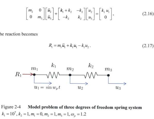
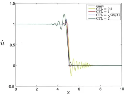
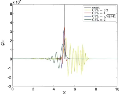
3.2.1. 1-D bar impact

Considering the impact of an elastic bar on a rigid wall problem (Fig. 3-5) where the governing wave equation is

2_{u = - aU}

(3.24)

5x2 c 2 at2

where the wave speed co is 5000, the 1-D 2-node elements of size Ax = 0.05 are used to