Clustering-based method for the feeder selection to improve the characteristics of load shedding

HAL Id: hal-02268669

https://hal.archives-ouvertes.fr/hal-02268669v2

Submitted on 6 Oct 2019

HAL is a multi-disciplinary open access

archive for the deposit and dissemination of

sci-entific research documents, whether they are

pub-lished or not. The documents may come from

teaching and research institutions in France or

abroad, or from public or private research centers.

L’archive ouverte pluridisciplinaire HAL, est

destinée au dépôt et à la diffusion de documents

scientifiques de niveau recherche, publiés ou non,

émanant des établissements d’enseignement et de

recherche français ou étrangers, des laboratoires

publics ou privés.

Clustering-based method for the feeder selection to

improve the characteristics of load shedding

Barnabé Potel, Florent Cadoux, Leticia de Alvaro Garcia, Vincent

Debusschere

To cite this version:

Barnabé Potel, Florent Cadoux, Leticia de Alvaro Garcia, Vincent Debusschere. Clustering-based

method for the feeder selection to improve the characteristics of load shedding. IET Smart Grid,

Institution of Engineering and Technology, In press, �10.1049/iet-stg.2019.0064�. �hal-02268669v2�

IET Smart Grid

Research Article

Clustering-based method for the feeder

selection to improve the characteristics of

load shedding

Barnabé Potel

, Florent Cadoux

_{, Leticia De Alvaro Garcia}

_{, Vincent Debusschere}

1_{University of Grenoble Alpes, CNRS, Grenoble INP, G2Elab, 38000 Grenoble, France} 2_{Enedis, Paris, France}

E-mail: [email protected]

Abstract: Under-frequency load shedding (UFLS) schemes are designed by specifying a given amount of load to shed at

various frequency thresholds to prevent the collapse of the electrical power system in the event of a large generation-load imbalance. An UFLS step is constituted of a group of medium-voltage feeders that trip when a given frequency threshold is reached. This study focuses on the method to be used when allocating a given feeder to a given step. First, the authors introduce performance metrics to quantify the accuracy level with which the UFLS target is met. Second, they model: the allocation method currently used in France; a variant of that method; and a new method introduced in this study, based on an automated clustering technique. Third, based on real consumption patterns measured from a vast area in France, and using the introduced performance metrics, they compare the efficiency of the three described methods. This study is conducted for the current state of loading of the considered distribution network and for a hypothetical situation with an increased share of distribution-side photovoltaic generation. For the chosen performance metrics, they demonstrate that the first two methods provide similar results while the clustering-based method performs remarkably better.

1 Introduction

Large power imbalances may lead to the blackout of the electrical power system (EPS). Those imbalances are directly reflected by the frequency of the power system, which decreases when consumption is higher than generation [1], and conversely. As a last resort to avoid a black-out when load exceeds generation, under-frequency relays are thus usually implemented by power system operators. In France, these relays are located at the head of medium-voltage (MV) feeders, inside primary substations, and they are set to trigger whenever a given frequency threshold is reached [2]. When this occurs, some parts of the distribution system are thus disconnected from the transmission system, reducing the total load, and containing the frequency decrease. This mechanism is called the under-frequency load shedding (UFLS) scheme.

It is of extreme importance to carefully design the UFLS scheme and to ensure in particular that the amount of load that will be shed is appropriate: indeed, not shedding enough load would not contain the frequency drop and thus not prevent the occurrence of a blackout, while shedding too much load would be counterproductive. Ideally, the amount of load shed should counterbalance as accurately as possible the power imbalance that causes the frequency drop, thus ‘freezing’ the value of frequency.

In practice however, this ideal seems out of reach; indeed, during a large power system event, the response of the UFLS must be very fast, and the situation is often complex (e.g. cascading failures or disconnection of high-voltage lines may lead to a situation where the power system is split into various parts, each of these sub-systems suffering from its own internal imbalance).

Therefore, conventional UFLS schemes are traditionally designed in a simpler and more robust manner, by specifying a

given amount of load to disconnect at predefined frequency thresholds. More precisely, the target amount of load to shed is commonly defined as a percentage of the total consumption of the

national network. The total load that will be shed at a particular

frequency threshold is called ‘step’ of the UFLS scheme. The number of steps and the amount of load which is shed [3–5] directly impacts the performances of the UFLS [6, 7].

As an example, the UFLS scheme in France, provided in Table 1, is currently composed of four steps, each one representing ∼20% of the total consumption of the distribution system. Each of these steps contains a list of thousands of feeders. Accordingly, four frequency thresholds are defined, respectively, at 49, 48.5, 48 and 47.5 Hz. The last 20% of the load is reserved for priority feeders composed of critical loads such as hospitals, government facilities and so on. This group of feeders should never be shed [8] and thus does not constitute an UFLS step, properly speaking. In addition, MV feeders that host only generators, but no loads, do not take part into the UFLS scheme.

In practice today, in France, the list of the feeders that constitute a particular UFLS step is updated once a year. We will retain this assumption in the present paper, as it does not seem practical on the short term to significantly shorten this reallocation period. Indeed, many of the UFLS relays that are deployed in the field today rely on technologies that require manual work, on premises inside the primary substation, whenever the frequency threshold is to be changed. We considered that this manual work cannot realistically be carried out more than once a year.

1.1 Current trends and literature review

The legacy UFLS schemes that have been deployed so far in various countries, in particular in Europe, are expected to evolve in the coming years for several reasons. The first reason is regulatory evolution, as currently seen in European network codes, and the second is the increasing share of distributed generation (DG) integrated in the power system.

1.1.1 Regulatory evolution: With the aim of improving the

harmonisation and reliability of the European power system, the European transmission system operators association, ENTSO-E,

Table 1 Current French UFLS scheme (% of the

distribution system load) [8]

Step 1 2 3 4

frequency, Hz 49 48.5 48 47.5

shed load, % 20 20 20 20

maintains a set of network codes that defines a common framework across European countries for the operation of the EPS. In particular, the UFLS mechanism (also known as ‘low-frequency demand disconnection’) is partially specified in the Network Code on Emergency and Restoration (NC-ER) [9] which was adopted on 24 November 2017 and which entered into force on 18 December 2017. The NC-ER compels ENTSO-E members to fulfil a number of specific requirements such as the number of steps, the range within which the amount of load to shed at each step should lie, the frequency interval between two steps and the range of the total load to shed. The notion of ‘range within which the amount of load to shed at each step should lie’ will be of particular importance in the present paper. Indeed, the ratio between the active power consumption of any group of feeders on the one hand, and the total national load on the other hand, is not perfectly constant; in practice, this ratio evolves over time, and as a consequence the weight of a given UFLS step is never perfectly equal to the target value. Those variations may have a critical impact on the efficiency of the UFLS scheme [10]. This problem occurred during the black-out event in Italy, 2003 [11]: [...] The plan is ‘hard wired’ and

tuned at peak load periods and it is therefore impossible to hourly adapt the load to guarantee the same percentage ready to be shed at any given time. [...] and during the 2015 black-out in Turkey

[12]: [...] The slightly different percentages of load shedding

reached on the March 31st result are due to a system loading difference to the reference load. [...]. These excerpts demonstrate

that it is crucial, both for regulatory compliance and for practical efficiency of the UFLS scheme, to consider the fact that the relative weight of pre-defined UFLS steps will unavoidably vary over time.

1.1.2 Impact of the DG: In addition, the number and total

capacity of generators that are tied to the distribution network is increasing steadily in France and many other countries, under the effect of massive distributed renewable energy sources (DRES) deployment. This trend is challenging the traditional UFLS scheme

[13–15]; indeed, the consumption profile of many feeders now results both from local consumption and from local generation – not from local loads alone any more. This potentially increases the risk that the weight of a particular UFLS step will vary wildly over time and drift away from its target weight. This phenomenon is studied in [13], where the authors use data from the main French distribution system operator (DSO) to determine impacts of photovoltaic (PV) penetration on different methods of feeder ranking.

Therefore, the UFLS scheme will probably become more adaptive in the future. It requires enhanced relay technologies allowing frequent updates of the frequency threshold assigned to each relay. They may also use additional ‘richer’ measurements such as rate of change of frequency [16–18], the second-derivative of frequency [19], a forecast of the frequency evolution [20, 21] and/or voltage measurements [22, 23]. Indeed, improving the adequacy between the amount of load shed on one hand, and the initial power imbalance on the other hand, may require:

• Additional measurements, to better estimate the appropriate UFLS action to apply at any given time (ex ante), and also to find out the appropriate reaction to a given power imbalance in near real-time when it occurs (ex post);

• A control infrastructure, including a communication system, that will apply and automatically update some new ‘dynamic’ UFLS scheme;

• A proper distribution of UFLS relays into the transmission system in order to take into account the entire load of the EPS. By comparison with this futuristic view on the topic of UFLS technology, recall that our assumption in the remainder of this paper is that the parameters of existing UFLS relays may currently not realistically be updated more than about once a year. In addition, the proposed study is limited to the analysis of various load curves of MV feeders. This means that only the active power is studied to check the load that could be shed if the UFLS is activated. The impact on voltage is not studied for several reasons: • It would be necessary to simulate both the distribution system

(because it is MV feeders that are shed) and the transmission system (because the UFLS deals with the active power imbalance) to study the impact of the load shedding on the voltage. Such simulations are difficult to implement, because of the quantity of data needed: it would require to know the various parameters of the lines, the generators and the loads and their variations in the time.

• The voltage conditions of the power system vary at each moment. The selection/allocation of feeders is done only once a year. In this case, it is not possible to monitor the possible ‘future’ impact on the voltage when the selected feeders may be triggered.

• Feeder allocation is region-wide. Thus, allocated feeders are geographically distributed over the national grid – this condition is also a requirement of the NC-ER. Thus, when load shedding

occurs, the impact on the voltage should also be distributed geographically.

1.2 Contributions and organisation of the present paper

In this paper, we first introduce in Section 3 some performance metrics that make it possible to meaningfully compare the efficiency of various UFLS schemes. We then discuss three methods (the method currently being used in France, and two new ones) for constituting the UFLS steps in Section 4. In Section 5, we compare these three methods by means of simulations and according to our proposed performance metrics; we also assess how our results are impacted by the growing share of photovoltaic generation. Finally, in Section 6, we summarise our work and provide some practical recommendations based on our simulations results.

Note that all simulations are conducted on real data measured over 2 years – first year for training and second for testing – from a vast area in France (roughly 1/25th of the territory) at the primary substation level of the main DSO, Enedis.

2 UFLS principles and challenges

2.1 Current scheme

In the French power system, as most of the other power systems (Fig. 1), large-scale generation capacity is connected to the transmission system. Some large loads such as energy-intensive industries are also directly connected to the transmission system, Fig. 1  Power systems, sub-systems and load shedding

e.g. railways networks, metalworking industries and so on. On the contrary, most DRES are connected to the distribution system, either to MV or low-voltage (LV) feeders. Such generators may be connected either to the same feeders as loads (so-called ‘mixed feeders’) or to specific ones (so-called ‘dedicated feeders’).

In France, non-priority MV feeders are re-allocated once a year to one of the four steps of the UFLS scheme. The re-allocation currently obeys the following protocol: the consumption of each MV feeder on the third Thursday of January at 9 am is recorded, and this measurement defines the weight of the considered MV feeder. Then four steps of (nearly) equal ‘weight’ are constructed manually by the operators, leaving aside the priority feeders.

An important characteristic of the current French UFLS scheme (presented in Table 1) is that it specifies the weight of each step

with respect to the distribution system load only (e.g. ‘the total

active power load of all the feeders allocated to step 1 should be roughly equal to 20% of the total active power consumption of the entire national distribution system load’). On the contrary, the NC

-ER specifies the weight of UFLS steps in terms of the total

national load. This makes a substantial difference, because a

significant amount of load is connected directly to the transmission system. Concretely, the actual weight of each step of the current French UFLS scheme, as a fraction of the total national load, is actually well below 20%.

During the event of 2006 [24], for instance, it was estimated a posteriori that the first UFLS step of the French scheme contained about 15% of the national load at the time of the event. Since, in addition, only about 80% of the relays of the first step actually triggered, the amount of load that was shed weighted about 12% of the national load [25]. The fact that the first UFLS step contained about 15% of the national load is quite representative; indeed, it is commonly accepted that the French distribution network represents roughly ∼75% of the national consumption. More accurately, the share of the national consumption served through the distribution networks varied between 65 and 80% over the year 2015 [26, 27].

2.2 NC-ER requirements

The NC-ER requires to replace the traditional French UFLS scheme with a new one composed of more steps, each one shedding a smaller amount of load. This should theoretically present a more ‘linear’ response to the frequency decrease, and distribute load shedding more evenly across various European countries.

In order to fulfil the NC-ER requirements, continental European countries have to respect those specifics terms [9]:

• There must be at least six steps;

• All steps shall shed a minimum of 5% of the national load; • All steps shall shed a maximum of 10% of the national load; • The total load shed should be 45% of the national load with a

margin of _{±7%, that is to say within the interval 38–52%.} One NC-ER-compliant scheme is proposed in Table 2. In this table, contrary to Table 1, the percentage values are defined with respect to the national load.

To comply with the NC-ER requirements, the total load involved in the UFLS scheme must remain between 38 and 52% of the national load at every instant. In France, this represents around 60% of the distribution system load, significantly less than in the current scheme (Table 1) where up to 80% of the distribution system load may be shed. This gives the DSO additional freedom in the choice of the feeders that will take part into the UFLS scheme. From the DSO point of view, the main question is then: what feeders should be allocated in order to have the best

compliance with the NC-ER? This is the question we tackle in the present paper.

3 Performance indicators for the comparison of

UFLS schemes

3.1 Target load to shed at regional level

Another important consideration is the geographical area over which the UFLS target is specified. As the implementation of UFLS is a responsibility of transmission system operators (TSOs), it seems natural to consider that the relevant geographical area is either the footprint of each TSO, or the national network (that is to say, the global footprint of all the TSOs inside a given country). In France however, UFLS steps are constituted at the regional level, independently from one region to the other. This is motivated first by the fact that local operators know their local network well, and second by the will to obtain a geographically even distribution of load shedding over the EPS. As a consequence, although the UFLS objectives are nation-wide, the implementation of the UFLS plan is actually local.

This raises the following issue: what should be the objectives of each of the ‘local UFLS scheme’? Said otherwise, how should the national UFLS objectives be scaled down and shared among individual regions? This scaling to a region is done by considering the following ratio: ‘energy consumed by the region during the last year’ divided by ‘energy consumed by the national system over the same period’

Robjt= α ⋅ βR⋅ nt (1)

where α is the ratio to shed, here 45% for the cumulative allocated

consumption and 7.5% for each step, as defined in Table 2, βR is

the ratio of the mean consumption of the region R at year (y − 1) over the mean consumption of the distribution network at year (y − 1), nt is the consumption of national network at the instant t.

This method ensures that summing all the objectives of all the regions of the distribution system will indeed yield the national objective to shed – at least for the training data.

3.2 What are good performance indicators?

A comparison of various methods needs efficiency criteria. Here, the objective is not to design new UFLS schemes but to identify an efficient method to characterise the compliance of the allocation with a given UFLS scheme. Thus, the allocated consumption for each step, and the sum over all steps, are compared to the target defined in the considered UFLS scheme. The analysed scheme is the one defined in Table 2, which is compliant with the NC-ER.

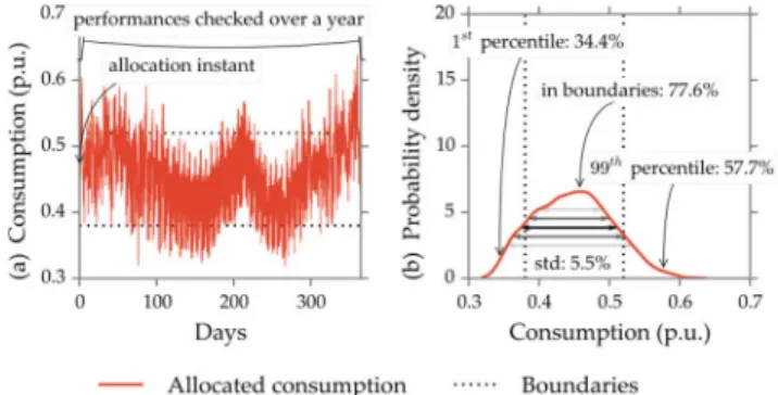
The following indicators, shown in Fig. 2, are proposed to evaluate the performances of an allocation regarding the total allocated consumption:

• The 1st and 99th percentiles provide information on the maximum deviations to the objective. As we are using field data, some may have extreme variations. Thus, it is better not to use the minimum and maximum values which may be distorted. • The standard deviation provides the dispersion of the allocated

consumption. This indicator is not dependent of one-time and large variations, contrary to the percentiles.

• The ratio/percentage within boundaries is the fraction of time when the NC-ER is respected.

In this paper, the allocated consumption is defined as the ratio of the consumption of the allocated feeders over the consumption of

Table 2 NC-ER compliant UFLS scheme

Step 1 2 3 4 5 6

frequency, Hz 49 48.8 48.6 48.4 48.2 48

shed load, % 7.5 7.5 7.5 7.5 7.5 7.5

the national system scaled at the considered level (as in (1) with

α = 1).

The proposed indicators are subject to the following shortcomings: the network topology, voltage regulation – which has an impact on load consumption – and power flows – especially to determine overloads risks – are not taken into account. Only the power consumption of feeders, distribution system and national system are studied. On the other hand, the above-mentioned indicators have the merit of simplicity. The more complex phenomena that are not captured by these indicators must thus be handled manually by the operators, as they are today in practice; for instance, for some primary substations where large generators are connected (typically on dedicated feeders) while load is modest, the operators may decide to not allocate the load-feeding feeders to any UFLS step, in order to avoid potential local over-voltage problems (with potential cascading effects) just after triggering an UFLS step.

3.3 Fraction of time spent within the NC-ER bounds

This criterion represents the fraction of time for which the NC-ER

requirements are satisfied over a one-year period. It is defined mathematically as the integral of the probability density function of the consumption ratio of allocated feeders between the NC-ER

bounds, as defined in the following equation: ratio in NC‐ER boundaries =

∫

binf

bsup

h(c)dc, (2)

where h is the density probability of the allocated consumption defined in p.u. over the considered year (Fig. 2b), b_inf, b_sup are the boundaries in which the allocated consumption has to remain to satisfy the NC-ER requirements. Here, 0.38 and 0.52 p.u.

(45% ± 7%) for the total consumption, and for each step, 0.05 and 0.1 p.u. (_{7.5% ± 2.5%).}

4 Allocation methods

In this study, three methods are compared:

(i) Traditional: The allocated consumption is computed based on a one-time measurement of the feeders consumption. This is done once a year. It is the method currently implemented in France. (ii) Mean: The allocated consumption is computed based on the mean consumption of the feeders.

(iii) Clustering: The allocated consumption is computed with a clustering-based allocation method.

The allocation period for the three methods is chosen to be one year. It could be possible to reduce this allocation period, nevertheless, the training data – used to calculate the mean consumption or compute the clustering – should be representative of the load pattern. For instance, for an allocation period of one day, the training data could be the consumption of the previous day; but for an allocation period of 6 months, the training data should be the same 6 months of the previous year (in order to account for seasonal variations); and so on. These considerations are left outside of the scope of this paper, due to our initial assumption that updating the settings of the UFLS relays more than once a year is not practically feasible today.

4.1 Current method – traditional

The method currently used in France defines the weight of a feeder as its consumption at a specific day and hour (reference date), namely on the third Thursday of January at 9 am in the current implementation of the method. Afterwards, feeders taking part into the UFLS scheme are chosen so that the total weight matches the target percentage of load to be shed.

More precisely, feeders are first ordered according to their k-factor defined below, and then selected one by one in this order until the target weight is reached. This allows the operators to

choose one particular allocation among the huge set of allocations that match the target weight. The k-factor is defined as

K =_{LV customers + MV customers}MV customers + 1 (3) The purpose of the K coefficient is to limit the impact of the UFLS scheme on industrial consumers, which are mainly connected at the MV level.

This method is easy to implement: the operators only need taking into account a one-time measurement; the calculations to perform are simple; and the method determines the allocation for the whole year to come. Again, this method is currently applied in France at the regional scale.

The outcome of this method obviously depends on the choice of the reference date: Fig. 3 shows the impact of this choice on the fraction of time during which the NC-ER requirements are

satisfied.

Various reference dates are tested over the month of January 2016. A weekly pattern clearly stands out; from this figure, it appears that weekends and night times should not be picked as the reference date for the traditional allocation method. The best choices are the working days during daytime (8 am to 6 pm). The current choice of the main French DSO Enedis, which is to select the third Thursday of January at 9 am, thus appears to be relevant. With this choice, the fraction of time spent within the NC-ER

bounds nearly reaches 80%.

4.2 Mean method

With this method, the weight of a feeder is defined as its average consumption during the previous year. Then feeders may be allocated just as for the traditional method, selecting them one by one in increasing order of their K coefficient, until the sum of the weights reaches the target. The rationale behind this method is that it does not depend on the choice of any particular reference date, so that it is somewhat less arbitrary than the traditional method, and should thus eventually perform better overall. Our simulation results below will demonstrate that this expectation may not actually be fulfilled.

What we call here the ‘mean method’ is essentially the same as the method proposed in [28], which was recommended by a Fig. 2  Example of indicators for a given allocation

Fig. 3  Parametric study: how much does the choice of the reference date

previous version of the Operation Handbook [29] – except for one additional subtlety related to so-called ‘back-feeding periods’. These periods are defined the times of the year during which the considered MV feeder is a net generator and feeds back active power into the primary substation. What the Handbook states about these back-feeding periods is that, when their total duration over a year is expected to exceed a given duration, the TSO has to decide whether the feeder should be taken into account for the UFLS allocation or not. In this study, we simply take into consideration the feeders whose mean demand over the year is positive, and ignore the others (they are never allocated).

The mean method thus only differs from the traditional method in two respects: first, the definition of the weight of a feeder if different; and second, some feeders may be discarded beforehand when using the mean method, whenever the yearly average consumption of these feeders is negative.

4.3 Clustering-based method

In this section, we introduce a new method for choosing the MV feeders which take part into the UFLS scheme. We term it the ‘clustering method’.

4.3.1 Motivations and rationale: A first important idea behind

the clustering method is that the notion of ‘weight’ of a feeder, whichever definition of ‘weight’ is chosen, is reductive and even crude: better allocation results could be expected if the entire profile (i.e. time series) of each feeder was taken into account.

A second consideration, which mitigates the first, is that we obviously have to choose the UFLS allocation before it is used hence, before the actual profile of each feeder is revealed. This means that we will have to rely, not on the actual time series (which is unknown future data), but on some kind of forecast based on past data. The point here is that these forecasts will probably not be very accurate at the level of individual feeders; whereas the sum (or the average) of forecasts for a large group of feeders should be much better, thanks to independent forecasting errors cancelling out. As a consequence, we argue that the allocation method should preferably rely on the characteristics of groups of feeders (‘clusters’, in our terminology) rather than on the characteristics of individual feeders (which would raise the risk of overfitting the forecasted data).

A third important idea behind the clustering method is that it dismisses the notion of ‘K coefficient’ entirely: we argue that, of (i) Minimising the impact of load shedding on MV customers. (ii) Maximising the fraction of time during which the weight of a certain group of feeders, selected for participation in the UFLS scheme, does lie within some prescribed bounds.

The second requirement should take precedence. As a consequence, the clustering method selects feeders according solely to their ability to produce UFLS steps with nearly constant weight, regardless of the number of MV and LV customers that are connected to any particular feeder.

Now, what method could we use to select a subset of feeders with a desired mathematical property – here, having a nearly constant weight with respect to the national load? Since any large power system will comprise thousands to tens of thousands of feeders, considering all possible subsets leads to combinatorial explosion and is thus highly impractical.

The notion of clustering aims at solving this problem, as follows: we will first group feeders into so-called ‘clusters’ of feeders with similar characteristics; and then consider the problem of choosing the feeders which take part into the UFLS scheme as a blending problem, where fractions of each cluster must be sampled and then blended together to produce the desired output. As the number of clusters is smaller than the original number of feeders, and most importantly, because the blending problem is continuous (not discrete), this formulation does not lead to combinatorial explosion; it is numerically tractable. The next section explains this idea in more detail.

This clustering-based method is composed of three steps: first the clustering itself, then the optimisation (i.e. solving the blending problem), and finally the selection of the individual feeders. Each of these three is detailed below.

4.3.2 Clustering step: This step consists in grouping the feeders

in clusters of feeders with similar load profiles.

We first observe that two feeders with similar profiles but different scaling factors (e.g. one being approximately twice the other) should be considered similar for our purpose, but would actually be considered very different by any clustering algorithm. To solve this issue, we start by pre-processing the data as follows: we divide each profile (time series) by its mean value. Due to this scaling step, the yearly average consumption of any scaled profile is equal to 1, and two feeders with similar profiles but initially different scaling factors will now look similar indeed to a clustering algorithm.

Then the scaled profiles are fed into a clustering algorithm, whose aim is to group them based on the similarity of their scaled consumption pattern. For this purpose, we use the standard K-means method, whose main idea is to build NC clusters (NC being a

user-defined constant) in such a way that their total within-cluster variance is minimised min

∑

∑

∑

where NT is the time set, NC is the number of clusters, f is the

feeder consumption, Ci is the cluster i, μCi is the consumption of

the cluster i.

There are several variants and implementations of the K-means method. We used the K-means++ [30] algorithm, which is straightforward to understand, easy to implement and fast to compute – which are important attributes when dealing with large datasets such as ours. Our method is however general and does not depend on the specific choice of the means method and the K-means++ implementation of this method: any other clustering algorithm could have been used.

The K-means method depends on two main user-defined parameters: first the number of clusters NC, and second the

initialisation of the algorithm. The K-means algorithm usually performs well compared to other clustering techniques [31] provided that the number of clusters [32] is large enough for the considered dataset. According to our experiments discussed in Section 4.3.5 (see also [33]), setting this parameter to NC:= 20

appears to be a good choice for our application. The impact of the initialisation of the algorithm is discussed in Section 5.5 and is shown to have a limited impact on the results.

As a result of the clustering phase, the feeders are categorised into NC= 20 groups with similar scaled profiles. Each cluster is

characterised by its members (i.e. the individual feeders that belong to the considered cluster) and by its mean profile; the mean profile of a cluster may be interpreted as a prototypical profile that was not present in the input data but to which all the members of a cluster are similar.

These clusters, each with their mean profile, are the input data of the subsequent optimisation step.

4.3.3 Optimisation: This step is based on the idea that the UFLS

scheme may be conveniently created by taking x% of the mean

profile of the first cluster, y% of the mean profile of the second

cluster and so on. Said otherwise, creating the UFLS scheme amounts to solving a blending problem. In practice, this may be achieved by solving the following mathematical formulation:

min

∑

∑

where Robjt is the load to shed for region R as defined in (1), αi is

the allocated ratio of the cluster i, μCit is the relative consumption

of the cluster i for the sample t.

In plain words, we simply optimise a least-squares performance metric under the constraint that the blend should contain no less than 0 and no more than 100% of each cluster. This problem may be solved directly using any off-the-shelf algorithm for bounds-constrained optimisation [34].

Again, our method does not depend on the specifics of the least-square formulation (5): any other type of regression – such as quantile regression [35] – could have been used. Such more elaborate methods may yield better results; however, in this article we aimed at simplicity and thus contented ourselves with the simple least-square formulation (5).

After applying the optimisation step, we end up with the numerical value of the coefficients αi, said otherwise, with a

blending formula that tells us how to create the desired UFLS scheme: by sampling α1% of the first cluster, α2% of the second cluster and so on, and then blending all these samples together. The next section explains how this sampling and blending step is performed.

4.3.4 Sampling feeders from clusters: Given the list of

members, the mean profile and the blending coefficient αi of the

considered ith cluster, the sampling step is performed as follows: • We iterate over the members of the considered cluster (in any

particular order);

• We try adding the current iterate to the UFLS scheme that we are constituting;

• If this addition makes the profile of the UFLS scheme closer than before (in the least-squares sense) to the target (which is αi

times the mean profile of the cluster as in (5)), then the addition is validated and the current iterate is added to the UFLS scheme; • Otherwise the addition is cancelled, the current iterate is removed from the UFLS scheme and the next iterate is processed.

After this step, we end up with the desired output: our UFLS scheme has been created by specifying which feeder is allocated or not. The creation of the steps from these allocated feeders is discussed in Section 5.2.1.

4.3.5 Illustration of the clustering method: In order to

complement the above theoretical description of the clustering method with more concrete examples, this section provides some illustrative results. We also discuss the choice of parameter NC, the

user-defined number of clusters. The data is composed of the historical load curves of 1274 feeders over 2 years, with a time step of half an hour (see Section 5).

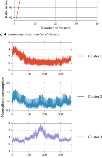
Let us first consider the influence of parameter NC. Fig. 4

shows one of the performance indicators – ratio within the boundaries – depending on the chosen number of clusters. Note that this simple study uses a non-causal allocation method, in the sense that the data used to perform the allocation (training dataset) is the same as the data used to compute the performance metric (simulation dataset).

If there is only one cluster, the clustering-based method is similar to the mean-method (without using the K-factor). A knee point appears at about four clusters, as in a similar study on a distribution system loads [36]. A higher number of clusters allows to reach better performances (99.2% for 40 clusters in the boundaries versus 91.8% for one cluster). Thus, for a non-causal

computation, the number of clusters should be chosen as high as

possible. However, this no longer holds when the causality requirement is taken into account. After extensive causal numerical experiments, we fixed the number of clusters to NC= 20.

Let us now consider in more detail the kind of results that come out of the clustering step. To illustrate this step, an example of the mean profile (i.e. averaged scaled consumption) of three different clusters is shown in Fig. 5. This figure provides a typical example

of the kind of variations that may be encountered among the various clusters. These load curves correspond to the net

consumption of the feeders which includes loads and DG – as

photovoltaic generation in residential areas.

• The first cluster is, at the beginning of the year, consuming active power. However, starting from April, the consumption may become negative: this cluster thus represents mixed feeders, perhaps hosting a significant amount of PV generators – this would explain why the net demand is particularly low during the summer season.

• The second cluster is consuming power all around the year, and exhibits a clear weekly pattern while the yearly pattern is only moderate.

• The third cluster is composed of feeders which exhibit a strong yearly pattern, with an increased consumption during the summer season.

Let us now provide an example of the results of the optimisation step and of the sampling step.

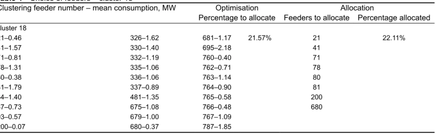
Table 3 shows an example of ratios coming from the optimisation and Table 4 provides an example of the feeders’ choice done from the feeders in the cluster #18 for the given optimisation. In this particular instance, cluster #18 was constituted of 30 feeders (the first being feeder #21 and the last, feeder #787). At the optimisation stage, it was found that 21.57% of this cluster Fig. 4  Parametric study: number of clusters

should ideally participate to the UFLS. After selecting eight feeders (the first being feed #21 and the last, feeder #680) from the short-list of 30, the actual weight of the selected feeders was 22.11% of the total weight of the cluster, reasonably close to the target value of 21.57%. This is quite typical: we observed that there are usually enough feeders in a cluster to obtain, after the allocation step, a good approximation of the target weight that came out of the optimisation step.

It is worth noting that in practice, the results of the optimisation very often lead to selecting some clusters entirely, and to ignoring some others entirely: the so-called ‘percentage to allocate’ that comes out of the optimisation phase is often equal to 0 or 100% – as depicted in Table 3. Only for a few clusters does the ratio lie strictly between these boundaries. Indeed, the consumption profile of some clusters is quite similar to the national consumption profile, and such clusters tend to be favoured by the optimisation – as the error to the objective is thus minimal for them.

As a consequence, the sampling phase is meaningful only for a minority of the clusters, and is trivial for the others – those clusters for which either all of none of the cluster members are selected. This is why we did not refine the sampling procedure, and did not try in particular to define a preference order (such as using the K-factor just as for the traditional allocation method currently used in France, or avoiding to allocate mixed feeders in order to avoid disconnecting distributed generators) in the sampling phase: this would have made little difference on the results anyway.

For the whole process (clustering, optimisation, feeders’ choice and step creation), the computation time is below 10 min. The longest part is the pre-processing, i.e. retrieve the data from the feeders (1274 here, more than 20,000 for the whole French distribution network) and convert it in the appropriate format.

5 Application to a French region

The proposed study is based on data provided by the major French DSO, Enedis, which represents the load curves in 2015 and 2016 of 1274 MV feeders with a time step of half an hour. The nation-wide and distribution-grid-wide load curves were retrieved from [26, 27]. Using this data, we realised the allocation using the three methods defined previously. Then, the results are compared using the performance indicators defined in Section 3 while considering the NC-ER requirements (presented in Section 2.2). The results are

analysed, first considering the total allocated consumption, then considering the different steps of load shedding.

The objectives are used as defined in Section 2.2: to shed totally 45% of the national consumption scaled to our region and 7.5% for each step. The total allocated consumption and the step consumption should be, respectively, in the boundaries [0.38 p.u., 0.52 p.u.] and [0.05 p.u., 0.1 p.u.].

• The traditional method is conducted using the consumption of the _{21 January 2016 at 9 am of the feeders. The feeders are} allocated using an increasing factor K until the total weight fits the objective at the time of allocation.

• The mean method is conducted using the average consumption of the feeders from the _{21 January 2015 to the 21 January 2016.} The feeders are allocated using an increasing factor K until the total weight fits the mean consumption of the objective. • The clustering method is conducted using the consumption of

the feeders from the 21 January 2015 to the 21 January 2016. The optimisation is realised with these clusters to fit the corresponding objective. The feeders are allocated according to the optimised ratios of the clusters.

5.1 Total allocated consumption

We apply the three above-mentioned methods on our dataset and first consider the total load allocated for the UFLS, regardless of individual UFLS steps. The corresponding probability density function is depicted in Fig. 6. The boundaries of the NC-ER are also indicated.

The traditional and mean methods provide very similar, and relatively disappointing, results: a very significant fraction of time is spent outside of the NC-ER boundaries. On the contrary, the clustering-based method is performing much better: the consumption allocated to UFLS almost always lies within the boundaries.

Table 3 Optimisation realised on clusters – ratio to allocate

Cluster no. 1 2 3 4 5 6 7 8 9 10

ratio to allocate, % 66.18 0 100 100 52.14 100 100 42.58 100 0

cluster no. 11 12 13 14 15 16 17 18 19 20

ratio to allocate, % 100 37.68 91.86 0 100 0 100 21.57 100 100

Table 4 Choice of feeders – cluster 18

Clustering feeder number – mean consumption, MW Optimisation Allocation

Percentage to allocate Feeders to allocate Percentage allocated

cluster 18 21–0.46 326–1.62 681–1.17 21.57% 21 22.11% 41–1.57 330–1.40 695–2.18 41 71–0.81 332–1.19 760–0.40 71 78–1.31 335–1.06 762–0.71 78 80–0.38 336–1.06 763–1.14 80 81–1.79 337–0.89 764–0.90 81 84–1.40 481–1.35 765–0.58 200 87–0.73 675–1.08 766–0.48 680 93–0.57 679–1.00 767–1.09 200–0.07 680–0.37 787–1.85

5.2 Individual steps

5.2.1 Creation of the steps: The steps are created in a second

phase. Once the feeders are chosen to be allocated, they are divided into the required number of steps. This can be done using various methods. We propose the use of the same methods defined previously.

s1, s2…sS are the objective ratios to shed for each step.

For the clustering method, feeders can be divided into each step with the following process:

(1) Realise a clustering over all allocated feeders.

(2) Choose a ratio of s1/(s1+ s2+ ⋯ + sS) in each cluster to create

the first step, take the feeders out.

(3) Choose a ratio of s2/(s2+ ⋯ + sS) in each cluster to create the

second step, take the feeders out. (4) …

(5) For the last step, take all remaining feeders.

For the traditional and mean methods, feeders can be divided into each step with the following process:

(1) Arrange all feeders by their increasing coefficients K.

(2) Take first feeders whose the sum of the weights (consumption at allocation instant or mean consumption) is close to objective to shed, to create the first step.

(3) Take next feeders whose the sum of the weights is close to objective to shed, to create the second step.

(4) …

(5) For the last step, take all remaining feeders.

5.2.2 Results: Fig. 7 shows the allocated consumption of the six

steps for the traditional, the mean and the clustering methods. Each step is almost contained within the boundaries defined by the NC-ER. The steps obtained with the traditional and mean methods are quite similar.

The steps obtained with the clustering method have the same probability density shape and the same standard deviation. Step 5 is a bit over-filled while steps 6, 3 and 2 are a bit under-filled. This difference comes from two reasons:

(i) Sampling an exact fraction from a given cluster is not always possible (this is a drawback of the clustering method);

(ii) The consumption data for 2015 and 2016 is different (this is a drawback of the causality requirement).

5.3 Summary of results

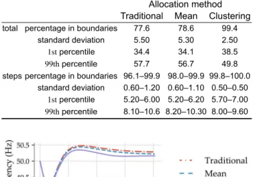
Table 5 gives the values of all the proposed indicators, defined in Section 3, for the allocated consumption of 2016 for the three methods.

The constraint on the steps is less stringent than the constraint on the total allocated consumption: the percentage within boundaries are close to 100% for all methods for the steps while this percentage is around 78% for the traditional – which is coherent with Fig. 3 and the chosen date of 21 January at 9 am – and mean methods for the total allocated consumption. The steps are composed of less feeders than the total allocation, which should lead to higher variations of their consumption. Nevertheless, their ‘relative’ boundaries are less stringent in the end:

• For the individual steps, the relative boundaries are ( ± 2.5%)/7.5% = ± 33.3%;

• For the total allocated consumption, the relative boundaries are ( ± 7%)/45% = ± 15.6%.

The variations for the steps may thus be twice as large than the variations for the total allocated consumption, relatively speaking. As a consequence, it is easier to satisfy the NC-ER requirements

for the individual steps than globally for the entire set of allocated feeders. The quality of an allocation method should thus be judged essentially based on its ability to satisfy the global constraint imposed by the NC-ER, not based on the individual step constraints

which are less stringent and easier to fulfil.

We thus now focus on the global constraint: to satisfy it, recall that the first and the last percentiles shall be higher than 38% and lower than 52%, respectively. The traditional and the mean methods are equally distributed over these two percentiles: the first is around 34% (−4 to 38%) and the last around 57% (+5 to 52%). The clustering method performs much better according to this criterion: the fraction of time spent within boundaries is close to 100% and the standard deviation is divided by two compared to the other methods.

5.4 Impact on frequency evolution

Fig. 8 shows the frequency evolution of the three methods for an initial unbalance of 5%. The load shed per method corresponds to the 99th percentile of the step of Table 5: 10.6% for the traditional method, 10.3% for the mean method and 9.6% for the clustering method. The 99th percentile of the step is chosen in order to highlight that, the larger the variations of the allocated Fig. 7  Probability densities of the consumption steps

Table 5 Indicators for the three methods (%) – year 2016

Allocation method Traditional Mean Clustering

total percentage in boundaries 77.6 78.6 99.4

standard deviation 5.50 5.30 2.50

1st percentile 34.4 34.1 38.5

99th percentile 57.7 56.7 49.8

steps percentage in boundaries 96.1–99.9 98.0–99.9 99.8–100.0 standard deviation 0.60–1.20 0.60–1.10 0.50–0.50

1st percentile 5.20–6.00 5.20–6.20 5.70–7.00 99th percentile 8.10–10.6 8.20–10.30 8.00–9.60

consumption, the more affected the frequency response. Thus, as the variations of the allocated consumption are different for the three methods, the frequency evolution also is. The model used is the one developed in [7], based on the one used by ENTSO-E [5].

At the beginning, the frequency is decreasing according to the unbalance and the inertia of the system (swing equation). When it reaches 49 Hz, the three methods are shedding different amounts of load. The traditional method is shedding a greater amount than the mean method and the mean method a greater amount of the clustering method. Thus, the frequency for the traditional and mean method reaches higher values than that for the clustering method.

Table 6 shows the maximum and final values of the frequency for the realised simulation.

The slight difference in the load which is shed per method has a significant impact on the frequency value. The difference between the traditional and clustering method is 130 mHz for the maximum values and 110 mHz for the final values. As it is essential to avoid over-frequency situations when the UFLS is triggered, it is necessary to limit the variations of the weights of the steps and to respect as much as possible the objectives of the UFLS scheme.

5.5 Sensitivity to PV insertion

In order to determine the efficiency of UFLS when DRES, especially PV, is inserted in a substantial way into the distribution network, we simulate a change in the PV penetration rate. The choice of taking only PV is motivated by the fact that it is the most frequent type of DG encountered within mixed feeders. Indeed, the capacity of most wind turbines is so large that this type of generation technology is usually connected to the distribution network directly at primary substation level, through a dedicated MV feeder that will not participate in the UFLS.

Scenarios are made considering that PV is implemented evenly across feeders, including critical and dedicated ones. The objective to shed is thus updated, considering the same proportion of PV addition but scaled to the distribution network.

Fig. 9 shows the evolution of the indicators for increasing values of peak PV production until 1 GWpeak for the considered region which has a mean consumption of 1.3 GW. The _{1 GWpeak} represents 1.2 GW installed (power load of 82.2% [37]).

The coloured area represent the spread of the methods: for the mean and traditional ones, there is no spread; while the clustering method has a spread due to the algorithm used to create the clusters with K-means++ [30]. This algorithm has a randomly chosen initialisation point. Fifteen simulations have been conducted for each increase to highlight the impact of the initialisation.

A degradation of all indicators is observed for all three methods when PV is added. For the traditional method, respect of the NC

-ER is decreasing linearly from 78 to 65%. The 99th percentile remains close to 60% while the 1st one is evolving from 34 till 25%. As before, the mean method is quite similar to the traditional one. The clustering method however provides better robustness with respect to PV insertion: indicators are evolving with a lower sensitivity than for the two other methods. Although the standard deviation is increasing, the respect remains over 95% for the overall range and the 1st and 99th percentiles remain close to the boundaries. For the three methods, the increase of the standard deviation is significant for the first step of PV production increase (100 MW). It is due to the used shape of the PV production: this production has been retrieved at the national level and may have differences with the local production in the considered region.

6 Conclusion and recommendations

This paper proposes to improve the feeder selection method for load shedding by using a new method based on clustering, and compares it with two previously existing methods. The comparison is made regarding the ability of the allocated feeders to disconnect the specified amount of load at any time over the whole year, as the allocation is realised manually just once a year, in order to respect the NC-ER. To perform such a comparison, several indicators are defined: 1st and 99th percentiles, standard deviation and time ratio of NC-ER respect.

The traditional and mean methods have similar performances according to the proposed indicators, while the clustering method shows improved performances. The latter uses the data of the year

y − 1 to determine which feeders should be allocated for the year y

by considering their entire consumption profiles over the year. With this method, the standard deviation of the allocated consumption is halved compared to the two other ones. In particular, the time ratio of NC-ER respect is nearly 100% for the clustering method, while the traditional method and the one recommended by ENTSO-E do not meet this requirement. Thus, we advise TSOs and DSOs to favour the implementation of a more sophisticated method, such as the clustering-based method, for the feeder selection. Moreover, instead of defining only boundaries within which the allocated consumption has to be at all time, requirements should also define a time ratio for the respect of these boundaries to give more degree of freedom for the implementation; indeed, the current requirements of the NC-ER seem overly stringent and might be simply impossible to fulfil.

A sensitivity study of the allocation methods about the insertion of PV in the distribution network highlights the robustness of the clustering method, whose indicators are significantly less impacted than the ones of the other two methods. Nevertheless, a high penetration of DRES may conduct to high variations of the allocated consumption. This should be taken into account for the set-up of new standards and grid codes.

7 Acknowledgments

The work reported in the paper has been developed in the framework of the Enedis Industrial Research Chair on Smart Grids.

8 References

[1] Kundur, P., Balu, N.J., Lauby, M.G.: ‘Power system stability and control’ (McGraw-hill, New York, 1994), Vol. 7

[2] Delfino, B., Massucco, S., Morini, A., et al.: ‘Implementation and comparison of different under frequency load-shedding schemes’. 2001 Power

Table 6 Frequency maximum and final values for the three

methods

Allocation method

Frequency Traditional Mean Clustering

maximum, Hz 50.48 50.44 50.35

final, Hz 50.27 50.21 50.16

Engineering Society Summer Meeting. Conf. Proc. (Cat. No.01CH37262), Vancouver, BC, Canada, 2001, Vol. 1, pp. 307–312

[3] Bogovic, J., Rudez, U., Mihalic, R.: ‘Probability-based approach for parametrisation of traditional underfrequency load-shedding schemes’, IET Gener. Transm. Distrib., 2015, 9, (16), pp. 2625–2632

[4] Ceja-Gomez, F., Qadri, S.S., Galiana, F.D.: ‘Under-frequency load shedding via integer programming’, IEEE Trans. Power Syst., 2012, 27, (3), pp. 1387– 1394

[5] ENTSO-E: ‘Technical background for the low frequency demand disconnection requirements’, Nov. 2014

[6] Santos, A.Q., Monaro, R.M., Coury, D.V., et al.: ‘New scoring metric for load shedding in multi-control area systems’, IET Gener. Transm. Distrib., 2017,

11, (5), pp. 1179–1186

[7] Potel, B., Debusschere, V., Cadoux, F., et al.: ‘Under-frequency load shedding schemes characteristics and performance criteria’. 2017 IEEE Manchester PowerTech, Manchester, 2017, pp. 1–6

[8] Arrêté du 5 juillet 1990 fixant les consignes générales de délestages sur les réseaux électriques [Ministerial Decree of the 5th July 1990 setting the general rules of load shedding of electrical power systems]

[9] ENTSO-E: ‘Network code on emergency and restoration’

[10] Sigrist, L., Rouco, L.: ‘Design of UFLS schemes taking into account load variation’. 2014 Power Systems Computation Conf., Wroclaw, 2014, pp. 1–7 [11] UCTE: ‘FINAL REPORT of the investigation committee on the 28 September

2003 blackout in Italy’

[12] ENTSO-E: ‘Report on blackout in Turkey on 31st march 2015’

[13] De Boeck, S., Van Hertem, D.: ‘Integration of distributed PV in existing and future UFLS schemes’, IEEE Trans. Smart Grid, 2018, 9, (2), pp. 876–885 [14] Das, K., Nitsas, A., Altin, M., et al.: ‘Improved load-shedding scheme

considering distributed generation’, IEEE Trans. Power Deliv., 2017, 32, (1), pp. 515–524

[15] Albrecht, M., Robitzky, L., Rehtanz, C.: ‘Selective and decentralized underfrequency protection schemes in the distribution grid’. 2017 IEEE Manchester PowerTech, Manchester, 2017, pp. 1–6

[16] Terzija, V.V.: ‘Adaptive underfrequency load shedding based on the magnitude of the disturbance estimation’, IEEE Trans. Power Syst., 2006, 21, (3), pp. 1260–1266

[17] Seyedi, H., Sanaye-Pasand, M.: ‘New centralised adaptive load-shedding algorithms to mitigate power system blackouts’, IET Gener. Transm. Distrib., 2009, 3, (1), pp. 99–114

[18] Rudez, U., Mihalic, R.: ‘Monitoring the first frequency derivative to improve adaptive underfrequency load-shedding schemes’, IEEE Trans. Power Syst., 2011, 26, (2), pp. 839–846

[19] Jallad, J., Mekhilef, S., Mokhlis, H., et al.: ‘Improved UFLS with consideration of power deficit during shedding process and flexible load selection’, IET Renew. Power Gener., 2018, 12, (5), pp. 565–575

[20] Rudez, U., Mihalic, R.: ‘WAMS-Based underfrequency load shedding with short-term frequency prediction’, IEEE Trans. Power Deliv., 2016, 31, (4), pp. 1912–1920

[21] Potel, B., Debusschere, V., Cadoux, F., et al.: ‘A real-time adjustment method of conventional under-frequency load shedding thresholds’, IEEE Trans. Power Deliv., 2019, DOI: 10.1109/TPWRD.2019.2900594

[22] Hoseinzadeh, B., Faria da Silva, F.M., Bak, C.L.: ‘Adaptive tuning of frequency thresholds using voltage drop data in decentralized load shedding’, IEEE Trans. Power Syst., 2015, 30, (4), pp. 2055–2062

[23] Saffarian, A., Sanaye-Pasand, M.: ‘Enhancement of power system stability using adaptive combinational load shedding methods’, IEEE Trans. Power Syst., 2011, 26, (3), pp. 1010–1020

[24] System Disturbance on 4 November 2006, Final Report, UCTE, Feb. 2007 [25] Commission de régulation de l’énergie (2007). Rapport d'enquête de la

commission de régulation de l’énergie sur la panne d’électricité du samedi 4 novembre 2006 [Report of the electrical blackout of the 4th November, 2006] [26] Open Data Réseaux Énergies (ODRÉ) Available at

https://opendata.reseaux-energies.fr/ [Accessed Aug. 7, 2019]

[27] Open Data Enedis Available at https://www.enedis.fr/open-data [Accessed Aug. 7, 2019]

[28] VDE. Technische Anforderungen an die automatische Frequenzentlastung [Technical requirements for automated load shedding], Jun. 2012

[29] ENTSO-E. Continental Europe Operation Handbook. RG CE OH- Policy 5: Emergency Operations V 3.1. Sep. 2017

[30] Arthur, D., Vassilvitskii, S.: ‘k-means++: the advantages of careful seeding’. Proc. of the eighteenth annual ACM-SIAM symp. on Discrete algorithms. Society for Industrial and Applied Mathematics, New Orleans, USA, January 2007, pp. 1027–1035

[31] Tsekouras, G.J., Hatziargyriou, N.D., Dialynas, E.N.: ‘Two-stage pattern recognition of load curves for classification of electricity customers’, IEEE Trans. Power Syst., 2007, 22, (3), pp. 1120–1128

[32] Chicco, G.: ‘Overview and performance assessment of the clustering methods for electrical load pattern grouping’, Energy, 2012, 42, (1), pp. 68–80 [33] Chicco, G., Napoli, R., Piglione, F.: ‘Comparisons among clustering

techniques for electricity customer classification’, IEEE Trans. Power Syst., 2006, 21, (2), pp. 933–940

[34] Byrd, R. H., Lu, P., Nocedal, J., et al.: ‘A limited memory algorithm for bound constrained optimization’, SIAM J. Sci. Comput., 1995, 16, (5), pp. 1190–1208

[35] Koenker, R., Bassett Jr, G.: ‘Regression quantiles’, Econ.: J. Econ. Soc., 1978, 46, pp. 33–50

[36] Mutanen, A., Ruska, M., Repo, S., et al.: ‘Customer classification and load profiling method for distribution systems’, IEEE Trans. Power Deliv., 2011,

26, (3), pp. 1755–1763

[37] RTE Bilan électrique 2015. Available at https://www.rte-france.com/fr/article/ bilans-electriques-nationaux [Accessed Aug. 7, 2019]