A cost efficient maintenance inventory policy for the Massachusetts Bay Transportation Authority

A Cost Efficient Maintenance Inventory Policy for the

Massachusetts Bay Transportation Authority

By

Ryan Wren McWhorter B.S., Physics (1996)

Baylor University Sc.M, Physics (1997)

Brown University

Submitted to the Department of Civil and Environmental Engineering In Partial Fulfillment of the Requirements for the Degree of

Master of Engineering in Logistics At the

Massachusetts Institute of Technology June 1999

© 1999 Massachusetts Institute of Technology

All Rights Reserved

Signature of Author...

Department

Certified by...

...

of Civil and Environmental Engineering May 7, 1999

-.... ..

James M. Masters Executive Director, Master of Engineerig in Logistics Program Thesis Supervisor

A ccepted by ... . ... AndrVT-Fhittle Chairman, Department Committee on Graduate Students

A Cost Efficient Maintenance Inventory Policy for the

Massachusetts Bay Transportation Authority

By

Ryan Wren M'Whorter

Submitted to the Department of Civil and Environmental Engineering On May 7, 1999 in Partial Fulfillment of the

Requirements for the Degree of Master of Engineering in Logistics

ABSTRACT

This thesis examines the role of optimal maintenance inventory and supply chain practices in public transportation planning by focusing on the Massachusetts Bay

Transportation Authority (MBTA).

Maintenance and procurement planning play a critical, yet research-neglected role in transit operations. Private sector companies have reduced spending while improving service levels by conducting research into inventory planning and implementing their conclusions. The strategies used in the private sector can be applied to meet the same objectives in public transit.

Literature of performance measures and mathematical formulae is reviewed. A one-for-one replenishment system for repairable items is analyzed under the framework of a transit agency, and a variety of ordering policies are compared. The effect of sub-depots on the amount of required inventory parts is examined. The current inventory practices of the MBTA are detailed along with areas of improvement and future areas of research.

Thesis Supervisor: James M. Masters

Title: Executive Director, Master of Engineering in Logistics Program Massachusetts Institute of Technology

Acknowledgements

This work would not have been possible without the help of many people. I give considerable thanks to Jim Masters for allowing me to study the application of logistics and supply chain management to my interests in public transportation. His guidance, resources, and humor made the thesis project memorable and enjoyable. I would also like to thank the many people of the Massachusetts Bay Transportation Authority who offered tours of their facilities, numerous stories, and T memorabilia. Dave McGrath gratefully offered his time for me to visit and ask questions to gather my information. Finally, Cindy's effort to reference, review and help rewrite my entire thesis was a tremendous help. Her encouragement and understanding helped make the MIT experience attainable and rewarding.

Table of Contents Page A bstract ... 2 Table of Contents ... 4 List of Figures ... 6 List of Tables...7 List of A ppendices... 7 1 IN TRODU CTION ... 8

1.1 Public Transportation O verview ... 8

1.2 Procurem ent and M aintenance ... 10

1.3 Capital Spares Buys... 12

1.4 Supply Chain M anagem ent ... 12

1.5 Structure of Thesis... 13

2 LITERATU RE REVIEW ... 14

2.1 M aintenance Function ... 14

2.2 Perform ance M easures ... 15

2.3 Capital Expenditures ... 18

2.3.1 Mathematical Background-Expectation Values... 19

2.3.2 Palm 's Theorem Justification... 20

2.3.3 Proof of Palm 's Theorem ... 22

2.3.4 Expected Backorders... 25

2.3.5 A vailability... 29

Table of Contents (Continued)

Page

2.3.7 M ulti-Indenture Theory... 34

2.3.8 VARIM ETRIC ... 37

2.3.9 Applications of VARIMETRIC ... 42

2.3.10 Comparison of Inventory Policies... 43

2.3.11 M ulti-Echelon Extension... 44

2.4 Supply Chain M anagement ... 45

3 MASSACHUSETTS BAY TRANSPORTATION AUTHORITY ... 48

3 .1 B u d get ... 4 8 3.2 M aterials M anagement Department ... 50

3.3 M BTA Performance Measures...51

4 RESULTS AND CONCLUSIONS... 54

4.1 Areas of Improvement at the MBTA ... 54

4.2 Capital Expenses ... 55

4.3 Inventory M anagement... 55

List of Figures

Page

1.1-1 Public Transportation Ridership... 10

1.1-2 Federal Transit Funding ... 11

2.1-1 The Articles of Quality M anagement... 15

2.2-1 Performance Measures of Efficiency and Effectiveness... 16

2.3.4-1 Optimal Function of EBO vs. Cost ... 28

2.3.5-1 System Availability ... 30

2.3.8-1 Base-Depot Demand... 39

2.3.11-1 Sub-Depot System Design... 45

3.1-1 FY 1998 Budget ... 48

3.1-2 Time Series of Capital Expenditures... 49

3.3-1 Time Series of Cost Efficiency ... 52

3.3-2 Revenue Vehicle M iles Time Series ... 52

4.3-1 Inventory Reorder Points and Safety Stock ... 56

List of Tables

Page

1.1-1 Em ission Com parison ... 9

2.3.4-1 Stock Level Expected Backorders... 26

2.3.4-2 M arginal Cost Analysis... 27

2.3.4-3 Inventory Purchases ... 28

2.3.6-1 Inventory Storage M atrix ... 33

2.3.7-1 LRU Fam ily Tree ... 35

3.3-1 MBTA vs. SEPTA Performance Measures... 53

4.3-1 Partner Contingencies... 57 List of Appendices Page A M ETRIC Calculations... 62 B M OD -M ETRIC ... 63 C VARIM ETRIC ... 65

Chapter 1 INTRODUCTION

Within the last decade, the federal government has observed the positive effects of increased public transportation and has allocated the largest funding to date toward mass transit systems. Maintenance and procurement planning play a critical, yet research-neglected role in transit operations. Private sector companies have reduced spending while improving service levels by conducting research into inventory planning and implementing their conclusions. This paper will investigate the application of optimal maintenance inventory and supply chain practices toward public transportation planning by focusing on the Massachusetts Bay Transportation Authority (MBTA).

1.1 Public Transportation Overview

Increased use of public transportation can reduce energy consumption, relieve traffic congestion, and decrease the rising levels of air pollution. Studies by the

American Public Transit Association (APTA) (Transit Fact Book, 1998) have shown that a 10% increase in nationwide public transit ridership could save 135 million gallons of gasoline, and a 10% increase in ridership in only the five largest cities could save 85 million gallons of gasoline annually. Their studies also show that a heavy rail subway train six cars long and filled with passengers would be equivalent to a line of cars the

length of 95 city blocks. Concerning the environment, a small number of commuters switching to mass transit can have a large effect on hazardous emissions. APTA studies reveal that a single-person automobile will produce 200 times the hydrocarbon emissions and over 700 times the carbon monoxide emissions of electrified rail, see Table 1.1-1.

Mode Hydrocarbons Carbon Monoxide

(grams/passengr-mile) (grams/passenger-mile)

Electric Rail 0.01 0.02

Singe-Person Auto 2.09 15.06

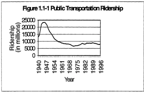
Despite these benefits, ridership levels and government funding of mass transit declined from the 1940's through the 1980's (Haven, 1980; Transit Fact Book, 1998). Following World War II, fuel rationing ceased, and America was enjoying an economic boom. Gasoline prices dropped, and the government favored policies that initiated low-density suburban growth. Furthering a decline in public transit ridership, President Eisenhower signed the Defense Interstate Highway Act in 1956 allowing states to invest in large highways with 90% government funding. Figure 1.1-1 shows the effects of these changes on public transit ridership with usage dropping to an all-time low of 6 billion passengers in 1972. This represents a drop of 72% from the 1945 rate of over 23 billion passengers per year (Transit Fact Book, 1998).

Recent political opinion has reversed this trend by noting the positive effects that transit can have on energy consumption, traffic congestion and air pollution. In 1991, the federal government passed the Intermodal Surface Transportation Efficiency Act, ISTEA,

allowing federal money normally used to aid highway construction only, to be spent on either highway or transit projects. Also, in 1993, the Omnibus Budget Reconciliation Act

allowed a $0.02 portion of the highway trust fund tax per motor vehicle to be placed in a mass transit account.

Emission Comparison Table 1.1-1

Both of these acts, and the extension of the ISTEA program through the year 2001, show the federal government's willingness to focus on public transportation and its benefits. These efforts have resulted in more money being spent in the public transportation sector. Figure 1.1-2 shows dollar figures allocated to transportation by the federal government. Budget projections for the year 2000 predict that an allotment totaling $6 billion will be reserved for public transportation funding (Transit Fact Book, 1998).

1.2 Procurement and Maintenance

With increased spending in public transportation, efficient use of resources is necessary to ensure higher service levels that will support growing ridership estimates. One department of mass transit organizations with a focus on service quality is the maintenance and procurement division. The ultimate role of a maintenance and

procurement manager is to provide an increased service level. Constraining this goal is

Figie 1.1-1 Rtic Transportaion

adership

25000

.2- 0 2MX

E10000

Ec.

5000

0

I

Year

Figte

1.1-2 Federal Transit Rundng

the secondary objective of maintaining adequate inventory levels such that costs are minimized. Maintenance can carry up to one-fifth of the cost of operations (Robbins and Galway, 1995), and procurement can spend in excess of $200 million on rolling stock alone (National Transit Database, 1999). In spite of the large fraction of a transportation budget disbursed in maintenance and procurement, limited research has focused on the utilization of inventory planning as a source of cost-reduction for a transit organization. In fact, two transit journal reports focusing on innovative maintenance programs do not mention spares planning except to note their absence in current literature (Robbins and Galway, 1998; Inventory Management for Bus and Rail Public Transit Systems, 1995).

In the private sector, many manufacturing companies have focused on inventories as a source of cost reduction opportunities. Although a transit agency operates in a different environment, the goal is the same: maintenance managers want to maximize spares availability while minimizing inventory investment. This paper will focus on the application of logistics and supply chain management in two areas of the maintenance

function for transit organizations, purchasing high-cost repairable items and the reduction of the procurement lead time.

1.3 Capital Spares Buys

An optimized ordering plan for purchasing spare maintenance parts in a one-for-one replenishment system was developed by Feeney and Sherbrooke (1966), followed by Sherbrooke (1968). METRIC, their product, is an algorithm that determines the optimal number and type of items to buy and where to house them in a multi-echelon structure. Muckstadt (1973) further developed this work by including part families, or

multi-indenture items, in what he titled MODMETRIC. Slay (1984) considered the variance of the demand mean in a multi-echelon, multi-indenture structure in an inventory ordering

algorithm entitled VARIMETRIC. Muckstadt and Thomas (1980) analyzed various inventory plans and found that an item decomposition method, such as METRIC, performs better than level decomposition and a "days of supply" system. Sherbrooke

(1986) studied the three item decomposition techniques and found VARIMETRIC to be

the most accurate. Work by Malec and Steinhorn (1980) shows the effects of

infrastructure on both the service level and the necessary number of maintenance spares.

1.4 Supply Chain Management

Supply chain management covers many areas. This paper will focus on applying supply chain techniques that decrease procurement lead times and safety stock for consumable spare parts inventory. In the private sector, this is a well-studied problem. Most notable is the work of Kurt Salmon Associates in the apparel industry. Quick

Response, a program created by Kurt Salmon Associates and used by the apparel industry to reduce clothing lead times from 25 weeks to 2 weeks, can increase a retailer's return on assets and sales by 7-12% and 20-40%, respectively (Hammond and Kelly, 1990). The transit management environment, however, is far different from a fashion retail organization. Where fashion designs can change over long lead times, most

consumables, such as an oil filter, will always be in demand. For a transit organization, long lead times increase both the amount of stored inventory, safety stock and the probability of a stock-out. Byrnes and Shapiro (1991) analyzed the value of

intercompany operating ties and the benefits of partner relations and information sharing on safety stock and inventory levels.

1.5 Structure of Thesis

Chapter 2 will review the literature of current maintenance innovations, performance measures, and the different inventory ordering policies, including METRIC,

MODMETRIC, and VARIMETRIC. Chapter 2 will also review the effect of sub-depots on the number of inventory parts and the resulting cost vs. benefit of adding

infrastructure. Chapter 3 will detail inventory practices and performance measures of the Massachusetts Bay Transportation Authority (MBTA). Chapter 4 will present the results and conclusions of a new inventory planning policy for the MBTA along with areas of future research. Details of all calculations will be given in the appendices.

Chapter 2 LITERATURE REVIEW

2.1 Maintenance Function

The goal of a maintenance department is to "apply resources in a cost-effective manner to help meet the service objectives of the agency: on-time delivery of clean, comfortable, and reliable [vehicles] (Robbins and Galway, 1995)." Note the similarity to the logistics goals of manufacturing and distribution companies who try to "meet

customer demands at a competitive cost while maximizing customer value through adaptability to a continuous change environment (Klaus, 1999)." The strategies used in the private sector can be applied to meet the same objectives in public transit.

Cost-efficiencies are achieved through the effective use of capital, labor and information, see Figure 2.1-1. These three aspects can alter the quality of a maintenance program. In a steady-state budget, sacrifices must be made between these areas without a resulting reduction in service quality (Fielding, 1987). For instance, improved inventory management can reduce the required number of spare parts and more efficiently make purchases, which translates into improved capital spending. Improved information can facilitate the evaluation of current practices by highlighting areas of restriction or

progress, thus data flow could be used for performance measurement and planning. Also, information, such as technological or innovational discoveries, can be shared across transit agencies. Maintenance labor can be optimized by studying the difference in a transit agency that hires generalist or specialist workers in a given area, or if some jobs

should be in-house or contracted to other companies or agencies. This paper will focus on one of these areas of the maintenance function, the capital expenditures.

Figure 2.1-1 The Articles of Quality Management

Capital

Labor

Information

2.2 Performance Measures

A common management philosophy is strategic planning. This theory combines

long and short term planning of budgetary information in a stochastic, complex

environment. To monitor a strategic plan, goals must be set and performance measures put in place to track the effectiveness of a plan. In the past, public transit agencies concentrated on ridership as the prominent measure of a successful operation. Now, performance measures focus not only on consumption, but also on service inputs and outputs (Fielding, 1987).

Fielding (1987) describes performance measures for public transit management based on principal concepts that are measurable. He considers service inputs, such as

and service consumption, such as passenger miles, operating revenue or total passengers. From these dimensions, relationships describing efficiency and effectiveness can be determined, see Figure 2.2-1. A cost effectiveness ratio measures the fraction of service inputs to service consumption, such as fuel expense per passenger mile, and illustrates how effectively the organization is using its resources in generating consumption. Service effectiveness ratios weigh the fraction of imparted to consumed service, such as capacity miles per passenger miles. A service effectiveness ratio measures the

organization's capability to efficiently meet its demands. Cost efficiencies illustrate the fraction of service input to service output, such as maintenance expense per revenue vehicle mile. These ratios describe the organization's ability to use its resources to produce service. This paper will focus on cost efficiency by attempting to decrease maintenance expense while increasing availability.

Figure 2.2-1 Performance Measures of Efficiency and Effectiveness

Service InpuE

Cost

0fNOI*VCyr

Service Consumption

In general, there are two classes of measures, the time-series analysis and the cross-sectional analysis. A time-series approach plots the performance of an entity across time. This method displays trends that an organization might be following or the effect

of new management and ideas. Since a change in system activity over the period of analysis can occur, a time-series measure should be followed by a summary of events during the given time period. A performance measure that shows a reduction in the ratio of passenger miles per revenue vehicle mile over a five-year period might not be isolated to a drop in ridership. The diminished ratio could be the product of an increase in

revenue vehicle miles with ridership not meeting the new capacity. These two depictions of the same performance measure result in different strategies and solutions.

A cross-sectional analysis compares common measures of peer groups. The

organizations in the peer group should have common characteristics. These organizations should be similar in size, perhaps by the number of peak vehicles, the peak to base ratio, or a similar operating speed. Houston Metro runs a large number of express commuter busses at highway speeds, while many of the Massachusetts Bay Transportation

Authority busses are operated as city routes running at a much lower average speed. Thus these two transit systems should not be in the same peer group where measures of vehicle speed are an issue. Another necessary criterion for peer groups is economic considerations. The median household income in New York City, NY in 1989 was

$38,445, much higher than the median household income of $26,151 in Birmingham, AL

(Median Household Income in 1989, 1999). This discrepancy could have a large effect on operating expenses and thus these agencies should not be in the same peer group.

2.3 Capital Expenditures

To ensure that vehicles remain operational following a malfunction, spares must be available for the replacement of broken components. Spare ratios describe the number of spare parts that are stored at a facility to ensure that during a disruption, a broken part can be instantly replaced. A high spare ratio corresponds to a large number of spares being stored for a given part. In determining the spare ratios for a maintenance facility, two aspects of inventory management must be addressed:

" Purchasing repairable capital spares inventories

e Managing consumable inventories

Each year, the federal government funds infrastructure improvements for transit agencies. These improvements are made to facilities, such as new buildings purchased or built, or to rolling stock like new rail cars or buses. When new trains are acquired, a number of expensive, repairable items are also ordered. Examples of typical capital spare items are train wheels, traction motors, and A/C units. The decision as to which items to purchase is made by recommendations from the train manufacturer along with input from experienced maintenance personnel. Characteristics taken into account are an item's expected failure rate, repair time, and unit cost (McGrath, 1999). These items, labeled capital spares, comprise a large fraction of the procurement budget (National Transit Database, 1999). The ability to procure capital spares in an optimal fashion can have a positive impact on vehicle availability. An effective ordering algorithm can lower spares ratios while keeping maintenance costs low and service levels high.

Managing the inventory of lower cost consumable items is equally important and requires a different algorithm than that for capital spares. Consumable parts are ordered

on a routine basis similar to a grocery store that orders and stocks its high utility

products. Examples of a consumable in a maintenance facility would be brake pads, oil filters, or halogen lamps. High utility consumables require usage monitoring and forecasting to accurately predict lead-time demands (McGrath, 1999). Carrying fast-moving consumables obligates the maintenance department to also hold sufficient safety

stock for covering unusual demand rates. An effective inventory management system can reduce on-hand inventory and increase availability.

2.3.1 Mathematical Background -Expectation Values

Probabilities are necessary in a model of inventory demand since part failures occur as a stochastic process (Sherbrooke, 1992). A complete picture of uncertain events can be attained through the use of expectation values. Expectation value equations weigh the probability of statistical outcomes whether they are costs, stock-outs, or backorders. The expectation value, also called the mean or average, is given mathematically as

E(x)= xPr(x) (2.3.1-1)

x=1

and the variance of the mean, also known as the standard deviation, is

Var(x) = E [x2]- (E[xD2 (2.3.1-2)

where

E[x2]= YX 2 Pr(x) (2.3.1-3)

2.3.2 Palm's Theorem Justification

Palm's theorem was first used to describe the number of telephone exchanges required at a telephone operator's switchboard. It has since been applied to fire

department planning, bus stop population, and stock requirements planning in the US Air Force.

For application of Palm's theorem, one must assume that given events follow a Poisson distribution, equation 2.3.2-1. An arrival process that is generated by a group of independent entities, each with a probability of generating an event in a given time interval, can be approximated by a Poisson distribution. This is an understandable

assumption for the arrival process of failed units, and empirical data shows that a Poisson process closely approximates real-world demand for spares within the boundaries of a long-run steady-state behavior and a lack of dependence among items that can cause contingent arrival densities (Crawford, 1981).

For subway maintenance operations, a long-run steady-state behavior can be appropriately justified. In special circumstances, this assumption is an implausible approximation. In the context of the US Air Force transitioning from peacetime to wartime activity, assuming a steady-state model is unreasonable and requires a different solution (Sherbrooke, 1992).

The Poisson distribution is described by the following equation where m is the average annual demand for repair of a given item, and T is the average repair time in years.

(mT)xe mT

Using the expectation value equation (2.3.1-1), the expectation or mean of the Poisson distribution is

E(x)= mT (2.3.2-2)

It is noted for future reference that the variance of the Poisson distribution is also mT. The inventory system studied in this thesis is the (S -1, S) replenishment system. The model represents expensive units that have lower repair costs than purchase costs, thus the term repairable item. The notation (S -1, S)refers to an initial inventory of S units where the reorder point, or in this case the repair point, corresponds to a drop in the inventory level to S -1. When the unit fails, it is immediately inventoried for repair. This is also known as a one-for-one replenishment system (Feeney and Sherbrooke,

1966).

The dilemma facing procurement managers is the choice in initial stock level S (Feeney and Sherbrooke, 1966). In transit service operations, a stock-out can result in a drop in service level. The maintenance manager is concerned with the intangible cost of a potential stock-out and the opportunity cost due to downtime. As these are usually incalculable costs, a failure to provide a necessary spare is oftentimes not given as a quantitative result. Another factor facing maintenance managers is the cost of providing an appreciably large number of stock units affording complete protection against stock-outs. The balance of these two costs, availability versus budget constraints, will be the principal factors in determining optimum stock levels for repairable items (Cho and Parlar, 1991).

The probability distribution of demands when stock level is zero is dependent upon the probability distribution of the number of units in repair. Therefore, to determine

the optimum stock level, the steady-state probability distribution of the number of units in repair, the inventory pipeline, must be known. Palm's theorem states that given a mean time to repair, regardless of its distribution, and the average demand, already assumed to be a Poisson random variable, the steady-state probability distribution of the number of units in repair will be Poisson with a known mean (Feeney and Sherbrooke, 1966).

Palm's Theorem - If demand for an item is a Poisson process with an annual

mean m, and if the repair time for each failed unit is independently and identically distributed according to any distribution with mean T years, then the steady-state probability distribution for the number of units in repair has a Poisson distribution with mean mT (Sherbrooke, 1992).

Therefore, Palm's theorem permits an estimation of the steady-state probability distribution of the number of units in repair from the mean of the repair time and demand rate. Given the importance to this paper that Palm's theorem provides as the foundation, a proof is necessary.

2.3.3 Proof of Palm's Theorem

This proof can be found in Hadley and Whitin (1963) and Sherbrooke (1992). The joint probability of n Poisson events occurring in the time interval t to t+dt is given

by

(e~""

using ti +t2 +.. .+tn = t, this can be rewritten as

Dividing equation 2.3.3-2 by the Poisson distribution for n events gives the conditional probability of n events.

mne-mtdt...

Therefore the probability that one event occurs between ti and dt; is (taking n=1),

d4

t (2.3.3-5)

Hence if one Poisson event has occurred in a given time interval, then the

probability for another occurrence during the time period t; +dt; is dt/t, independent of the

number of events that previously occurred. This will be an important derivation in understanding Palm's theorem.

Let h( ) represent the probability that a repair will be completed in time T The probability that an item entering the repair facility at time ti is completed at time t>t; is

t-t;

H(t -ti)= fh(TWd (2.3.3-6)

0

Using equation 2.3.3-5 the probability of a unit being repaired by time t, given that one

demand occurred between the time interval 0 to t, is

H(t-ti) _dtI

(2.3.3-7) t

!fH(T)T (2.3.3-8)

0

Using the binomial distribution, the probability describing the fraction of fulfilled demands can be known. Defining u as the maximum inventory, x as the inventory at time

t, and y as the demands up to time t, u-x is the number of units in repair and y+x-u would

be the number of completed repairs. Therefore the probability distribution for the u-x repairs of the y demands will be

bin(x)= (yu -4(1- t)J H(T)dT (1 / t)J l - H

(T)]dT

_ 0 _ , 0

Weighting this distribution by the Poisson probability of demands y gives

Pr[inventory = x

]=

Now let time t approach infinity.

F-mf(1-H (T))W t

Pr [inventory = x,]=

lim

f{1

This complicated formula can be simplified by noting that

im

{1-

in which case,

limPr(inventory

Thus the number of units in repair has a Poisson distribution of mean mT within the range

t = 0 to oo. Therefore, given a mean repair time and demand rate, Palm's theorem allows

2.3.4 Expected Backorders

The stock amount at any level of a warehouse system can be thought of as the sum of on-hand inventory and due-in stock minus the present backorders (Sherbrooke,

1992).

s = OH + DI-BO (2.3.4-1)

Consider an item that has a one-for-one replenishment policy where the standing stock level is one unit. If a failure occurs, the unit goes directly into repair. On-hand inventory drops to zero, and the number due in is raised to one with the stock level, s, remaining constant. If another failure occurs, the resulting stock-out initiates one

backorder, causing another unit to be ordered and due in. The stock level again remains constant throughout the system.

A maintenance manager is concerned with the expected number of backorders.

The goal, as stated before, is to minimize the expected backorders subject to a cost constraint. We can describe the number of backorders by the equation

As)=(X-S) if x>s (2.3.4-2)

=0 otherwise

where x is the number of failed units and s is the stock level. If the amount of inventory to be repaired is greater than the amount of stock on hand, backorders will occur.

Otherwise, when the failed units amount to less than the on-hand stock, there will be no backorders. Using the expectation value formula together with the number of backorders, the expected backorders can be given as

Note that when s = 0,

EBO(O)= xPr(x)= E(x)= mT (2.3.4-4)

x=1

If a decision must be made between two items in a single-depot model, marginal analysis can be used in conjunction with expected back orders to produce an optimal solution for procurement (Sherbrooke, 1992).

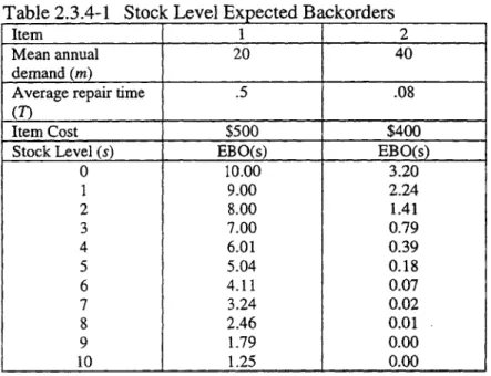
Consider two items that have independent average annual demands, average repair times and unit costs. Using equation 2.3.4-3 and 2.3.4-4 for expected backorders (EBO's), a table can be made listing EBO(s) for varying stock levels, see table 2.3.4-1.

Table 2.3.4-1 Stock Level Expected Backorders

To determine the optimum procurement policy, it is necessary to check the decrease in EBO(s) for differing stock purchases on the margin according the following equation EBO(s -1) - EBO(s) _(2.3.4-5) C Item 1 2 Mean annual 20 40 demand (m)

Average repair time .5 .08

(7) _ _ _ _ _

Item Cost $500 $400

Stock Level (s) EBO(s) EBO(s)

0 10.00 3.20 1 9.00 2.24 2 8.00 1.41 3 7.00 0.79 4 6.01 0.39 5 5.04 0.18 6 4.11 0.07 7 3.24 0.02 8 2.46 0.01 9 1.79 0.00 10 1.25 0.00

When no stock purchases are made, the total expected backorders is the sum of

Table 2.3.4-2 Marginal Cost Analysis

Item 1 Item 2

Stock (s) EBO(s) EBO(s -1) - EBO(s) EBO(s) EBO(s -1) - EBO(s)

0.5 0.4 0 10.00 - 3.20 -1 9.00 2.00 2.24 2.40 2 8.00 2.00 1.41 2.07 3 7.00 2.00 0.79 1.55 4 6.01 1.98 0.39 0.99 5 5.04 1.94 0.18 0.55 6 4.11 1.86 0.07 0.26 7 3.24 1.74 0.02 0.11 8 2.46 1.56 0.01 0.04 9 1.79 1.33 0.00 0.01 10 1.25 1.08 0.00 0.00

EBO(0) for item 1 and EBO(0) for item 2. The first purchase should correlate with the

unit that has the largest effect on expected backorders per unit cost. According to Table

2.3.3-2, the first purchase would be item 2 since its marginal EBO(1) = 2.40, while the

marginal EBO(1) = 2.00 for item 1. The next purchase would follow the same pattern:

Item 2 has a marginal EBO(2) = 2.07, while Item 1 has a marginal EBO (1) = 2.00, hence item 2 would be the next purchase. This algorithm is continued until a budget constraint or minimum EBO(s) desirability is reached. Table 2.3.4-3 shows the optimal purchasing plan for these items, and figure 2.3.4-1 illustrates the cost-backorder curve. The general form of the cost-backorder curve has a positive concavity extending to infinity.

Qualitatively, a small amount of investment can initially reduce the backorders by a large amount, but as the expected backorders tend to zero, the cost will increase at a

greater rate. Since transit organizations do not use expected backorders to relay information on performance, a connection with availability is useful.

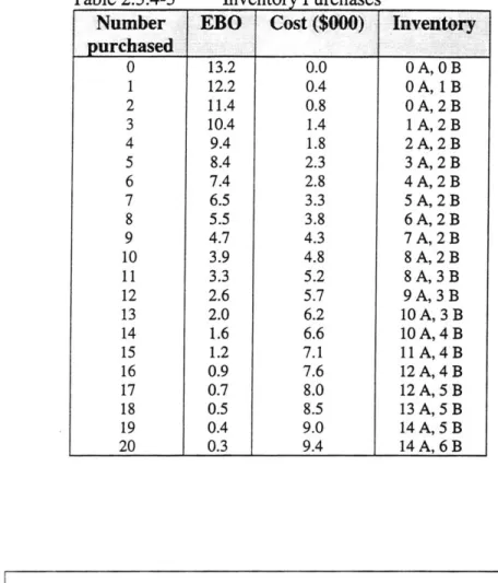
Table 2.3.4-3 Inventory Purchases

Number EBO Cost ($000) Inventory

purchased

Figure 2.3.4-1 Optimal fumction of EBO vs. cost

14.0 12.0 10.0 0 8.0 6.0 4.0 2.0 0.0 0 0.4 0.8 1.4 1.8 2.3 2.8 3.3 3.8 4.3 4.8 5.2 5.7 6.2 6.6 7.1 7.6 8.0 8.5 9.0 9.4 cost ($000)

2.3.5 Availability

Sherbrooke (1992) provides an excellent derivation of availability. In the context of a subway rail system, consider the sliding door motor found in train cabs.

Representing the door motor as part i on the train, let Zj be the number of i units on a train, and the number of trains be N. There would therefore be NZi locations of part i. For a system that has 40 cabs with 4 door motors per cab, the system would consist of

160 door motors. The probability of a door motor malfunctioning in the system equals

the total backorders for unit i divided by the total number of door motors in the system,

EBOi (Si) NZ,

The probability of availability is

1- (Si) _(2.3.5-2)

_NZi

The exponent corresponds to Zi occurrences of unit i. Overall availability for the entire system is a product over all parts, i = 1 to I. Therefore, a definition of availability for the train, given as a percentage, would be

EBQ (si

A=100J

NI]

A

EBQ(sj) '

=1

NZ

Taking the logarithm of both sides separates the different units.

A )EBO ( Si).

log =IZ, log 1- (2.3.5-5)

Expanding the logarithm using the approximation log(1 - x) = -x + -... (2.3.5-6) 2 gives A EBO (Si ) log Z, (2.3.5-7) 100 i=, NZ, log( -- -S E (2.3.5-8) 100 N

This last expression is a separable function of EBO's for the individual units. Since both a function and the logarithm of a function have their maximum at the same point in space, equation 2.3.5-8 proves that minimizing the expected backorders will

maximize the logarithm of availability, hence maximizing availability.

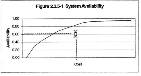
Figure 2.3.5-1 shows an ideal system availability curve. Given that much of the real world does not operate at optimality, a typical agency may procure parts such that their system lies within the optimum curve at point "X". By implementing an optimal ordering algorithm, an agency could either operate at the same cost with a better availability, or reduce costs and operate at the previous availability.

Figure 2.3.5-1 System Availability 1.00 0.80-S0.60 -- - - - -ccQ.40 0.20 0.00 Cost

2.3.6 METRIC

A common model used in maintenance operations is the multi-echelon inventory

system. This theory is characterized by large central depots and smaller local bases where inventory is held at more than one location. Feeney and Sherbrooke (1966)

developed an algorithm to determine what items to purchase and where to store them in a multi-echelon system. Here, the availability is maximized by the choice of item and location. The variables of METRIC theory are given below (Sherbrooke, 1992).

mj - average annual demand at base j

Tj - average repair time (in years) at base

j

pj - average annual pipeline at base j (mj * Tj)

rj - probability of repair at base j

Oj - average order-to-ship time from depot to base j

The subscript j refers to the bases, 1.. .J, and a zero subscript will designate depot information. The average annual demand on the depot will be a summation over all bases for those parts that cannot be repaired at their base,

m0 = m, (1- r)

(2.3.6-1)-The average depot pipeline is

po= MOTO (2.3.6-2)

If the depot does not have inventory on-hand, there will be an expected backorder

at the depot,

EBO(solm.To) (2.3.6-3)

The average pipeline for demand at base j will consist of the units repaired at the base,

miTir; (2.3.6-4)

plus a function of those that are not repaired at the base. For these items, the delay could be due to the average order-to-ship time,

(2.3.6-5) or a proportion of them could be backordered at the depot,

EBO(so moTo

)1

ld ein 0

The sum of these outcomes yields an equation for the average pipeline at base]j:

EBO(sojmaTo )

p= m, r +(1-

(iT

in

0O

(2.3.6-6)

(2.3.6-7)

As an example, consider a multi-echelon system of one depot and three identical bases. Let

mj= 35

Tj= .02 (in years) r= .25

Oj=.001

To= .02 (in years)

mo= 3*35*(1-.25) = 78.75

p = .02*78.75 = 1.575

The inventory pipeline at basej,

gj

tabulated using the EBO equation 2.3.6-3. Since base stock levels will be dependent on the depot stock level, expected backorder equations must be calculated for both depot and base stock levels of different size. A matrix must then be formed for all combinations of depot vs. base stock levels. Examples of the calculations are given in Appendix A.

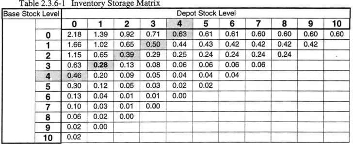
Table 2.3.6-1 shows one set of results. The shaded diagonal depicts the expected backorders for a variety of allocations of exactly four units of stock between the three bases and the depot. The minimum expected backorder for 4 units is .28, with 1 unit at the depot and 3 units designated for the bases. The exercise can be repeated if there are two or more items to purchase, in which case marginal analysis can determine optimality across items. Table 2.3.6-1 determines where to store the units, and marginal analysis, using an optimal expected backorders table similar to Table 2.3.4-3 for all units, selects among items.

Table 2.3.6-1 Inventory Storage Matrix

Base Stock Level Depot Stock Level

0 1 2 3 4 | 5 6 7 8 9 10 0 2.18 1.39 0.92 0.71 0.63 0.61 0.61 0.60 0.60 0.60 0.60 1 1.66 1.02 0.65 0.50 0.44 0.43 0.42 0.42 0.42 0.42 2 1.15 0.65 0.39 0.29 0.25 0.24 0.24 0.24 0.24 3 0.63 0.28 0.13 0.08 0.06 0.06 0.06 0.06 4 0.46 0.20 0.09 0.05 0.04 0.04 0.04 5 0.30 0.12 0.05 0.03 0.02 0.02 6 0.13 0.04 0.01 0.01 0.00 7 0.10 0.03 0.01 0.00 8 0.06 0.02 0.00 9

0.02 0.00

2.3.7 Multi-Indenture Theory

In the context of a subway rail system, consider the sliding door motor in a train cab. If the door motor malfunctions due to a loose air pressure valve, the entire motor should not be replaced, for only the replacement of the pressure valve is required. In this example, the door motor is labeled a Line-Replaceable Unit, or LRU, and the pressure valve is called a Shop-Replaceable Unit, or SRU. For repairable items, an LRU can be composed of many SRU's. This is multi-indenture inventory policy (Muckstadt, 1973). Following the same logic as METRIC, if the expectation values describing the number of LRU's in repair at a random point in time, also called the LRU pipeline, can be

determined, then the expected backorders for the LRU at the bases can be derived. Multi-indenture theory can be used in conjunction with multi-echelon theory, as Muckstadt (1973) shows. For clarity of exposition, a single echelon example will be introduced with multi-echelon, multi-indenture theory given in section 2.3.8 with an introduction to VARIMETRIC.

The number of LRU's in repair at a given point in time is the sum of the present LRU depot inventory pipeline plus those demands prior to repair time that were delayed due to an SRU stock-out. Consequently, the mean requires a sum over all SRU items

i...

.

E(xo)= m0TO + EBO(silmilT) (2.3.7-1)

where

mO = Xm (2.3.7-2)

The expected LRU base backorders can be calculated using the mean of the LRU depot pipeline, E(xo).

EBO(sejxo) (2.3.7-3)

This is the same logic applied in METRIC where the expected backorders, EBO(solxo),

were calculated by utilizing the mean of the pipeline, E(xo).

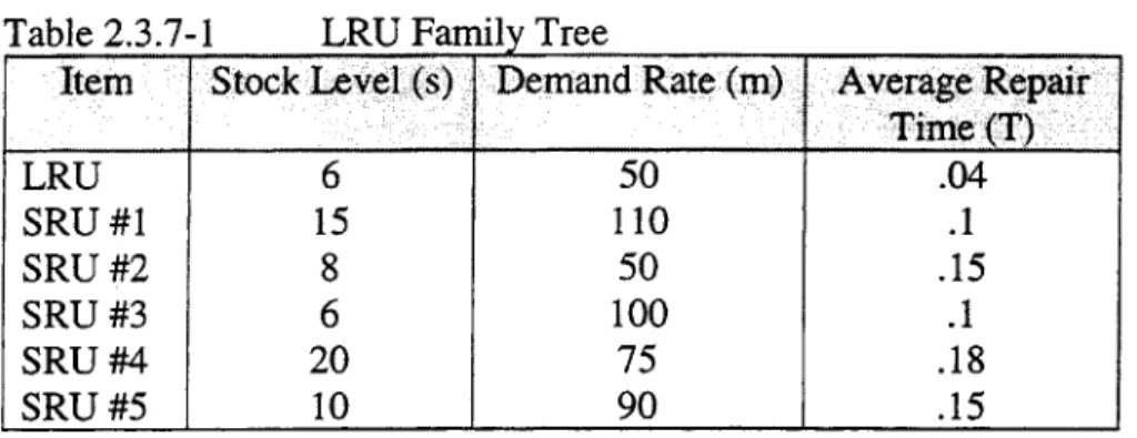
For modeling purposes, the required information consists of the stock levels, demand rates, and repair times for the LRU and its family of SRU's. Consider the information in Table 2.3.7-1

Table 2.3.7-1 LRU Family Tree

Item Stock Level (s) Demand Rate (m) Average Repair

Time (T) LRU 6 50 .04 SRU#1 15 110 .1 SRU#2 8 50 .15 SRU #3 6 100 .1 SRU #4 20 75 .18 SRU #5 10 90 .15 Using equation 2.3.7-1, E(xo)= 2+.216+.861+4.11+0.18+3.79 =11.05 (2.3.7-4). and EBO(6|11.05)= 5.11 (2.3.7-5)

Detailed calculations are given in Appendix B. Using this information, the same marginal cost analysis is followed as in Section 2.3.4 to determine the optimal ordering plan across LRU families. This model, called MODMETRIC, works well as a

preliminary approximation for EBO's, but it can underestimate expected backorders by as much as a factor of four (Sherbrooke, 1992).

The model's problem lies in the distribution assumed for the LRU depot pipeline.

It w c ta 4 te T PU hackorders had a pipeline that followed a Poisson

it was accepteU LIIL L1' ~ -- ~_

distribution. Recall from Section 2.3.2 that the variance of a Poisson distribution is equal to its mean. In practice, the variance of the pipeline is larger than the mean. In fact, for stock levels greater than zero, the variance-to-mean ratio of expected backorders will exceed one, and reach a maximum where the stock level equals the expectation value (Svoronos, 1986). Even though LRU and SRU demand is Poisson, the probability distribution for the LRU backorders is Poisson only when stock levels equals zero. Consequently, since an LRU is a composition of SRU backorder distributions, the LRU pipeline is Poisson only when the stock level for each SRU is equal to zero (Sherbrooke,

1992). Since the variance is a function of the stock level, a term in the expected

backorder equation should include the variance of the inventory pipeline.

For a multi-echelon system, the mean inventory pipeline for the number of LRU's in repair is (see equation 2.3.7-1),

E(xo

)=

Im;T

)

i=I

The variance of the pipeline can be derived from this equation since the variance of a sum is equal to the sum of the variances, and the number of units in depot repair is a Poisson process.

Var(xo)= moTo + VBO(sI|m;T1) (2.3.7-7)

Var(xo)= 2 +.693 + 2.39 + 8.88 + 0.26 +10.6 = 24.9 Giving a variance-to-mean ratio of

VTMR = 24. 1.05 = 2.24 (2.3.7-9)

Therefore, a distribution with a variance-to-mean ratio greater than one should be used for expected backorders.

The negative binomial distribution, given by

neg(x)= (a + x -1, x)x(1- b)" (2.3.7-10)

is a good candidate because it possesses the following characteristics (Sherbrooke, 1992): * A nonnegative discrete distribution

e A compound Poisson distribution

e A variance-to-mean ratio greater than one

Using equations 2.3.1-1 and 2.3.1-2 for the mean and variance of a function, the parameters a and b can be given in terms of the mean and the variance-to-mean ratio as

a = /(2.3.7-11) (V - 1)

b=

(-i)

V

For a known mean and variance, the parameters a,b can be determined and used in a negative binomial distribution to solve for expected backorders.

2.3.8 VARIMETRIC

A multi-indenture, multi-echelon inventory model developed by Slay (1984),

named VARIMETRIC, uses a negative binomial distribution to incorporate the variance as well as the mean in determining expected backorders. The same approach used in

METRIC will be employed here. The ultimate goal is to apply marginal analysis in determining which LRU's to buy and where to store them with the goal of minimizing expected backorders. For each LRU family, expected backorders will be computed using the mean and variance of their inventory pipelines.

For the following notation, the subscript

j

xo = number of units in repair at depot

x= number of units in pipeline for base j

m= average annual demand by base

j on depot for resupply

o

so = stock level at depot

mo = total demand of bases for resupply from depot

When the number of LRU units in repair at the depot is less than the depot stock level, there will be no backorders. The only delays will result from resupply to the base (mjO). When the opposite is true, there will be backorders equaling (xO - se), with

units coming from base

j.

E(xj)= m3O+ m1EBO(s0) (2.3.8-1)

and

(- _- Lj EBO(so) m 2 VBO(so)

Var(x1)= m O+ ( M EO + MO (2.3.8-2)

These two equations will be used extensively with the following notation to describe the expectation and variance values for VARIMETRIC (Sherbrooke, 1992).

The notation will require two subscripts to denote objects that are SRU's ( i= 1..J) at

bases (j = 1.. .J), and null subscripts will refer to the LRU (i = 0) and depot (j= 0).

my= average annual demand for SRU i at base

j

ry = probability that a failure of SRU i at base

j

j

qg = probability that an LRU being repaired at base

j

0; = order and ship time of SRU I sq= stock level of SRU i at base

j

xy = number of SRU i at base j in repair or resupply at a random point in time

The expected backorder function will be a function of the stock level, s, the mean or expectation value, and the variance. Two locations will describe the flow of inventory for the bases' LRU and SRU demand and the depot's LRU and SRU demand

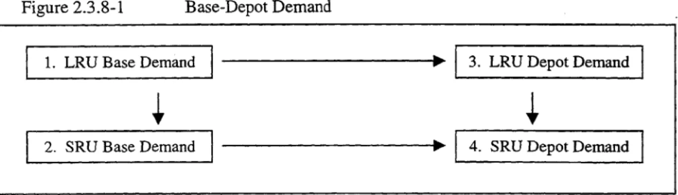
(Sherbrooke, 1992). Figure 2.3.8-1 displays a representation of the flow of materials through the system. Arrows represent the demand flows. From 1 to 2, the base requires

an SRU that it has in inventory, or if the base does not have the SRU in stock, it will be ordered from the depot, as is depicted from 2 to 4. From 1 to 3, the base needs a

completely new LRU, and the defective unit is shipped to the depot for repair. From 3 to 4, the LRU demands an on-hand SRU at the depot.

Figure 2.3.8-1 Base-Depot Demand

1. LRU Base Demand 3. LRU Depot Demand

A set of equations will be developed that can derive the SRU demand rates at the

base and depot, and the LRU depot demand rates from LRU base demand rates, m;. The

SRU demand rate for item i at base

j

multiplied by the conditional probability that the LRU will need SRUi for repair. Thus,

my = morojqj (2.3.8-3)

Since mi(1-ri;) represents demand for SRUj at basej that must be repaired at the depot,

the fraction of depot demand for SRUi resupplied to base

j

f

Mio

For SRU's in base repair/resupply, the number of units i at base j will be the pipeline (order-and-ship time and base repair time) plus the fraction of delays resulting from depot backorders of SRU i.

E(x, )= m, [(I- rj q0 + rjT

]+

Var(x,

)=

f,

)+

Depot LRU demand will be a function of all LRU base demand rates multiplied

by their associated probabilities that they cannot be repaired at the base.

I

moo =Y m(I o

(-

j=1

The fraction of demand at the depot for SRUi due to LRU depot repairs is

fio

For depot repair of an LRU, an SRU backorder with probabilityfio, could be delaying the repair, or delaying resupply to a particular base.

E(xo

)=

)

i=1 i=1

Var(xOO

)

Xf

f

)EBO(si

)+

moio)(238)

SRU depot demand rates will be a function of both LRU depot demand rates that

have a conditional probability of fault due to SRUj, plus SRU demand that, with a given probability, cannot be repaired at its base:

mi =m,,

(1

j=1

The fraction of LRU demand being resupplied to base j is

f

mo

Base repair/resupply for LRU's will be a function of three situations: the pipeline when there are no backorders (the order-and-ship time and base repair time), resupply delay due to depot LRU backorders, and repair delay due to base SRU backorders. Therefore, the mean and variance will be

E(xo, )= m; [(i - roj )00 + rj T,,

]+

f

jE(xOO

),

))+

|E(xij

]+

f,

fo,

As an example, consider a system of one depot supplying two bases. The

procurement manager must decide the most optimal way to purchase two separate LRU's where each LRU consists of two, non identical SRU's. Appendix D displays the list of information needed in the VARIMETRIC algorithm for this situation. Highlighted are those characteristics that must be approximated or assumed. The order-and-ship times from depot to base are not tabulated.

Appendix A.3 provides the detailed calculations. The METRIC method will be followed again. Expected backorders are calculated for varying stock levels, and procurement decisions are made based on marginal analysis of cost and expected backorders. A level of availability or a budget constraint is used to determine the final

stock levels across LRU families. While spreadsheet formulation was adequate for the previous example, a more realistic approach to determining optimum stockage policies requires the use of traditional command line computer programming.

2.3.9 Applications of VARIMETRIC

A computer model entitled OATMEAL (the Optimum Allocation of Test

Equipment/Manpower Evaluated Against Logistics) has been developed by Kaplan and Orr (1985). This sophisticated algorithm establishes optimal inventory policies for three-indenture items by focusing on operational availability. According to Sherbrooke (1992), the armed forces have applied an ordering algorithm to spares planning. The US Air Force has used a VARIMETRIC program called Aircraft Availability Model to estimate

spares budgets, the US Army has an alogorithm called SESAME (Selected Essential-Item Stockage for Availability Method), and the US Navy has a model titled ACIM

(Availability Centered Inventory Model). Several aircraft manufacturers in Europe use a VARIMETRIC-based model called OPUS, developed in Sweden. IBM has used an

inventory planning program to manage its spare parts for a four-echelon system consisting of over 200,000 stock keeping units (SKU). After implementation of its program, IBM has reduced its inventory investment by almost 25% for a savings of $0.25 billion (Sherbrooke 1992).

2.3.10 Comparison of Inventory Policies

Muckstadt and Thomas (1980) compared three types of inventory models: level decomposition, item decomposition and a "days of supply" system. The level

decomposition policy maintains an aggregate service measure at a constant level where each echelon will minimize their stock investment to meet a given service level goal. Tradeoffs occur between system performance level and system investment. The item decomposition, or METRIC, approach already described extensively in this thesis set stock levels for all items at all locations according to an optimized ordering plan. The "days of supply" approach allocates stock according to a specified time period. This policy is the most widely used system in practice, although it did not perform well enough to be included in their conclusions.

When measured against the level decomposition approach in their experiment, the METRIC approach consistently required less investment than the level decomposition approach for the same level of performance, with some items requiring only half the inventory. In addition, they found that the larger the number of low-demand items and tighter the budget constraints, the better the performance of a METRIC solution.

All inventory planning systems require some form of control through the use of

information technology. It was determined that the computation cost of implementing a METRIC system is comparable to that of the level decomposition or "days of supply"

system. Since the "days of supply" approach is not comparable, and item decomposition consistently outperformed level decomposition, the METRIC inventory planning system is the best solution.

2.3.11 Multi-Echelon Extension

A theoretical study by Malec and Steinhorn (1980) has shown that infrastructure

design can reduce the number of required reparables spares in a system. Extending the multi-echelon system to base, depot, and sub-depot facilities, the same service level in a base-depot configuration will hold more spares compared to a sub-depot design.

The sub-depot design is shown in Figure 2.3.11-1. When an item fails at a base, an on-site spare is instantly provided. The on-site spare is replaced with a sub-depot spare, which is replaced by the depot spare. The failed unit is shipped to the repair facility, where it is repaired and transported to the site's depot. The sub-depot configuration ensures a higher probability of the depot providing a spare when one is needed. Although the following analysis does not consider an LRU/SRU family, the model can be extended to include component part failures. Using the Poisson distribution for item demand rates, it was shown that under a system of 15 depots and 75 bases, the depot should hold 270 spares to satisfy an overall availability constraint greater than

sub-depot serving five bases, 201 total spares are required for the same 99.9%service level. This system redesign represents a 25.6% reduction in inventory.

Figure 2.3.11-1 Sub-Depot System Design

Despite the quick inventory reduction, a complete analysis of the sub-depot configuration should include the cost of added infrastructure weighed against the benefits of holding fewer inventories. For a transit agency located in a city where land is

expensive, the addition of a new warehouse as a sub-depot facility can mitigate the advantages of purchasing fewer spares.

2.4 Supply Chain Management

Supply chain management is a business philosophy reflecting a new paradigm in operations to dismantle the barriers that exist in the manufacturing and distribution of goods from raw material to end consumer. A typical configuration of supply chain links begins with the raw material provider. Product flows to a manufacturing or processing

plant and is transported to a distribution center. From there, product is shipped to a wholesaler and finally to a retailer. Sharing information between these links can improve

operations. A study of the apparel industry by Kurt Salmon Associates shows the effect of information sharing on lead-time, product sales and returns on investment (Hammond and Kelly, 1990). The improved supply chain allowed apparel retailers, wholesalers, and manufacturers to produce and sell products more efficiently in an environment where fashions change rapidly.

For the apparel industry, long lead-times produced a wealth of unwanted materials and poor customer service levels. In other industries, long lead-times result in an

overabundance of safety stock. Safety stock exists to leverage against uncertain demand during a lead-time and the variability in the lead-time itself. New management

techniques have attempted to control the lead-time by forming channel partnerships. Through partnerships with suppliers, savings can be realized via improved service levels,

reduced operating expenses due to fewer transaction costs, and reduced inventory levels. In the Health Care Industry, Baxter, a supplier of consumable hospital goods, has initiated a stockless program to offer hospitals commonly used medical supplies such as latex gloves and IV solutions as the prime vendor. In the past, bidding wars were constantly fought over a difference in price of $.03 for consumable hospital products (Byrnes, 1993). To transform these relationships, Baxter established new alliances with hospitals that focused on consumer needs and mutual values. As a result, the

participating hospitals eliminated a large amount of inventory, cleared stockroom space for other supplies, and cut a portion of its materials management labor costs.

Intercompany operating ties, such as Baxter's system, are seldom as simple to implement as they appear (Byrnes and Shapiro, 1991). Awareness of risks and rewards is commonly overlooked when addressing a potential partner. Understanding the internal changes necessary, the communication between parties, and the importance of a common strategic view are important areas of consideration. Of utmost significance, a transit agency attempting to implement new supply chain management practices must be lead by management that is familiar with logistics and understands the orientation and goals of its organization.