COLOR-NAMING
by
Rony Daniel Kubat
B.S. Computer Science, MIT 2001 B.S. Mechanical Engineering, MIT 2001
Submitted to the Department of Electrical Engineering and Computer Science
in partial fulfillment of the requirements for the degree of Master of Science in Computer Science and Engineering
at the
MASSACHUSETTS INSTITUTE OF TECHNOLOGY February 2008
@ Rony Daniel Kubat, MMVIII. All rights reserved. The author hereby grants to MIT permission to reproduce and distribute publicly paper and electronic copies of this thesis document
in whole or in part.
Author... ... .:;.. Department of Electrical Engineering and Computer Science
October 1, 2007 Certified by ... ... .. 06K. Roy Associate Professor Thesis Supervisor A ccepted by ... .... ,... ... Terry P. Orlando Chairman, Department Committee on Graduate Students v ·
-, !.• . ·<: . ' • . ..
A~c~IVES
OF TEQMNOLOGYby
Rony Daniel Kubat
Submitted to the Department of Electrical Engineering and Computer Science
on October 1, 2007, in partial fulfillment of the requirements for the degree of
Master of Science in Computer Science and Engineering Abstract
Humans are sensitive to situational and semantic context when applying labels to colors. This is especially challenging for algorithms which attempt to replicate human categorization for communicative tasks. Additionally, mismatched color models between dialog partners can lead to a back-and-forth negotiation of terms to find common ground. This thesis presents a color-classification algorithm that takes advantage of a dialog-like interac-tion model to provide fast-adaptainterac-tion for a specific exchange. The model learned in each exchange is then integrated into the system as a whole. This algorithm is an incremental meta-learner, leveraging a generic online-learner and adding context-sensitivity. A human study is presented, assessing the extent of semantic contextual effects on color naming. An evaluation of the algorithm based on the corpus gathered in this experiment is then tendered. Thesis Supervisor: Deb K. Roy
I have been granted a great opportunity to work among such a talented and interested cadre as I have found at Cognitive Machines, the research group where I've spent the last two years. First, I would like to thank my intrepid advisor, Deb Roy who has been all I want from a mentor, providing inspiration and guidance but also freedom and trust. I also want to thank the National Science Foundation and the American taxpayer, without whom it would have been impossible for me to find my home at the Media Lab amongst the cogmac'ers. Many thanks to all the members of cogmac, with whom discussions have been informative and inspiring and critiques strengthening. Special thanks are deserved by Dan Mirman who helped tremendously in the design and analysis of the experiment described here. Finally, thank you to my family: Peter, Hadassa and Emilie who have been unyielding sources of support, encouragement and creative inspiration.
I
CONTENTS
1 Introduction 13
1.1 Context Sensitivity ... ... 14
1.2 Motivation and Inspiration . ... 14
1.3 Straddling Two Worlds ... .. 15
1.4 Outline ... ... 15
2 Background and Related Work 17 2.1 A Brief Introduction to the Science of Color . ... 18
2.1.1 Biological Basis ... ... 19
2.1.2 Oppositional Color Theory . ... . 20
2.1.3 Color Spaces ... .... 21
2.2 Color Categorization ... .... 24
2.2.1 ... in the Cognitive Sciences . ... 24
2.2.2 Computational Models . ... 25
2.3 Concept Spaces, Context-Sensitivity and Linguistic Hedges 27 2.4 Meta-Classification Techniques . ... 28
3 The Context Dreaming Algorithm 31 3.1 Context Dreaming as Meta-Classifier . ... 33
3.2 The 50,000 Foot View ... ... 33
3.3 Terminology, Parameters and Structure . ... 34
3.4 Phase I - The Wake Cycle . ... . 36
3.5 Phase II - The Sleep Cycle . ... 37
3.6 Expected Performance and the Effect of Parameters .... . 38
3.7.2 Refined Context Intersection ... 41
3.7.3 Training a Filter ... 41
3.8 Discussion ... 42
4 Context Effects on Color Naming 45 4.1 Experiment ... 46
4.1.1 Participants ... 46
4.1.2 Equipment ... .. 46
4.1.3 Stimulus-selection ... 47
4.1.4 Color-Survey Task ... 48
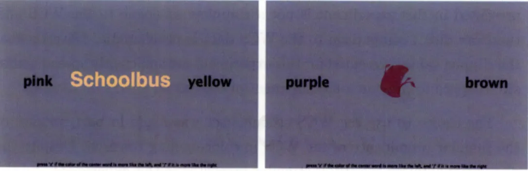
4.1.5 Binary Forced Choice Task . ... 50
4.1.6 Naming Task (Surround Context) . ... 51
4.2 Results and Discussion ... . . . .. . . . . 52
5 Evaluating Context Dreaming 59 5.1 The Implemented System ... 60
5.2 Procedure ... ... 64
5.3 Comparison Classifier ... ... . . 64
5.4 Results and Discussion ... .... ... . . 64
6 Conclusion 69
A Image stimulus used in the experiment 73
I
LIST OF FIGURES
2.1 The spectral distribution of a few common illuminants... 19 2.2 The CIE XYZ color matching functions and the xy
chromatic-ity diagram showing the sRGB gamut and white-point... . 22 3.1 Boxology of the Context Dreaming Wake cycle algorithm. .. 36 3.2 Boxology of the Context Dreaming Sleep cycle algorithm. .. 38 4.1 Screenshots from the experiment: Naming and membership
tasks ... ... 50
4.2 Screenshots from the experiment: Forced choice tasks . . . . 50 4.3 Results of the binary forced-choice tasks... 54 4.4 Average response times for the binary forced choice tasks and
the surround context task. . ... . 55 4.5 Schematic for a model which may explain the binary
forced-choice results. . ... ... 57 4.6 Results of the surround-context naming tasks. ... . 58 5.1 The effects of - and w on Context Dreaming performance and
library size. ... ... 66
3.1 Parameters to the Context Dreaming algorithm and their
con-straints . ... . ... . ... ... . 35
4.1 Demographics of the study participants. . ... . 46
4.2 The eleven basic color terms of the English language... . 47
4.3 Results of the ambiguous-color calibration task... 49
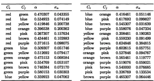
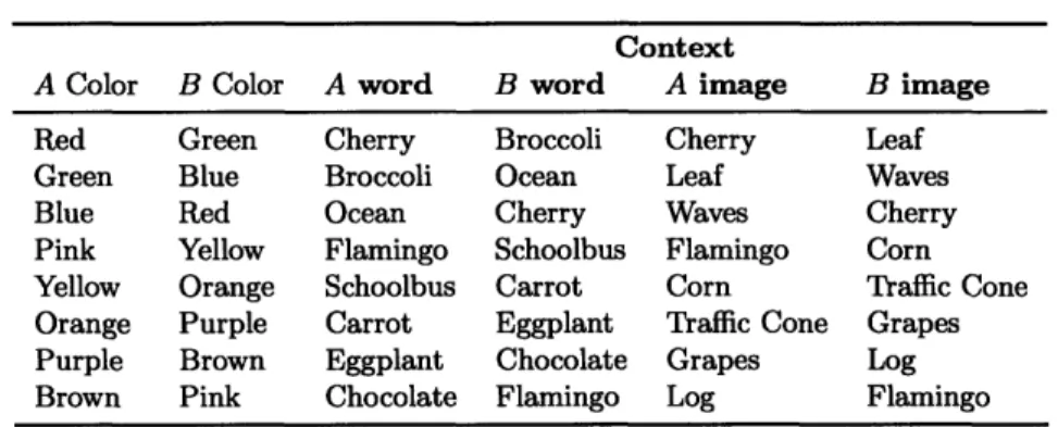
4.4 Color pairs used in the experiment and the word and image contexts used ... . .. . .. . ... 52
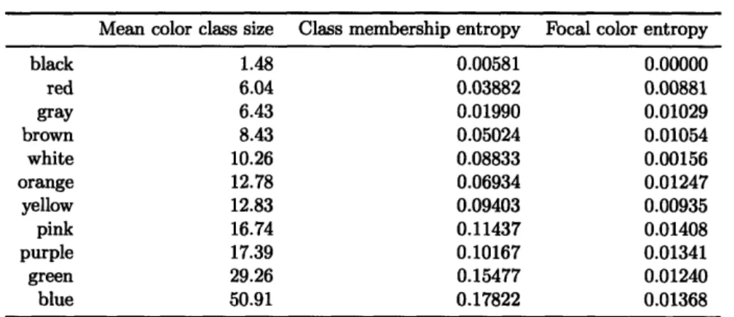
4.5 Mean color class size and average information entropy for color swatches in the color foci and color class tasks . . . 53
discovering colors for the first time: red was quite cheerful, fire red, but perhaps too strong. No, maybe yellow was stronger, like a light suddenly switched on and pointed at my eyes. Green made me feel peaceful. The difficulties arose with the other little squares. What's this? Green, I said. But Gratarolo pressed me: what type of green, how is it different from this one? Shrug. Paola explained that this one was emerald green and the other was pea green. Emeralds are gems, I said, and peas are vegetables that you eat. They are round and they come in a long, lumpy pod. But I had never seen either emeralds or peas. Don't worry, Gratarola said, in English they have more than three thousand terms for different colors, yet most people can name eight at best. The average person can recognize the colors of the rainbow: red, orange, yellow, green, blue, indigo, and
violet-though people already begin to have trouble with indigo and violet. It takes a lot of experience to learn to distinguish and name the various shades, and a painter is better at it than, say, a taxi driver, who just
has to know the colors of traffic lights.
I
I
INTRODUCTION
Anjou Pear. Frolic. Capri. Bagel. Heartthrob. Camelback. Flip through the catalog of paints at your local hardware store, and these are the kinds of names you'll find, each a coding for a specific combination of inks. None of these terms are universally used for the subtle hues of the spectrum. Calling your mother and telling her that you're painting your bedroom "summer day" won't quite convey the off-peach tone. Color, though, is one of the key ways we refer to things in our world. What kind of wine would you like with your sirloin? Describe the car that left the scene of the crime...
Somehow, through multiple layers of perception and cognition, we trans-form a patch of light hitting our retinas into a label; a color name. And what's more, that name is simultaneously stable to radical shifts in lighting, and malleable to the situation. In the sciences, color has been a window into the mind. By carefully controlling the light striking the light-sensitive cells of the eye, we have learned about neural coding at the lowest levels of perception. By surveying languages of the world, we have discovered univer-sals in the categories of color and hypothesized about what these univeruniver-sals mean for the evolution of language and of thought. Engineers have arrived first from a different standpoint: how can colors be reproduced accurately. How can we represent them compactly? Transmit them? And now, how can
we categorize them?
This thesis touches on both the science of the human perception of color and the engineering of distinguishing one color from another, and through this investigation connects with a broader issue of classification with a frame of reference: contextual dependence.
1.1
Context Sensitivity
Politicians complain that their words are quoted out of context; that a phrase, removed from the particulars of situation, takes on meaning mismat-ched-or worse yet, contradictory-to what was intended. Word meanings are mutable to the context of their use. What's meant of "weight" when comparing a heavy feather to a light bowling-ball? What of discipline when a father speaks to his son or a warden to a prisoner? Any model of word meaning must take context into account, but formulating a general model is an enormous undertaking. Here, I grasp at one narrow manifestation of a context's effect on meaning in the domain of color naming.
1.2
Motivation and Inspiration
The work presented here was initially motivated by a specific application in linguistic grounding, the connection of words to the real world [34]. Trisk is a robot at the MIT Media Lab designed to interact with objects placed on a table before it, and to communicate about them with humans by speech. Trisk visually identifies objects of interest by segmenting camera input based on color.' We found this color segmentation fragile to changes in lighting conditions, shadows, and the specular reflections of the objects in view. The work of this thesis began in part as a venture to find a robust color-based method of image segmentation. Trisk uses color terms to refer to objects and can respond to imperatives such as "put the green one to the left of the blue one." Like an art dealer describing a painting, Trisk must match color iComputer vision is not the focus of the work presented in this thesis, though for those interested, a survey of color-based segmentation techniques can be found in [8].
to label. It's in this more direct use of color classification that the system described here will likely find more immediate use.
The name of the context-sensitive classification system I developed is Context Dreaming. The dreaming half of the name comes from one of the most direct inspirations for the system. Daoyun Ji and Matthew Wilson of the Picower Center for Learning and Memory at MIT recently published a paper [18] supporting a proposal for memory consolidation. In this paper, they report rats playing back memories while dreaming. Perhaps the kernel of this notion of memory playback during an "off-line" time could be directly implemented by a computer?2 Thus came the two-phase interrogative
learn-ing model that Context Dreamlearn-ing employs. Humans also appear to learn by two different routes. There is a fast "in-context" system, and a slower learning mechanism which consolidates and integrates multiple experiences
[25].
1.3 Straddling Two Worlds
This thesis spans both cognitive science and computer science. The contri-bution to the cognitive sciences are the results of an experiment I performed to assess semantic contextual influence on color categorization. These re-sults confirm that even abstract context can affect low-level perception, and raise questions about the mechanism that causes this effect. In the com-puter sciences, I have designed a meta-classification algorithm which takes advantage of a real-world interrogative interaction model and can transform online-learners into context-sensitive online-learners.
1.4 Outline
The next six chapters describe the framework I designed to add context sensitivity to online classifiers. The next chapter begins with a short review of the science of color-its representation and partitioning--and describes
2
The Context Dreaming algorithm shares the nomenclature of the wake-sleep algorithm for neural-networks[17], but not the mechanics.
the relevant work which frames this thesis. Chapter 3 describes in detail the Context Dreaming algorithm. Next is a report of the experiment I designed and performed to quantify some semantic context effects on color naming. The corpus gathered in that experiment is used to evaluate the Con-text Dreaming algorithm in Chapter 5. Finally, I conclude with a proposal for future directions for this line of research.
CHAPTER
2
I
BACKGROUND AND RELATED WORK
The study of how people select names for colors has a rich history. Color can be seen as a window into cognition-a direct route to address at least one aspect of the nature versus nurture debate. Are color labels independent of language and tradition or do upbringing and culture directly shape percep-tion? The goal of this chapter is to briefly introduce the key concepts which frame this thesis, and provide context for the choices I have made. The first part of this chapter discusses the science of color and its perception by hu-mans, especially focusing on representations of color. It is on this substrate that parts of this thesis are built. The second part of the chapter gives a con-densed introduction to research on color-categorization, and describes some related work on computational models of color-naming. The final part con-siders some related work on context sensitivity and meta-classifiers. Those familiar with these topics may skip the sections (or the chapter) entirely, without losing critical information about Context Dreaming, its evaluation, or the context-dependent findings discussed in Chapter 4.
2.1
A Brief Introduction to the Science of Color
Imagine you are sitting at your kitchen table at dusk, a basket of fruit before you. A clear sky outside illuminates the room dimly, while an incandescent lamp overhead casts a pool of light upon the bowl. What happens when you "see" the apple on your desk? Light from the sky and the lamp strike the surface of the apple, where it is filtered and reflected into your eyes. There, the light is absorbed by your retina and translated into signals which travel to your brain. Somehow, you decide the color of the apple is red. I will use this simple example to help introduce some key concepts which will take us from the illuminant to the retina.Light is a continuous spectrum of electromagnetic energy. The range of the spectrum visible to the human eye are the wavelengths between 300nm and 700nm. Purely spectral light-monochromatic light composed of one particular wavelength-is, in a sense, a pure color. Rainbows are made from these pure colors. Partitioning the visible spectrum into colors, we see violet at 300nm range though deep red at the 700nm. Most sources of light, though, radiate a distribution of the spectrum rather than a specific wavelength, a bumpy but continuous spread of energy. The most idealized case is that of a black-body, a material whose spectral radiation is defined only by its temperature and related by Plank's Law:
2hc2 1
I(A, T) = hc 1
e AkT -
1
What we refer to as "white" light is a complex distribution across the spectrum-in fact, there is no single standard for white light. The Interna-tional Commission on Illumination (known more commonly by the acronym for its French name, the Commission internationale de l'dclairage, CIE) has defined a number of standard illuminants approximating common sources of white light. Figure 2.1 shows the spectral distribution of a few of these illuminants, including a black-body source. These standard illuminants are the basis for the white points used by the color representation standards discussed below.
Spectral Distributions of Some Standard Illuminants
Figure 2.1: The spectral
distribu-tion of a few common illuminants.
The smooth curve is the idealized black-body radiation of a 65000K source. The bumpy curves are exper-imentally measured distributions of the CIE standard D65 (sRGB and
television, western Europe daylight)
and A (incandescent) sources.
300 400 500 600 700 800 900
Wavelength (nm)
Humans compensate for the radical spectral differences of white light, a phenomenon called color constancy. Once you've adjusted to the ambient lighting, a sheet of paper looks white, whether seen at dusk or at noontime on a sunny day. Color constancy is a perceptual effect. Computational color constancy, sometimes called white-balancing, is a long-studied problem. See
[1] for a comparison of different algorithms.
The scene in the kitchen has two primary light sources: the sky, which has a bluish tint, and the incandescent bulb with a yellowish tint. We can model these light sources with the CIE illuminants D65 and A, respec-tively. Light hitting the apple is a superposition of these sources. When this light strikes the surface of the apple, it is selectively absorbed and reflected-transforming the incident spectral distribution into the final one which reaches your eyes.
2.1.1 Biological Basis
Light striking the human retina is absorbed by one of two types of light-sensitive cells. One of these types, rods, are light-sensitive to dim light, but not used to distinguish colors and will not be discussed here further. The color-sensitive type, known as cone cells, come in three varieties,1 each of
'Colorblindness is a genetic limitation in which only two types of cones are present. There is some evidence of human tetrachomats (people with four types of cone cells, with four distinct photopigments), but as of this writing, very few have been found.
... Blacody (6500 K) .-- Blaclody (9300 K) -- CIlE D65 - - -CIE A I S '• . .·· · , •· 30. 250 200 . 150 dr 100 50 oo """ Y
which uses a distinct photopigment to selectively absorb light spectra. The excitation of a cone cell is a function of both the incoming spectra and the absorption of the cell's photopigment:
L(A) = /I(A)a(A)dA
where L(A) is the cell's response, I(A) is the spectral power of the incident light and a(A) is the absorbance of the cone cell's photopigment. The human visual response to color can thus be quantified by the rates of excitation of the three types of cone cells. A consequence of this tristimulus representation of color is metamerism: two distinct color spectra may result in the same responses by the three cone types.
2.1.2 Oppositional Color Theory
The earliest models of color were split into two camps: Isaac Newton leading from a physical substrate based on color spectra, and Johann Goethe from empirical experiments on human perception. Goethe describes his theory in
Theory of Colours[41]. Introduced in the book is Goethe's color wheel, a
symmetric ring where colors are "arranged in a general way according to the natural order, and the arrangement will be found to be directly applicable
[... ]; for the colours diametrically opposed to each other in this diagram are those which reciprocally evoke each other in the eye."2
Goethe's notion that colors are arranged in oppositional pairs anticipated the opponent process model proposed by Ewald Hering [16], where colors are encoded as the difference between tristimulus values. As a consequence, red and green oppose each other, as do blue and yellow.
The debate between opponent models and tristimulus models carried though the 1800s, with Hering and Hermann von Helmholtz as prominent proponents of each respective theory. Today's consensus is a combination of both theories, tristimulus tied to low-level perception and opponent colors at higher levels of cognition.
2
paragraph #50
2.1.3 Color Spaces
The desire to faithfully capture and reproduce color gave rise to the question of how to accurately and efficiently represent color. A color space is a method of mathematically encoding color. The gamut of a color space is the set of colors representable in that space. Discussed here are a few of the prominent color spaces used for scientific and color reproduction purposes, all of which are represented as a triple of numbers. Formulae for converting between the color spaces described here can be found in [43].
LMS
The three types of cone cells in the human eye contain photopigments which, at first approximation, absorb light in long, medium and short wavelengths. The LMS (long-medium-short) color space gets its name from this fact. LMS triples represent the excitation of the three types of cone cells and so LMS space is most closely grounded to the physiological response of human vision. Nevertheless, LMS is almost never used in either color capture or reproduction due to mismatches in the sensitivity between the three types, the linearity of their measure, and the difficulty relating LMS values to color reproduction by screen or printing. LMS space is linearly related to XYZ (see below). The LMS gamut spans all visible colors.
XYZ and its variants
In 1931, the International Commission on Illumination (CIE) formulated a standard representation of color named XYZ. XYZ was one of the first scientifically defined color representations and has remained the basis of many of color spaces later developed. Each of the three components of XYZ (which roughly correspond to red, green and blue) are linearly tied to the human LMS tristimulus responses.
The XYZ standard is based on a color matching experiment in which subjects were presented with two patches of color, separated by a screen. On one side was a test color of fixed intensity; on the other, a combination of three monochromatic sources whose brightness could be adjusted. By
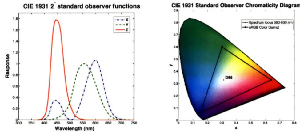
CIE 1931 2* standard observer functions CIE 1931 Standard Observer Chromaticity Diagram
a
Wavelength (nm) x
Figure 2.2: The CIE XYZ color matching functions and the xy chromaticity diagram showing the sRGB gamut and white-point.
manipulating the primaries, subjects found a metameric color which could be quantified by the intensities of the three primaries. From this data, CIE created the standard observer color matching functions x, y and x, each of which is a function over wavelength A. A color in the XYZ color space can then be defined by the equations:
X = I(A)x(A)dA, Y = I(A))(A)dA, Z = I(A)2(A)dA
)0 0
Figure 2.2 shows the CIE XYZ color matching functions.
An XYZ triple encodes both the color of light as well as its intensity. A standard decoupling normalizes x and y into a new space xyY defined as:
X
Y
= X+Y+Z'
y X+Y+Z
The two normalized chromaticity coordinates x and y encode color while the third coordinate scales for intensity. The locus of monochromatic light, swept through the spectrum of visible colors traces a horse-shoe shaped arc whose inner area contains all colors visible to humans. Points outside this arc represent ratios of excitation impossible for the three types of cone cells. They are called imaginary colors.
( 22)
0.9 I
3.
RGB and its variant sRGB
The reproduction of color for television and computer displays is by com-bination of three color primaries of red, green and blue. The brightness of each primary can be represented as a normalized number in the range [0, 1]. The chromaticity of the three primary colors forms a triangle which defines the gamut of the RGB space. One other factor completes an RGB space: a white-point. This XYZ triple, corresponding to the "color" of white light, provides a parameter to a transformation which can be used to adapt the RGB space to the color temperature of the viewing environment.
Relevant to this thesis is one particular RGB standard named sRGB, developed by Microsoft and HP to standardize monitors and printers. The chromaticity of the sRGB primaries are based on standard phosphors for CRT displays and the white-point set at CIE D65. Figure 2.2 shows the spectral locus and the gamut and white-point of the sRGB standard.
Perceptually linear color spaces and CIE L*lIf
A problem with the color spaces described above, especially with regards to color naming, is their perceptual non-linearity. Euclidean distance in XYZ or RGB is not comparable to perceptual distance. For each visible color in the xy chromaticity diagram, there is an ellipse of nearby colors which are perceptually indistinguishable. The size of these MacAdam ellipses [23] varies, smallest in the blues and growing larger toward the greens and reds. There have been a number of attempts to define color spaces for which the MacAdam ellipse stays approximately the same size throughout the color space. Moreover, the goal of these color spaces is to make Euclidean distance a parallel measure of perceptual distance gathered experimentally.
CIE ULa*b* was the CIE's 1976 attempt to define a color space that balanced perceptual linearity with straightforward conversion to and from XYZ. The three components of a CIE L*a*b* triple are luminance (a measure of brightness) and two color-difference chromaticity values a* and b*, which roughly encode differences between green and magenta, and blue and yellow, respectively. In that sense, though a triple, CIE L*a*b can be considered
an opponent color space. The * in CIE L*a*b* notes that each component is converted from XYZ with an exponential-better matching human loga-rithmic response. L* values vary between zero and one hundred; a* and b* values vary in the range [-128, 128].
Although much closer to perceptually linear than XYZ, CIE L*a*b* is not perfect. Other perceptually linear color spaces have been proposed, includ-ing the OSA Uniform Color Scales Samples [31], CIE L*iflv, and NPP [22]. Mojsilovic describes a non-Euclidean distance metric which compensates for irregularities in CIE L*a*b* [29].
2.2 Color Categorization
This section summaries some previous work in color categorization both in the cognitive and computer sciences. In the cognitive sciences especially, color classification has been an active field of research, perhaps because of the ease with which experiments can be created and replicated as well as the close connection between raw stimulus and semantic structure.
2.2.1 ... in the Cognitive Sciences
In 1969, Berlin and Kay published Basic Color Terms: Their Universality
and Evolution[3], a collection of their research about the naming of colors
across cultures and languages. In their key experiment, a standard palette of color chips were named by participants speaking different native languages. Language-specific aggregate mappings from colors to names were collated from this data. Berlin and Kay put forth two hypotheses: that (1) there is a restricted and universal catalog of color categories and (2) languages add these categories in a constrained order. Languages with only two color terms would have terms for black and white. Languages with three have black, white and red. Those languages with four have terms for the former three, plus green or yellow. The hierarchy for color terms proposed was:
purple
white green pink
< red < < blue < brown <
black yellow orange
gray Data collection for this experiment has continued through the World Color Survey (WCS) [19] and a recent analysis of this data argues that the parti-tioning of color categories follows an optimal partiparti-tioning of the space [33], lending strength to the argument that human partitioning of color space into categories is in large part bound to the physiology of human vision. Low-level color perception, though, is influenced by higher levels of cogni-tion, including memory [13]. By using swatches to present colors to study subjects, the WCS researchers attempted to remove any contextual influ-ences on color naming. John Lucy, in [14], though, argues that the three dimensions of color presented in the WCS stimulus array are insufficient for color naming. Namely, they were lacking in degrees of luminosity, re-flectance and luster. Furthermore, he argues that color-naming can never be fully detached from referential context and range.
Most natural kinds which people classify have distinct borders of mem-bership. Not so with color. Children only start using color terms with their full referential meaning between ages four and seven despite being able to discriminate colors in dimensions of hue, saturation and brightness [4]. The categorization we take for granted is a hard problem.
2.2.2 Computational Models
There have been a few computational models for color naming. Mojsilovic in [29] describes a system to name an image's dominant colors. The image is first segmented into regions by color and texture, then each color region is named by taking the region's CIE L*a*b* color value and finding the closest prototype in the ISCC-NBS3 dictionary [24] using a distance metric based
on Euclidean distance. Nurminen et al. [32] also name the dominant colors of an image. Image pixel values are converted to CIE L*a*b* space, then
3
clustered by k-means and agglomerative clustering. Names are assigned to cluster centers by using unmodified Euclidean distance metric to find the nearest color prototype in a dictionary. An open-source javascript based color naming tool by Chirag Mehta [26] uses a dictionary of color terms combined from wikipedia, Crayola and others.4 The distance metric used combines RGB values as well as hue, saturation and lightness.
Lammens [22] uses a Gaussian model to select the best color term in a neurophysiologically-derived color space (NPP). He describes a way of combining color labels near the border between color categories to make complex color terms such as "reddish-yellow" and "somewhat blue".
Steele and Belpaeme's target article [39] about getting artificial agents to coordinate color categories by communication (see also [2]) included a color-naming model related to Lammens. The agents simulated in this experiment categorized colors in CIE L*a*b* by using adaptive networks of locally reac-tive units, a system similar to radial basis function networks. Units of a network have a peak response at one specific color, with exponential decay around it; the final output of a network is the sum of the individual units. Each color category is represented by a network and a categorization made by the network whose response is highest.
Recently, Mengaz et al. [28] demonstrated a model in which each point in the gamut of the OSA uniform color samples is assigned fuzzy mem-bership to the eleven basic color terms. Memmem-bership values were assigned experimentally for the OSA samples and interpolated for other points in the space.
One of the problems for all of the above computational color-naming models is that none take into account human color-constancy. It can be argued that white balancing can implemented as a preprocessing step before submitting a color to be categorized, but the color representations chosen for each of the above models attempt to lock colors to specific physiological responses, so preprocessing the image in a sense betrays the impetus for each respective color representation. An alternative representation is the CIE
4A list of different color name dictionaries can be found at
http: //wvw-swiss.ai.mit. edu/t jaf fer/Color/Dictionaries.html
CAM color appearance model [30], which attempts to model the perceptual effects of surround, adaptation, illumination and white-point, predicting the appearance of a given color. Even with perceptual effects accounted for by white-balancing or a color appearance model, none of the above color-naming models take into account the semantic context of the color being named, something this thesis hopes to address.
2.3 Concept Spaces, Context-Sensitivity and
Linguis-tic Hedges
Peter Giirdenfors proposes a three-layered model of cognition in [11] split between Associationist (connectionist), Conceptual (geometric) and Sym-bolic (propositional) representations. The central, geometric, component Girdenfors names conceptual spaces. Abstract concepts, such as robin, can be represented as a high-dimensional region in a geometric space with di-mensions such as "can-fly" and "has-wings". The region representing robin lies within the region for bird. Reasoning and inference about concepts can then be transformed into a geometric problem where geometric algorithms can be applied [12]. Conceptual spaces have been applied to both text [38]
and vision [7] problems.
In Gihrdenfors' model, context effects can be seen as a selective scaling of the conceptual dimensions. On the farm, the concept for bird would scale up the visual "has-wings" dimension, while at the dinner-table, the "tasty" dimension would be emphasized. Applied to color-naming, the context of wine would scale the salient color dimensions to bring a deep purple into the region labeled "red".
To communicate about concepts in the word, we must have a shared common ground with our conversational partner. Sometimes, though, it is difficult to determine this shared conceptual space, especially if either the two partners' models greatly differ, or if the word used refers to intangible or invisible things. Arriving at a shared conceptual understanding is the subject of linguistic and cognitive research [6, 15, 9]. Related to this work are
linguistic hedges [21], using fuzzy terms like "somewhat brown" or "reddish" to attenuate the meaning of a word or phrase. Hedges are frequently used in referential negotiations. The Steele and Belpaeme target article mentioned earlier connects many of the concepts discussed here: colors are classified by independent artificial agents, who come to a shared understanding of color terms through communication.
2.4 Meta-Classification Techniques
There is a fair body of research about techniques for combining classifiers to increase their predictive power. This class of techniques, in which base classifiers (sometimes called classifier stubs or weak learners) is called meta-classification. The most straightforward of these techniques is voting [20], wherein a number of stub classifiers each make an independent classification and the majority class is chosen as a final result.
Stacking [42] is a generalization of voting where each stub classifier is assigned a weight, and final classification is a result of the weighted vote of the stubs. The weights assigned to the stubs are chosen to minimize error in cross-validation. Stacking is a batch-learning technique due to the weight selection by cross-validation. Bootstrap aggregation (Bagging) [5] creates multiple copies of the training set by drawing samples with replacement. These new training sets are used to create a cohort of stub classifiers whose majority vote is reported as the final classification. Bagging is essentially a smoothing technique, averaging stub classifiers whose decision boundaries are sensitive to training data. Another technique which replicates data is the Decorate algorithm [27]. In this approach, data with fuzzy class labels is artificially generated from the training set. This artificial data is used to train stub-classifiers which are combined by voting.
In boosting [36, 37]), each iteration of the algorithm adds a weak learner trained on a weighted dataset, where those examples misclassified by the previous iteration are more strongly weighted. There are a variety of algo-rithmic variants of boosting, best known of which is perhaps AdaBoost [10]. All of the techniques mentioned above are batch learners. A labeled
training set is processed to create a meta-classifier, which remains static for all future classifications. To process new training data, these classifiers must retain their entire original training set. The algorithm described in this thesis does not suffer from this drawback-learning occurs incrementally rather than in batch.
CHAPTER
3
THE CONTEXT DREAMING ALGORITHM
This chapter describes the Context Dreaming algorithm in detail, discussing its operation, critiquing its model, describing its theoretical performance and discussing variants of the algorithm.
Context Dreaming is designed to take advantage of a particular interac-tion model: one of discrete "interrogainterac-tions." An example will help clarify what I mean. Imagine an automatic telephone troubleshooter for a com-puter company. A customer calls and describes a problem with a recently purchased product. The automatic troubleshooter can be seen as a so-phisticated classifier, asking questions of the customer and listening to the complaints in order to find the most accurate classification of the problem. Ideally, we'd want the automatic troubleshooter to learn from customers, both within the bounds of a single call (by cup-holder, the customer means compact disc tray) and by aggregating many calls (a whirring noise and smell of burnt hair is likely a power-supply problem). Essentially, there is local, in-dialog fast adaptation where joint definitions are negotiated ("The cup-holder." "The CD tray?" "The thing that slides in and out." "Okay.") and global learning, where the results of multiple conversations are aggre-gated to help speed the diagnostic process and obtain more accurate results in future dialogs.
This interrogative interaction model is common in real life, and in fact is critical whenever two parties are referring to a shared concept or item. What you mean by "democracy" is likely subtly different from what I mean by "democracy." If you use the term in a way I find surprising, I can ask you to clarify and update my local definition for our conversation. My personal interpretation can remain intact, but we can continue with a shared com-mon understanding. The next time "democracy" comes up in conversation between us, I can recall our shared meaning and proceed without confusion.
A more concrete example--one which motivates the evaluation described later-is that of two parties negotiating the meaning of color terms. Imag-ine you are sitting across a table from anther person. On the table are two objects whose colors you would describe as cyan and purple. Your interrog-ative partner says, "Hand me the blue one." Which one did he mean? For you, there is no clear example of a "blue one" so you are forced to decide between the two objects present. Let's say you hand him the cyan object and get the reply, "Thanks." You've now learned that for purposes of this interrogation (and perhaps for future conversations with this partner) colors that you classify under the term "cyan" can also be classified as "blue." An understanding of color has been negotiated.
The dialog model for classification is intimately tied to the functioning of the Context Dreaming algorithm. There are two distinct phases of oper-ation, one which occurs before and during a dialog, and one which occurs afterward. The first, the online wake cycle, is analogous to the automated troubleshooter's conversation with a single customer or the negotiation of blue and cyan colors. This phase has a beginning and end, and its duration is much shorter than the lifetime of the classifier (which can continue indef-initely). During the second phase, the offline sleep cycle, knowledge learned during a dialog is incorporated into the global model by replaying any new training examples. For our earlier example, it's here that the troubleshooter will generalize from "this customer calls the CD tray a cup-holder" to "some-times, customers will call the CD tray a cup-holder."
3.1
Context Dreaming as Meta-Classifier
There are a number of techniques that can be used to combine machine classifiers in ways which improve performance, both in speed and accuracy. Perhaps the simplest example is a voting classifier. In this meta-classifier, a collection of sub-classifiers (either heterogeneous or homogeneous), examines an incoming feature vector and performs a classification. The sub-classifiers are sometimes called classifier stubs or stub-classifiers. For a given feature set X, all the result classifications reported by the stubs are combined by vote; typically, the majority class is considered the winner and final clas-sification. If the component classifiers also produce confidence values with their classifications, then the voting can be weighted accordingly, with more confident classifiers having their votes count more toward the final result. Likewise the contribution of each classifier to the final result can be weighted by another heuristic.
The voting classifier is an example of a meta-classifier. Context ming is such a classifier. By consequence, the performance of Context Drea-ming is bound to the performance of the base learners within it. A better performing stub classifier will result in a better performing Context Drea-ming meta-classifier.
3.2 The 50,000 Foot View
A Context Dreaming classifier contains a library of context-classifier pairs, where the contexts represent the "background information" for a dialog, and the classifiers are any online learner (i.e. a stub classifier). These contexts can be spare--capturing just a subset of relevant contextual clues-rich, or empty. The classifier paired to each context in the library is trained for circumstances appropriate for that context.
At the beginning of a dialog, the Context Dreaming classifier makes a guess as to which classifier would be most appropriate for the given situation, by finding the best context-match in the library for the situation's context. That best-guess classifier is then used for classifications in the dialog. Fast
adaptation occurs by heavily weighting new training examples.
If new training examples are offered during a dialog, that dialog's classi-fier will be reshaped. How can this new knowledge be integrated back into the master Context Dreaming classifier at the end of the dialog? The dia-log's reshaped classifier is compared against all stub-classifiers in the library, and the most similar match sequestered. If the highest similarity score is above a threshold, then the training examples gathered during the dialog are
played back to the sequestered classifier and the situational context merged
with the sequestered-classifier's context. If, on the other hand, the score is below the threshold, then the situation's context and the newly reshaped classifier are added to the library.
3.3 Terminology, Parameters and Structure
A Context Dreaming classifier begins with a context c. It then takes a
feature vector X and classifies it into one of n classes C1... C,.
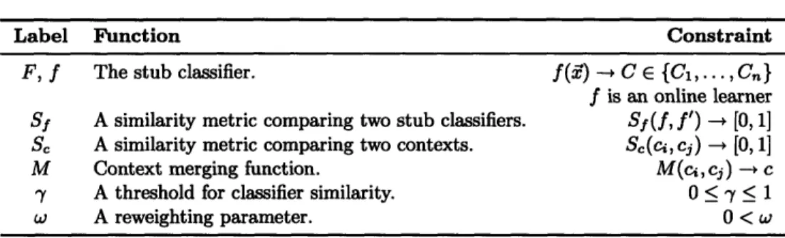
There are six parameters to the Context Dreaming algorithm: two num-bers defining a threshold and weight, and four functions for classification, comparison and context merging. These parameters are summarized in Ta-ble 3.1. How these parameters are used is explained in the sections below.
The stub classifier which Context Dreaming uses is the first parameter to the algorithm. This classifier must be an online (incremental) learner, and must support weighted learning, where some examples are more important than others. A simple way to add this weighting parameter to a classifier which doesn't have it is to repeat training examples multiple times. In this document, F will represent the class of classifier used as a stub, and f will represent an instance of this stub.
Context Dreaming requires two comparator functions, one for compar-ing contexts and one for comparcompar-ing classifiers. Both comparator functions return a similarity score ranging between zero and one, with zero being completely dissimilar, and one being a perfect match.
Another function required by Context Dreaming is M, which merges two contexts into a third.
Label Function Constraint
F, f The stub classifier. f (Y) - C E {C1,..., Cn}
f is an online learner Sf A similarity metric comparing two stub classifiers. Sy(f, f') - [0,1]
Sc A similarity metric comparing two contexts. Sc(ci, cj) [0,1]
M Context merging function. M(ci, cj) -, c
y A threshold for classifier similarity. 0 < 7 < 1
w A reweighting parameter. 0 < w
Table 3.1: Parameters to the Context Dreaming algorithm and their constraints.
Finally, two numeric parameters complete a Context Dreaming classi-fier. A number between zero and one serves as the threshold for classifier similarity (7). A weighting parameter, w, sets the adaptation rate during the wake phase.
Structure
A Context Dreaming classifier is a tuple (Sf, Sc, M, -y, w, L) where L is a set
of context and stub-classifier pairs, initialized to be empty. During oper-ation, the library is filled with context-classifier pairs, each context in the pair encapsulating the relevant components of the context which best match the paired classifier.
The data structure which describes situational contexts can come in many forms. The version implemented for this thesis is a key-value mapping, where the key is some symbolic label, and the value is a set of strings. In the phone-based troubleshooter example described above, one might choose the context keys such as "caller area code", "time of day", "weeks since product release" etc. For the color-naming experiment described in the next chapter, the context included the participant's native language, age, unique id, displayed image or word, etc. The relevance of any particular key is discovered by the algorithm.
W ake
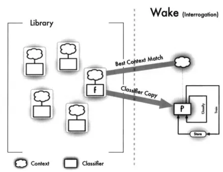
(Interrogation) IL - LIf~ LiBrary .... ...~. Context ( ClassifierFigure 3.1: Boxology of the Context Dreaming Wake cycle algorithm.
3.4
Phase
I
- The Wake Cycle
Each wake cycle covers an interrogation with constant context. The begin-ning of the interrogation is marked by submitting a context data structure to the classifier. This sets the internal state of Context Dreaming for the duration of the interrogation. After submitting the context, any number of classification or training requests can be made as long as the context remains fixed. At the close of the interrogation, a signal is sent to the Context Drea-ming classifier, ending the wake cycle. A single wake cycle corresponds to a single interrogation.
The submission of a context (c) to Context Dreaming primes the clas-sifier. First, Context Dreaming iterates over all the context-classifier pairs in its library L, comparing them to the incoming context using the context comparator Sc. The context receiving the highest score when compared to c is selected along with its accompanying classifier. Call this pair (cmax, fmax).
If the library is empty, then c is used as cax and the classifier prototype F is used as fmax,
Next, a copy of this maximum scoring classifier is made (f'nax) and set aside. The library L remains intact during the wake cycle. All classification and training examples submitted to Context Dreaming for the duration of the wake cycle are passed through fax. Training examples are submitted to
f'max with the weighting parameter w. They are also stored for replay during
the sleep cycle. It is by this means that a custom classifier is trained for the duration of the interrogation. In analogy to the hypothetical example, I learn what you mean by "democracy".
Algorithm 1 The Context Dreaming Wake Cycle Algorithm
On input (c):
if (L is empty) then
(cma., fma•) = (c, F)
else
(Cmaz, fm.a) = argmax (Sc(c, ci))
(c, Afi) EL
end if
f'nax copy(fmnax)
while (The interrogation is active) do if (Request is for a classification) then
Return the result of f4,,(I)
else if (Request is a training example (Ci, x)) then
Train f'na with (w, C, x)
Store example (Ci, x-)
end if end while
3.5 Phase
II
- The Sleep Cycle
At the end of an interrogative wake cycle, the Context Dreaming algorithm incorporates what it learned for future use. During this phase, the stub classifier fmax that was retrained over the course of the interrogation is in-corporated into the library. The integration happens in two steps. First, Context Dreaming uses the classifier comparator Sf to compare fmax (the retrained classifier used during the wake cycle) against all classifiers cur-rently in the library, L.
Sleep
(Integration)~LIVEUI
B
..
~..1
O
ClassifierFigure 3.2: Boxology of the Context Dreaming Sleep cycle algorithm.
Once the closest match is found, Context Dreaming completes the in-tegration. Consider the library classifier and associated context with the highest classifier similarity score s: (fi, ci)max. If the score s > -y then the training examples gathered during the wake cycle are "replayed" for fi, training fi using a weight of one. The two contexts ci (paired with the li-brary classifier) and cfI (paired with the interrogation's context) are merged together using M. This merged context is used as the new key for fi.
Otherwise, if s < -y then the
fmax,
and its associated context c, are added to the library.3.6
Expected Performance and the Effect of
Parame-ters
Making claims about the theoretical performance of a Context Dreaming classifier is difficult because of the wide flexibility of choosing a stub
classi-(38)
I:L ....
Algorithm 2 The Context Dreaming Sleep Cycle Algorithm
On input (cf , f.as) {Wake-cycle classifier flax and the interrogation context cf,}:
(fmatch,Cmatch) <-- argmax (Sf(fi, fM'na)) (fi,ci)EL
bestscore +- max (0, Sf(fmatch, fm/a)) if bestscore > 7 then
L.remove ((fmatch, Cmatch))
for Training example (C, x do
Train fmatch with (C, x- and weight 1
end for
cmerge +- M(c', Cmatch) L.add ((cmerge, fmatch))
else
L.add ((cI, f ar))
end if
fier, context data type, comparators, and the numeric parameters. Never-theless, some trends based on the effects of the parameters can be expected. As with other meta-classifiers, the performance of Context Dreaming is de-pendent on the performance of the stub classifier. We can expect that Con-text Dreaming will perform as well as the stub, but this is not guaranteed. In fact, if the y is set low, then no new stub classifier will be added to the
library--all training examples will be shunted to the prototype stub classi-fier F. Essentially, when y is very small, then Context Dreaming reduces to the stub classifier but with in-dialog fast adaptation. Over-fitting will result if y is set too high. In that case, the library will fill with contexts and classifiers that will be infrequently used.
The time-performance of Context Dreaming can be predicted as a func-tion of the performances of the parameter funcfunc-tions. The startup time of the wake cycle is O(ILI x O(Sc)) because of the single loop through each of the library's contexts. Any classifications and training during the wake cycle are O(fclassify) and O(ftrain) respectively: Context Dreaming merely passes the feature vector to the selected stub-classifier or adds a constant-time storage of training examples. Sleep-cycle constant-time performance is not much different: O (ILI x O(Sf) +m x (ftrain(4))) with m being the number of
training samples collected during the wake cycle. During this offline part, there is a single loop through the library, comparing classifiers, followed by
a training round looping once through the examples.
3.7 Algorithm Variants
The Context Dreaming algorithm provides fodder for a number of variants. Three are discussed here, the first of which may address some concerns about stability, the second scalability, and the third which can make more efficient use of the training data under certain assumptions of the data's form. Many other refinements to the algorithm can be imagined, whether conceptual or in implementation.
3.7.1 Hedging Your Bets
The Context Dreaming algorithm makes a hard guess by selecting a single stub classifier to take part in the wake cycle. If multiple contexts in the library receive the same top score when compared against the situation's context, there's no guarantee that the stub classifier Context Dreaming will choose will be correct. One way to soften this hard guess, and effectively have the meta-classifier hedge its bets is by choosing the top k context-classifier pairs from the library. These top k classifiers would vote to decide on a final classification for a feature vector Y. Voting could be weighted by each classifier's respective context-similarity score and classification confidence (if the stub classifier returns a confidence score.)
The sleep-cycle is also modified for this variant. Training examples gath-ered during dialog are reclassified by each of the k stubs and used to get a post-hoc evaluation of whether that classifier should have been included in the voting cohort. Those stubs which score above a threshold would be integrated into the library as described above. Those below would be discarded.
This modification should make Context Dreaming more robust and re-duce the variance of its classification error rate. The post-hoc assessment decreases the chances that a stub classifier in the library would be trained for a situation inappropriate for its context.
3.7.2 Refined Context Intersection
The Context Dreaming algorithm is agnostic to the description of context as long as the context comparator and intersection function match their respec-tive constraints. The version implemented to demonstrate Context Drea-ming operation though is limited by the context-merging and comparison functions-merging is accomplished by returning a context containing the intersection of the input contexts, and scoring is also based on amount of overlap. Therefore, merged context can only represent joint existence in the context ("ands"), with no way to represent alternatives ("ors"). The refined
context intersection described here is intended to overcome some of the first iteration's limitations.
The refined context is represented as a key-value histogram. Each value in the context is augmented with a count. Contexts are intersected by summing the counts in the values.
image: (grapes: 1) text : (eggplant: 2)
language: (english: 1) and language: (english: 2, japanese: 1)
are merged into
image: (grapes: 1)
language : (english : (1 + 2),japanese : 1) text: (eggplant : 2)
Using histograms for context values allows for better context similarity scoring. The context comparator function can produce a fuzzy notion of "and" as well as "or" using a relative entropy score such as the Kullback-Leibler divergence.
3.7.3 Training a Filter
This variant of Context Dreaming allows training examples to be applied to all contexts within the library and embraces Girdenfors' Conceptual Spaces [12]. To accomplish this, the Context Dreaming classifier is modi-fied, adding a parametric feature-transformer g(8, i) --+ ', where 0 are the parameters of the transform. Furthermore, the library of context and
stub-classifier pairs is replaced by a library of context and feature-transformer pairs. The wake and sleep cycles are changed as follows:
In the wake phase, the best matching context is chosen as described above. Any request for classification is first passed through the chosen feature-transformer, then classified by the stub classifier F. Fast adapta-tion for the duraadapta-tion of the wake phase comes by learning the parameter 0
(by hill climbing, simulated annealing or other such technique).
At the end of the interrogation, the newly trained feature transform is integrated into the library as is described above. Rather than a classifier comparator Sc, this variant uses a transform comparator So(Oi, Oj) -+ [0, 1] to score transform similarities. The y parameter now applies to this
similar-ity score. Any training examples gathered during the wake cycle are played back though g(0, ... ) and used to train the single stub classifier F.
3.8 Discussion
Comparing Context Dreaming to other machine learning algorithms can yield the following critique: How is Context Dreaming different from other mixed-data-type classifiers? Can't the contextual information be incorpo-rated into a single feature vector? Essentially:
x = 1xl, • •xn} where
context = {x1, ... , xi} and
Xfeatures = {xi+1,., Xn}
My response is to focus on the particulars of the use of a Context Dreaming classifier. Essentially, Context Dreaming should be considered within the
context of its use. Context Dreaming takes advantage of having a static
component (the context) and a dynamic one (i). The algorithm "locks in" on a particular stub classifier for the duration of an interaction: this fact allows for local adaptation to a particular interlocutor in a way that is not possible with a more general classifier. Furthermore, as a system, Con-text Dreaming is straightforward and flexible. It allows classifiers that use
only one data type (e.g. numeric values) to be augmented with mixed data types (e.g. symbolic contexts).
I conclude this chapter by summarizing the advantages of Context Drea-ming and the ways it takes advantage of the dialog model it works in.
* Context Dreaming allows for fast adaptation during a dialog with fixed context.
* The two phases of operation allow Context Dreaming to provide fast answers during an online dialog, and shunt more computationally ex-pensive procedures to the offline sleep cycle.
* Context Dreaming is well suited to interrogative tasks-situations which frequently arise in dialogues where there is a negotiation of the meanings of words.
* Classifiers accepting a single data type are transformed into mixed data type classifiers.
The next two chapters describe a color naming experiment and an evaluation of Context Dreaming on the corpus gathered.
CHAPTER
4
I
CONTEXT EFFECTS ON COLOR NAMING
The words we use to label colors in the world are fluid. They are dependent on lighting conditions, on the item being named, and on our surroundings. The color stimulus you might label as "orange" in one context, you would label "red" when talking about hair. Likewise, "black" becomes "red" when talking about wine. The grass would still be called green when lit by a red-tinted sunset. Although we intuitively know this context effect exists, I wish to quantify it under controlled circumstances.
This chapter describes an experiment I designed in part to gather a cor-pus on which to evaluate the Context Dreaming algorithm. The experiment was built upon a particular color negotiation task described previously. A colleague sitting across a table asks you to "pass the blue one." To your eyes though, there's only a cyan object and a purple one. Which do you choose? The experiment described here distills this task to its most primi-tive components. Further discussion of the way the experiment encodes this hypothetical scenario can be found in the next chapter, which describes the application of the corpus on a Context Dreaming classifier.
The results of the experiment confirm that semantic context affects color categorization, although sometimes in surprising ways. The first part of this chapter describes the experiment performed, and the second discusses the
sex # Min age Max age Mean age Male 8 18 45 26.6 Female 15 18 63 43.3 Native language # English 18 Chinese 3 Portuguese 1 Spanish 1
Table 4.1: Demographics of the study participants.
results and proposes a model which may account for the data.
4.1
Experiment
I designed an experiment to validate the hypothesis that situational and se-mantic context affect the naming of colors. The experiment consists of three color-related tasks: calibration, forced choice and naming. The calibration task provides a baseline on which to evaluate the naming and forced choice tasks. Both naming and forced choice parts evaluate contextual effects on color categorization by presenting an ambiguous color stimulus and forcing the experimental subject to make a categorical decision.
To prepare stimuli to be presented in this experiment, a separate stimulus-selection data collection was run.
4.1.1 Participants
Thirty-six participants were solicited from the MIT community by email an-nouncements and posters. Inclusion criteria was proficiency with the English language. Participants were asked to provide their age, sex, native language and any other languages they spoke fluently. Participants were compensated for their time. From these, the first 13 were chosen to complete only the stimulus-selection task.
4.1.2 Equipment
The experiment was performed in a windowless, dimly lit room illuminated at approximately 32000K. Approximately ten minutes were spent adjusting