Cost-benefit analysis of ultra-low sulfur jet fuel

Cost-benefit Analysis of Ultra-Low Sulfur Jet Fuel

by

Stephen Kuhn

B.S. in Mechanical Engineering, Carnegie Mellon University, 2008

Submitted to the Department of Aeronautics and Astronautics

in Partial Fulfillment of the Requirements for the Degree of

Master of Science in Aeronautics and Astronautics

at the

MASSACHUSETTS INSTITUTE OF TECHNOLOGY

ARCHNES

May 2010

May201

© Massachusetts Institute of Technology 2010.

JUN

2 3

2010

All rights reserved.

LIBRARIES

A u th o r... ... ...

"i"epart nent of Aeronauhcs and Astronautics lay 24, 2010

Certified by...

Ian A. Waitz

Jerome C. Hunsaker Professor of Aeron cs and Astronautics Department Head

Thesis Supervisor

Accepted by...

David L. Dar oI

Professor of Aeronautics and Astronautics Associate Department Head Chair, Committee on Graduate Students

Cost-benefit Analysis of Ultra-Low Sulfur Jet Fuel

by Stephen Kuhn

B.S. in Mechanical Engineering, Carnegie Mellon University, 2008

Submitted to the Department of Aeronautics and Astronautics in Partial Fulfillment of the Requirements for the Degree of

Master of Science in Aeronautics and Astronautics

Abstract

The growth of aviation has spurred increased study of its environmental impacts and the possible mitigation thereof. One emissions reduction option is the introduction of an Ultra Low Sulfur

(ULS)

The cost of a ULS jet fuel policy is well-characterized by the adoption of ULS diesel fuel, similar to jet fuel, for ground transportation in the US and elsewhere. The cost of hydrodesulfurization

(HDS), the process used to remove sulfur from fuel, is projected to be between 4 and 7 cents per gallon of jet fuel. With 2006 levels of domestic fuel consumption, this translates to a yearly cost of HDS of $540-$940 million within the US. The climate and air quality benefits are characterized by several earth-atmosphere models, which isolate the perturbation of aviation emissions. Comparisons among models, which employ different modeling methods and assumptions as well as different spatial resolution, provide some cross-validation, as well as characterizing the degree of uncertainty in the state of the science. This thesis focuses in detail on the CMAQ (Community Multi-scale Air Quality) model, used by the Environmental Protection Agency (EPA) to support regulatory impact assessment. Other models, their results, and efforts at inter-model comparison are also discussed. Benefits are monetized through valuing the reduction in premature mortality from reduced concentrations of ground-level particulate matter (PM).

The central finding from CMAQ is that with nominal health impact parameters, a global ULS jet fuel policy is predicted to save 110 lives per year in the US when considering full flight emissions, a 14% reduction in aviation-attributable mortality resulting in an estimated monetary benefit of $800 million.

Acknowledgments

During the work entailed in this thesis, I received support and assistance from many people, some of whom I would like to thank here.

My advisor Ian Waitz has been instrumental in guiding the course of the ULS project in the face of setbacks and over the course of much spirited debate. He has been a pleasure to work for, and I've learned a great deal from him. His style is well-suited to bringing out the best in the people he works with. Special thanks as well to Steven Barrett, whose knowledge of atmospheric chemistry and tools has been invaluable, and whose assistance and time has been generously gifted.

Thanks to my friends and colleagues in the PARTNER lab, with whom I have discussed much. Thanks to Tudor Masek, who helped answer many questions well after he had left us; Elza Brunelle-Yeung, who brightened the windowless and decrepit expanse of my first office, and helped in many other ways besides; Akshay Ashok, to whom I gladly yield the mantle of pseudo-computer expert; Pearl Donohoo, who suffered mightily, and lived to fight another day; Rhea Liem, whose behaviors can only be described as stochastic; Jim Hileman, a project and lab leader who has helped guide many students' work; Russ Stratton and Matthew Pearlson, who along with Jim and Pearl researched and compiled the cost part of the study; and all the rest I knew and worked with.

Thanks as well to the scientists and engineers at UNC, FAA, EPA, Cambridge, Harvard, Stanford, and elsewhere who helped to make, run, and interpret the models used in the study. There were many labors and countless emails; I appreciate the time and effort put in by all.

I would also like to thank the MIT Aeronautics and Astronautics Department for helping to make my time at MIT interesting.

Table of Contents

Abstract...3

Acknowledgm ents...

4

Table of Contents ...

5

List of Figures ...

8

List of Tables...

11

List of Sym bols ...

12

1

Introduction...14

2

Setup ...

15

2.2.2.1 AEDT/SAGE, FOA3 and Emissions Indices ... 21

2.2.2.2 NOx by Flight Mode...22

2 .2 .2 .3 L igh tn ing N O x ... 24

2.2.2.4 H ydrocarbon Split... 27

2.2.3 Processing Methodology ... 28

2.3 Background Inventories... 28

2 .3 .1 B ackgro u n d ... 2 8 2.3.2 Species Population from National Emissions Inventory...29

2.3.2.1 2001 N E I vs. 2005 N E I... ... 29

2.3.2.2 Surface C oncentrations ... . ... 29

2.3.2.3 V ertical profiles ... 30

2.4 GEOS-Chem Boundary Conditions ... 34

2 .4 .1 B ackgro u n d ... 34

2.4.2 GEOS2CMAQ and methodology ... 34

2 .4 .3 V erificatio n ... 3 5 2.5 Meteorological Data...38

2 .5 .2 V ertical P ro files...40

2.6 Particle-Bound W ater and Dry vs. W et PM ... 40

2.7 Population Data and H ealth Impacts...42

2.7.1 Global Population of the World (GPW) and Global Rural-Urban Mapping Project (G R U M P ) ... 4 2 2.7.2 Concentration Response Functions... ... 43

2.7.3 Monetary Value of a Statistical Life (VSL)... ... 46

2.8 M odeling Context ... 46

2.8.1 Earth-Atmosphere Modeling of Aviation... 46

2.8.2 Atmospheric Aerosols ... 47

2.8.3 Multi-Model Approach... 50

3

Full Flight Emissions Assessment...

52

3.1 Context ... 52

3.2 Changes in Surface Concentration and M ortalities...52

4

L TO Em issions Assessm ent...57

4.1 Context ... 57

4.2 Changes in Surface Concentration and M ortalities...57

5

Clim ate Feedbacks...

62

5.1 Background on Climate Feedbacks... 62

5.2 Background on GATOR-GCM OM ... 62

5.3 Future W ork ... 64

6

ULS Cost and Operations Analysis ...

64

6.1 Sulfur Content of ULS Jet Fuel...64

6.2 Production Costs of ULS Jet Fuel...66

6 .2 .1 B ack gro u n d ... 6 6 6.2.2 Detailed Cost Analysis ... 67

6.2.2.1 Normalized Crack Spread of Diesel and Jet Fuels ... 69

6.2.2.2 Supply and Demand ... 69

6.2.2.3 The Cost of a Gallon of Diesel... 69

6.2.2.4 Historic Price Difference in Diesel Fuels ... 70

6.2.2.5 Processing Costs... 70

6.2.2.6 Limitations of this Analysis ... 70

6.2.3 Production Cost Estimate ... 71

6.3 Potential Usability Concerns and Benefits with ULS Jet Fuel... 71

7

CM A Q Sensitvity Studies...

74

7.1 CM AQ models ... 74

7.3 Vertical Diffusion and Advection... 76

7 .3 .1 B ackgro u n d ... 76

7.3.2 Vertical Diffusion: EDDY vs. ACM 2... ... 77

7.3.3 Vertical Advection: PPM vs. YAM O ... 78

7.4 Static vs. Changing Background Conditions... 79

7 .4 .1 C o n tex t...7 9 7.4.2 Dominance of GEOS-Chem Boundary Conditions ... 79

7.5 Lightning N Ox ... 80

8

Com

parisons to Em pirical

D ata ...

83

8.1 Context ... 83

8.2 Speciated M odel Attainm ent Test ... 83

8 .2 .1 M eth o d o lo gy ... 83

8 .2 .2 R e su lts ... 8 4 8.2.3 EPA FRM monitor sites...86

8.2.4 Comparisons of Outputs to M onitor Data... 86

9

Lim itations and Future W ork ...

89

9.1 Scope/Feedback ... 89

9.2 Uncertainty...90

9.3 Other Differences...90

9.4 UT/LS Transport in CM AQ ... 91

9.5 Proposed Paths Forward...92

10

Conclusion...94

10.1 CTM Findings...94

10.2 Cost/Benefit Assessm ent... 94

A PPEN

D ICE

S...

95

Appendix A: CMA Q Inventory and Model Species ...

95

A.1 Aircraft Em issions Inventory ... 95

A.2 Background Inventory and Concentrations ... 102

A.3 CM AQ Outputs... 106

Appendix B: CM A Q Processes ...

108

B.1 Carbon-Bond IV Processes and Reactions M odeled ... 108

Appendix C : CM A

Q

R esults ...

113

A.1 Additional Aviation Results ... 113

A.2 Computational Tim e/Complexity...117

List of Figures

Figure 1: CMAQ horizontal domain used in the ULS study (Masek, 2008)...18

Figure 2: CMAQ vertical structure (CMAQ 4.6 Operational Guidance Document, 2009) ... 19

Figure 3: Emission indices of NO, N02, and HONO from a CFM56-3B1 engine (Wood, Herndon, Tim ko, Y elvington, & M iake-Lye, 2008)... 23

Figure 4: Vertical Profile of N from Lightning NO over the CMAQ US domain ... 25

Figure 5: Vertical columnar sum of N [g N/yr] from lightning emissions of NO for 2006 ... 26

Figure 6: NASA NSSTC space-based observation of #flashes/km^2/yr., 1995-2000 (Where L ig h tn in g S trik es) ... 2 6 Figure 7: 2006 background NH3 and PM2.5 concentration showing several co-located hotspots ....30

Figure 8: Comparison of 2001 and 2005 NEI emissions profiles over CMAQ US domain...31

Figure 9: NEI emissions trends of several key species (National Emissions Inventory Air Pollutant T ren d s D ata, 2 0 0 9) ... 32

Figure 10: Seasonal Variability in the 2001 NEI for several key emissions species ... 33

Figure 11: Ground level 03 concentrations [ppbV] from GEOS-Chem (inside the black box) and the CMAQ BCON created from this GEOS-Chem run (outside the black box) ... ... 36

Figure 12: Ground level 03 concentrations in a.), and at ~860hPa (layer 10) in b.); ground level HNO3 concentrations in c.), and at ~860hPa in d.) ... 37

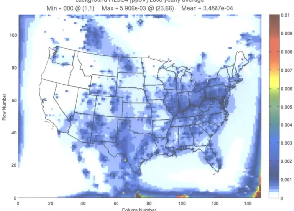
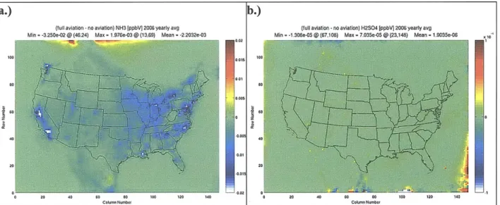
Figure 13: Background H2SO4 showing higher concentrations at domain boundary at ground level ... 3 7 Figure 14: Full aviation delta in ground-level NH3 and H2SO4, showing clear boundary layer effects ... 3 8 Figure 15: Vertical profiles of US average temperature, cloud water mixing ratio, rain water mixing ratio, and w ater vapor m ixing ratio ... 40

Figure 17: CM A Q dom ain population... 43

Figure 18: Health impact pathway for air quality assessment (Rojo, 2007)...43

Figure 19: Baseline cardiopulmonary and lung cancer mortalities ... 45

Figure 20: Spatial and temporal scale of atmospheric processes (Seinfeld & Pandis, 2006) ... 47

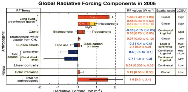
Figure 21: Global Radiative Forcing from All Anthropogenic Sources of Emissions (Lee, et al., 2 0 0 9 ) ... 4 9 Figure 22: Global Radiative Forcing from Aviation Emissions (Lee, et al., 2009) ... 50

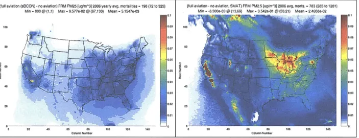
Figure 23: Full aviation FRM PM2.5 and ULS reduction in same, full aviation (static BCON) FRM

PM 2.5, and post-SM A T FR M PM 2.5...54

Figure 24: Full aviation S04, N03, and NH4, and ULS reduction in same ... 55

Figure 25: Full aviation BC and ORG, and ULS reduction in same ... 56

Figure 26: Speciated components of full aviation-attributable change in FRM PM2.5 and mortalities ... 5 6 Figure 27: Speciated components of ULS aviation-attributable change in FRM PM2.5 and mortalities ... 5 7 Figure 28: LTO aviation FRM PM2.5 and ULS LTO reduction in same, LTO aviation (static BCON) FRM PM2.5, post-SMAT FRM PM2.5...58

Figure 29: LTO aviation S04, N03, NH4, and ULS reduction in same...59

Figure 30: LTO aviation BC and ORG, and ULS reduction in same...60

Figure 31: Speciated components of LTO aviation-attributable change in FRM PM2.5 and m o rtalitie s ... 6 1 Figure 32: Speciated components of ULS LTO aviation-attributable change in FRM PM2.5 and m o rtalitie s ... 6 1 Figure 33: Jet A average fuel sulfur content in US (Taylor, Feb. 2009), as plotted by (Hileman, et al., 2 0 0 9 ) ... 6 5 Figure 34: JP-8 fuel sulfur content as reported by PQI (DESC-BP, 1999-2007), as plotted by (H ilem an , et al., 2 0 09) ... 6 6 Figure 35: Jet A-1 average fuel sulfur content in UK (Rickard, June 2008), as plotted by (Hileman, et al., 2 0 0 9 ) ... 6 6 Figure 36: D iesel prices and production... 68

Figure 37: Sensitivity of results to vertical diffusion parameter ... 78

Figure 38: Dominance of GEOS-Chem boundary conditions ... 79

Figure 39: Sensitivity of results to LN O x... 82

Figure 40: Full aviation post-SMAT speciated results in comparison to pre-SMAT model outputs.. 85

Figure 41: Full aviation SMAT constituent contribution to FRM PM2.5 in comparison to pre-SMAT m o d el o u tp u ts...8 5 Figure 42: EPA FRM monitor sites used in SMAT software (Abt Associates, Inc., 2009)...86

Figure 43: Comparison of CMAQ monthly average ground-level FRM-hydrated PM2.5 to quarterly (native) official FRM monitor data... ... ... 88

Figure 44: Comparison of monthly average ground-level FRM-hydrated PM across models to

quarterly (native) official FRM m onitor data... 89

Figure 45: APMT-AQ projections of changes in FRM PM2.5 (a.) and b.)) in comparison to LTO-only (static B C O N ) results from C M A Q ... 91

Figure 46: AEDT vertical profiles of US yearly aircraft emissions ... 97

Figure 47: CMAQ processed input vertical profiles of US yearly total aircraft emissions...99

Figure 48: CMAQ processed input vertical profiles of US yearly total aircraft emissions (continued) ... 1 0 0 Figure 49: CMAQ 2006 yearly average background species concentrations ... 106

Figure 50: Hierarchical relationship between major species in CB-IV (Isukapalli, 1999)... 109

Figure 51: Full aviation-attributable changes in precursor and oxidizing gases ... 115

List of Tables

Table 1: Scenarios included in the design of experiment... 17

Table 2: CMAQ sigma layers used for ULS, with sea-level referent corresponding pressures/altitudes ... 2 0 T ab le 3: E m ission s in dices...22

Table 4: Calculation of total N02 and NOx emissions from a CFM56-3B1 during LTO cycle (Wood, Herndon, Timko, Yelvington, & Miake-Lye, 2008) ... 24

Table 5: Speciated split of NOx into CMAQ species...24

Table 6: Hydrocarbon split into CB-IV species ... 28

Table 7: GEOS-Chem to CMAQ species mapping (Moon, Park, Li, & Byun, 2008)...34

Table 8: CMAQ/MM5 meteorological parameters and mechanisms... 39

Table 9:

P

Table 10: Summary Model Comparison...51

Table 11: Refining and crude oil costs of a wholesale gallon of diesel, May 2002 -August 2009 (Spot P ric e s, 2 0 1 0) ... 6 9 T able 12: C M A Q schem es/m odels...74

Table 13: ULS CMAQ "baseline" options (CMAQ 4.6 Operational Guidance Document, 2009)...75

Table 14: Sensitivity studies scenarios proposed...76

T able 15: P roposed future w ork ... 92

Table 17: Full aviation total aircraft emissions from AEDT...95

Table 18: Full aviation total aircraft emissions CMAQ processed input totals ... 98

Table 19: Corresponding molecular weights for HC species and groupings in Table 18 i.e. (MF/SF) ... 9 8 Table 20: Aircraft emissions pre-processed, speciated hydrocarbon profile (FAA OEE & EPA O T A

Q

Table 22: CMAQ4.6 concentration output species and descriptions (Isukapalli, 1999) ... 106

List of Symbols

AEDT -Aviation Environmental Design Tool

APMT -Aviation Portfolio Management Tool

AQ - Air Quality

AQM - Air Quality Model

BC - Black Carbon (soot)

BCON - Boundary Conditions

CAEP -Committee on Aviation Environmental Protection

CBIV - Carbon Bond IV (4) CBV - Carbon Bond V (5)

CCN - Cloud Condensation Nuclei CH4 - Methane

CI - Confidence Interval

CMAQ - Community Multi-scale Air Quality Model

CRC -Coordinating Research Council

CRF -Concentration Response Function

CTM - Chemistry and Transport Model

EC - Elemental Carbon (soot, also called BC)

El -Emissions Index

EIA -Energy Information Agency

EPA -Environmental Protection Agency

EPAct - Energy Policy Act

FAA - Federal Aviation Administration

FOA3 -First Order Approximation Version 3.0

FRM -Federal Reference Method FSC -Fuel Sulfur Content

GATOR-GCMOM - Gas, Aerosol, TranspOrt, Radiation, General Circulation, Mesoscale, Ocean

Model

GCM - Global Climate Model

GHG - Greenhouse Gas

GEOS -Goddard Earth Observing System

HC -Hydrocarbon

HDS -Hydrodesulfurization

HOx -OH and applied radicals

HSD -High-Sulfur Diesel

ICAO - International Civil Aviation Organization

ISORROPIA - CMAQ inorganic gas-aerosol equilibrium model, from the Greek for "equilibrium"

IMPROVE -Interagency Monitoring of PROtected Visual Environments

IPCC -Intergovernmental Panel on Climate Change

LOSU - Level of Scientific Understanding

LS - Lower Stratosphere LSD -Low-Sulfur Diesel

LTO - Landing and Takeoff Cycle (<1 000m AGL)

MM5 -Mesoscale Model Version 5 NEI -National Emissions Inventory NH3 -Ammonia

NH4 -Ammonium ion

N03 - Nitrate ion

NOx - Nitrogen Oxides (NO + N02)

03 -Ozone

OH -Hydroxyl radical ORG - Organics

PBL -Planetary Boundary Layer PM -Particulate Matter

PM2.5 - Particulate Matter smaller than 2.5 micrometers in diameter (as nearly all

aviation-attributable aerosols are)

PMFO -Primary Fuel Organics PMSO -Primary Sulfur Organics

nvPM - non-volatile Particulate Matter

PBL -Planetary Boundary Layer

ppbV - parts per billion Volumetric

ppm -parts per million

RF - Radiative Forcing RH - Relative Humidity

SAGE -System for assessing Aviation's Global Emissions

SANDWICH - Sulfate, Adjusted Nitrate, Derived Water, Inferred Carbonaceous mass Hybrid

material balance

SMAT -Speciated Model Attainment Test

S04 -Sulfate ion

SOx - Sulfur Oxides

STN - Speciation Trends Network SULF -Sulfuric Acid (H2SO4) THC - Total Hydrocarbon TOG - Total Organic Gases

ug/m^3 - micrograms per meter cubed ULS -Ultra Low Sulfur

ULSD - Ultra Low Sulfur Diesel ULSJ -Ultra Low Sulfur Jet

1

Introduction

1.1

Context

Global aviation has historically been a fast-growing industry. Its rate of growth has outstripped the growth of gross domestic product by a factor of 2.4 between 1960 and 1999 (IPCC, 1999), and despite a lull in the past decade due to terrorist attacks and economic downturn, steady growth is projected into the future. Concerns related to the noise, climate, and air quality impacts of aviation are increasingly voiced.

On a global scale, aircraft emissions of greenhouse gases (GHGs) and precursors contribute to climate change (IPCC, 1999). On a regional scale, aircraft emissions impact air quality, with resulting health impacts (ICAO, 2007). Poor air quality has been linked to premature mortality (US EPA, 2006), cardiovascular and pulmonary hospital admissions, and asthma aggravation (US EPA, 2004), among other ailments.

Aviation is largely unique among the anthropogenic sources of emissions in that its emissions extend well into the atmosphere, to the free troposphere and jet stream, and even into the lower stratosphere, resulting in impacts that can be felt over a larger distance and longer time than ground-based emissions sources. Long-lived species (compounds) and precursors can be transported across oceans and continents.

1.2

Motivation

Reductions in aircraft emissions per flight can be effected in one of three ways; changes in operational procedures for greater efficiency; changes in aircraft technology; and changes in fuel composition. Operational changes have been the subject of much research and development, and are embodied in the systems used to route and manage commercial aviation. Such systems are developed at great cost over many years, and often require the development of new technology, including the installation of new avionics equipment in aircraft. Airframe and engine improvements are likewise emphasized in improving fuel efficiency and performance, but a given airframe and engine are typically used in the fleet for 30 or more years (Morrell & Dray, 2009), and new technology takes many years to develop. _{Furthermore, retrofitting existing aircraft is typically} prohibitively expensive. Therefore changes in operational procedures and aircraft technology are felt only gradually, over decades. In contrast, changes in fuel composition result in immediate changes in emissions. In the case of ULS fuels, which are assumed in this study to contain 15ppm sulfur, the technology and infrastructure for HDS exists from the EPA-mandated conversion of diesel to ULS diesel for most types of US ground transportation. The adoption of ULS diesel has phased into effect since 2006 (US EPA, 2006) (US EPA, 2006) and entails an identical chemical process. Projected costs, and especially capital expenditures, are much less speculative for the adoption of ULS jet fuel than for most other emissions mitigation options for aviation.

The precursor gases NOx and SOx are the two largest sources of aviation-attributable ground level particulate matter (PM). The species oxidize ammonia (NH3) existing in the atmosphere from non-aviation sources to form sulfates and nitrates. Other sources of non-aviation-attributable PM include soot (black carbon, or BC), largely dependent on aromatic and paraffmic fuel content, and organic compounds, which typically account for less than 5-10% of aviation-attributable PM in this and prior studies (Rojo, 2007), (Masek, 2008). NOx is created in the aircraft engine combustor as a

byproduct of the combustion of air (~78% N2) and fuel at high temperature. Its emission is

dictated entirely by the processes within the combustor. As such, NOx reduction is dependent on the implementation of new engine technology in the fleet. SOx is created during combustion as sulfur in the fuel is oxidized. It is therefore possible to completely control SOx emissions by changing fuel composition.

1.3

Contributions

This thesis presents some results from the study of a switch to ULS jet fuel. It addresses original work from several parties, which is labeled as such where applicable. Four earth-atmosphere models were used to predict the climate and air quality benefits of a ULS jet fuel policy. These include GATOR-GCMOM (Gas, Aerosol, TranspOrt, Radiation, General Circulation, Mesoscale, Ocean Model), GEOS-Chem (Goddard Earth Observing System Chemistry Model), TOMCAT, and

CMAQ (Community Multi-scale Air-Quality Model). This thesis describes some results from

several of these models, but focuses primarily on the CMAQ model. The setup, inputs, and outputs of the CMAQ model are described in detail. The mining and integration of data, where results from different models are compared together, are original to this thesis.

1.4

Thesis Structure

This thesis is organized into 11 sections. Introduction and setup of the model runs are followed by results from full-flight and landing-takeoff (LTO)-only emissions scenarios. A general discussion of results when climate feedbacks are modeled is included. Afterwards follows analysis of sensitivities

to various parameters in CMAQ, as well as comparisons of model data to empirical data. Then

limitations, future work, and conclusions are presented.

2

Setup

2.1

CMAQ

2.1.1

Background

The EPA's Community Multiscale Air Quality (CMAQ) model is a three-dimensional Eulerian atmospheric chemistry and transport modeling system that simulates ozone, acid deposition, visibility, and fine particulate matter throughout the troposphere (CMAQ 4.6 Operational Guidance

Document, 2009). Like all Eulerian computational air quality models, on a fundamental level, CMAQ outputs concentration fields that are the solutions of systems of partial differential equations for the time-rate of change in species concentrations due to a series of individual physical and chemical processes, which are aggregated. Air quality models integrate our understandings of the complex processes that affect the concentrations of pollutants in the atmosphere. Establishing the relationships among meteorology, chemical transformations, emissions, and removal processes in the context of atmospheric pollutants is the fundamental goal of such a model (Seinfeld & Pandis, 2006). CMAQ uses a set of modular process solvers to accomplish this, which incorporate models developed in the literature (Table 12 in Section 7).

2.1.2

Model Scenarios

The procedure for studying a particular phenomenon or perturbation, such as the effect of aircraft emissions on ground-level PM and ozone, is as follows. A scenario is run (Run 1) in which every source of emission - biogenic and anthropogenic, industrial, transportation, etc. - is included, except the perturbation. This is the so-called "background" inventory and is compiled from the EPA's National Emissions Inventory (NEI) for the US, and from various sources for the rest of the world. An inventory is a gridded or spatial accounting of emissions rates (i.e. in g/s or mol/s, depending on the phase of the species, using accounting of hourly changing emissions profiles). In this case, the background omits any aviation emissions. The model is run for a given amount of time, processes evolve, and concentrations are saved (i.e. in ug/m^3 or ppbV, depending on the phase of the species). Another scenario is run in which the perturbation inventory, in this case the aircraft emissions inventory, is added to the background inventory (Run 2). The interactions of the aircraft emissions with background species and emissions, including NH3, 03, OH, and S02, among others, are captured. The model is run, and concentrations are saved. Run 1 is subtracted from Run 2, and the impacts of aviation emissions within the wider atmospheric system are isolated. For aviation, this difference, or "delta" case change in concentration, is typically a small fraction of the absolute, or ambient, concentrations (the output of Run 2); depending on location, for all species of PM, aviation-attributable concentrations are at least two orders of magnitude lower than ambient, and often much lower still. Some representative plots of this relative contribution are provided in Appendix C.

In addition to the background, there are four aviation scenarios for the ULS project, listed in Table 1. All models used in the study scoped these scenarios at the least, though domains and durations varied, and additional variations were added for different models. The full aviation, or "baseline", scenario represents full flight emissions with current fuel compositions. Fuel compositions are discussed in detail in Section 6.1. The ULS full aviation scenario represents full flight emissions with a ULS fuel composition. Until recently, it was thought that LTO (landing and takeoff, <1km above ground level) emissions contributed to the bulk of ground-level PM. However, that has been called into question by (Barrett, Britter, & Waitz, 2009) and the finding that cruise emissions may contribute between two and 10 times the amount of ground-level PM as LTO emissions, as predicted by GEOS-Chem. A secondary objective of this study is to further examine the relative

impact of cruise emissions. As such, scenarios were included in which LTO-only aircraft emissions were modeled, as well as LTO-only emissions with a ULS fuel policy. These also provide valuable comparisons to previous LTO-only studies.

A three-month "spin-up" was included for each scenario. This provides sufficient time for

concentration gradients and transport processes to develop before the period of study. For CMAQ,

that period is the full year of 2006. All aviation inventories for the project, as well as the

meteorological data for CMAQ and GEOS-Chem are from 2006. The background inventory is notably based on the 2001 NEI. Over the US, GATOR-GCMOM uses the 2005 NEI, and GEOS-Chem uses the 1999 NEI. A comparison of the 2001 and 2005 NEIs is provided in Section 2.3.2 for several CMAQ species. It was impractical to harmonize the NEI years across models due to general availability at the time, but the differences between models are far more significant than the differences between the background inventories.

The boundary conditions (BCON) for CMAQ (the "picture frame" concentrations at the edge of the domain) were derived from global GEOS-Chem runs in which the scenario was also allowed to

change. For instance, the inventory for the global GEOS-Chem run that was used for the

background scenario CMAQ BCON also included no aviation emissions. Two additional scenarios beyond the design of experiment were included for CMAQ in which the full aviation and LTO scenarios used static BCON; that is to say, the background BCON were used for these scenarios, eliminating differences in BCON flux in the delta case, and isolating the component of change over the US that is due to US-only changes in aircraft emissions.

Table 1: Scenarios included in the design of experiment

Background

Spin-up (Oct-Nov 2005), Scenario Gan-Dec 2006)

Full aviation, or "baseline" _{Spin-up (Oct-Nov 2005), Scenario Gan-Dec 2006)}

ULS full aviation _{Spin-up (Oct-Nov 2005), Scenario Gan-Dec 2006)}

LTO aviation

_{Spin-up (Oct-Nov 2005), Scenario (Jan-Dec 2006)}

ULS LTO aviation

Spin-up (Oct-Nov 2005), Scenario Gan-Dec 2006)

2.1.3

Model Domain

The CMAQ grid is a Lambert conformal conic projection covering the continental United States and parts of Canada, Mexico, and the Caribbean. The 3-D grid is of size 148 x 112 x 35, constituted of 148 cells from western to eastern boundaries, and 112 grid cells from northern to southern, of 36 x 36km within the projection, extending upwards into 35 vertical layers. The domain boundary is not rectilinear in latitude/longitude coordinates, so e.g. the western border spans a range of longitudes. This can be visualized in the CMAQ plots in Section 8. The vertical layers are finer at ground level and become coarser as they ascend, with eight layers in the lowest km and an upper limit of 1OOhPa (-15-17km). The parameters of the Lambert projection, including the standard parallels, central meridian, and latitude of origin, are shown in Figure 1. Lambert conformal

projections minimize two-dimensional distortion of the three-dimensional portion of the Earth's surface over the US domain, with zero distortion along the standard parallels, at 33N and 45N. Lambert projections are also favored in general for aviation because a straight line drawn on the projection approximates the great-circle route between endpoints that aircraft generally attempt.

Figure 1: CMAQ horizontal domain used in the ULS study (Masek, 2008)

The CMAQ vertical domain is a non-hydrostatic sigma coordinate system, described by a set of dimensionless parameters, denoted sigmas by convention, defined in Equation 1.

= P-Prop

* Pgroundref' Prop

Each vertical column has a layer structure that is normalized to the difference between the reference pressure at mean ground-level and 1OOhPa. In essence, this allows the vertical coordinate system to be terrain following. The sigmas (which have values between 1, at ground level, and 0, at 1OOhPa) are then used to determine the pressure at the edges of each vertical layer. As each of the 148 x 112 vertical columns have the same number of layers, and yet different mean ground altitudes (and

therefore pressures), each vertical column has a unique grid. This can be visualized in Figure 2. The sigmas themselves are based on the lowest levels of the existing CMAQ 2001 NEI used in prior studies, as well as the reduced vertical domain of GEOS-5 (Goddard Earth Observing System Model-5) for general boundary condition compatibility. For the purposes of displaying the results of this study, the vertical grid normalized to sea level was taken as the referent for plots of

domain-average concentration by pressure. This results in a uniform aggregation of all surface layer

concentrations into the same vertical bin, which would otherwise not be the case. A more rigorous method would require paired-in-time-and-space summation, which is prohibitively intensive for the quantity of data generated, and which would conflict with the method of display of other models in the study (which also use sigma, as opposed to eta or hybrid sigma-eta coordinates, in which the ground layer varies).

Pr =const

=~~~hx

p'X(

h

=/-c

)X _MSL

Figure 2: CMAQ vertical structure (CMAQ 4.6 Operational Guidance Document, 2009)

The sigma layers in Table 2 are used to create the pressures at top and bottom of a vertical grid cell. For example, the bottom of layer 1 is described by the sigma 1.000, and the top by 0.9950. The bottom of layer 2 is described by 0.9950, and the top by 0.9900, etc. The pressure and altitude for a vertical column normalized to sea level are also listed, where the pressure and altitude describe the top of the layer. These pressures and altitudes vary, however, with the ground altitude for a given vertical column.

Table 2: CMAQ sigma layers used for ULS, with sea-level referent corresponding pressures/altitudes 1 (ground layer) 1.0000 1013.5 0.6377 682.59 3,260 2 0.9950 1008.9 20.1 20 0.5959 644.35 3,652 3 0.9900 1004.4 60.3 21 0.5541 606.17 4,144 4 0.9800 995.23 121.0 22 0.5123 567.99 4,662 5 0.9600 976.96 243.4 23 0.4706 529.89 5,208 6 0.9400 958.69 408.9 24 0.4288 491.71 5,787 7 0.9100 931.29 619.6 25 0.3871 453.62 6,404 8 0.8830 906.62 865.1 26 0.3453 415.53 7,063 9 0.8663 891.37 1,057 27 0.3036 377.34 7,772 10 0.8495 876.02 1,207 28 0.2619 339.25 8,539 11 0.8328 860.76 1,359 29 0.2071 289.19 9,516 12 0.8161 845.50 1,513 30 0.1593 245.52 10,686 13 0.7993 830.16 1,670 31 0.1187 208.43 11,837 14 0.7770 809.79 1,856 32 0.0844 177.10 12,951 15 0.7492 784.39 2,099 33 0.0553 150.52 14,025 16 0.7213 758.91 2,377 34 0.0305 127.86 15,065 17 0.6934 733.42 2,663 35 0.0095 108.68 16,070 18 0.6656 708.03 2,957 0.0000 100.00 16,819 The comprehensive diffusion, advection, set of aerosol CMAQ module,

settings used for such parameters as chemical mechanism, etc. are described in more detail in Table 13 in Section 7, the section on CMAQ sensitivity to changes in those parameters.

2.2

Aviation Inventories

2.2.1 Introduction

Aviation emissions inventories convert flight data into rates of species emission, using information about the flight mode (i.e. throttle level and altitude), engine and airframe type, fuel type, and temperature, pressure and other environmental conditions. Chord-level flight data is scaled based on relations governed by these parameters, and aggregated to the grid structure. Aviation-attributable PM is grouped into two categories: primary PM and secondary PM created from aviation-attributable precursors. Primary PM is created in the combustor and turbine itself; at the

plane of the exit nozzle, the species are extant. Secondary emissions are formed in the plume of the engine exhaust and elsewhere once the plume has dissipated, by reactions of the precursor gases NOx and SOx with existing species in the atmosphere (e.g. OH, 03, H20, and later, gaseous ammonia (NH3)) on a scale of meters to many kilometers, from seconds to many hours (IPCC,

1999). The aerodynamic diameter of jet turbine aircraft PM is extremely small in size, with bimodal

peaks in the distribution usually occurring at 30 and 100nm (0.3 and lum); as such all aviation emissions are considered PM2.5 (particulate matter with 2.5um or smaller diameter) (Petzold, Dopelheuer, Brock, & Schroder, 1999). The emission of C02 (a greenhouse gas, or GHG), H20

(as contrail), and CO (integral in the CO--OH--CH4 cycle) are significant when considering climate effects.

2.2.2

Species Population

2.2.2.1

AEDT/SAGE, FOA3 and Emissions Indices

Aviation emissions are constituted of several species generally grouped into categories. From an air quality perspective, the key species are SOx and NOx, as well as black carbon (BC) and primary fuel organics (PMFO). SOx and NOx are precursor gases that lead to secondary PM (S04, N03, and NH4), and BC and PMFO are primary PM. Hydrocarbons representing unburnt or partially burnt fuel are also included. Total monthly and yearly emissions of all pre- and post-processed species are listed in Appendix A.1. CO is included in the CMAQ emissions, although H20 and C02 are not. For a chemistry and transport model (CTM) not including climate feedbacks or radiative forcing (RF), aircraft emissions of H20 are insignificant (contrails are not treated), and C02 is stable and non-reactive.

The creation of these species is governed by emissions indices (Els) based on fuel burn numbers and other relations categorized in the ICAO's (International Civil Aviation Organization) FOA3 (First Order Approximation version 3.0). The System for assessing Aviation's Global Emissions

(SAGE) makes use of these relations, in conjunction with global individual flight information, to

create speciated inventories of aviation emissions. SAGE is a high fidelity computer model used to predict aircraft fuel burn and emissions for all commercial (civil) flights globally in a given year

(DOT/FAA, 2005a). SAGE is part of the Aviation Environmental Design Tool (AEDT), a

software system that dynamically models aircraft performance in space and time to produce fuel burn, emissions and noise. The outputs of AEDT/SAGE (referred to hereafter as AEDT) for 2006 over the US CMAQ domain are quantified in Appendix A.1. AEDT has been extensively validated

against actual data from US airlines and been found to predict fuel burn with less than 5% error on

average (DOT/FAA, 2005b).

Standardized techniques for directly measuring volatile and primary aircraft emissions do not exist (Wayson, Fleming, & lovinelli, 2009). As such, a first order approximation was derived. The present iteration of that approximation is version 3.0, denoted FOA3.0, allowing for independent prediction of volatiles and non-volatiles on a more theoretical basis. The more conservative FOA3a approximation was not used for this study. Once an accepted, repeatable method for direct

measurement of PM emissions is established, and the fleet is sufficiently represented, the FOA methodology will eventually become obsolete. However, currently, a species-specific emission index is multiplied by the amount of fuel burn per unit time to yield a species emission rate. These relations are quantified in Table 3.

Table 3: Emissions indices

AEDT(NOx)

AEDT(NOx)*0.997

Soot (>1 km) AEDT(fuel burn)*0.035 AEDT(fuel burn)*0.035*0.997

Soot (<1 km) AEDT(PMNV from FOA3) AEDT(PMNV from FOA3)*0.997

SO2 AEDT(fuel burn)*1.176 AEDT(fuel burn)*0.02940*0.997

S(VI) as H2SO 4 AEDT(fuel burn)*0.03675 AEDT(fuel burn)*0.0009188*0.997

CO2 AEDT(fuel burn)*3150 AEDT(fuel burn)*3150*0.997

HC

AEDT(HC)

AEDT(HC)*0.997

CO

AEDT(CO)

AEDT(CO)*0.997

PMFO (>1 km)

AEDT(fuel burn)*0.015

AEDT(fuel burn)*0.015*0.997

PMFO (<1 kin)

AEDT(PMFO from FOA3)

AEDT(PMFO from FOA3)*0.997

A baseline fuel sulfur content of 600ppm and ULS fuel sulfur content of 15ppm were assumed. 2%

of fuel sulfur is assumed to be emitted as S(VI) (as H2SO4 for CMAQ). The 0.997 ULS emissions correction factor and 3159 g C02/kg-fuel El correspond to an anticipated 0.3% increase in the gravimetric fuel energy density, based on relationships derived from the DESC JP-8 database

(DESC-BP, 1999-2007) using data from 2002-2007, and an assumed 1% loss in volumetric energy

density. Note that AEDT uses a C02 emissions index of 3155 C02/kg-fuel.

2.2.2.2 NOx by Flight Mode

AEDT outputs unspeciated NOx. NOx is comprised of the nitrogen oxides, NO and N02. NO

reacts in the presence of 02 to produce N02, the production of which initiates chemical reactions creating 03 (Seinfeld & Pandis, 2006). A dynamic equilibrium exists in which N02 is further photo-dissociated during the day to NO (Pickering, Huntrieser, & Schumann, 2008). Inter-conversion between NO and NO2 is fairly rapid, with a tropospheric timescale of -5 minutes (Seinfeld &

Pandis, 2006). Given this equilibrium, the ratio of NO/NO2 in aircraft emissions is of secondary NOx

importance, so long as the number of N molecules are conserved (NOx is expressed in AEDT on

an NO2 mass basis). However, for CMAQ, NO and NO2 must be speciated in the aircraft

emissions inventory. The fraction of NOx emitted as NO vs. N02 is dependent on the operating condition of the engine, as well as ambient conditions. At lower throttle levels i.e. idling during taxi,

N02 dominates; at higher throttle levels, such as takeoff, climb-out, and cruise, NO dominates.

This is corroborated through several campaigns in the literature i.e. (Wood, Herndon, Timko, Yelvington, & Miake-Lye, 2008), (Herndon, et al., 2004), (Wormhoudt, Herndon, Paul, Miake-Lye,

& Wey, 2007).

0.01

W

0

20

40

60

Engine Power (% rated

Figure 3: Emission indices of NO, N02, and HONO

Herndon, Timko, Yelvington, & Miake-Lye, 2008)

thrust)

from a CFM56-3B1

100

engine (Wood,

OH-driven oxidation of NO results in a small percentage of aircraft NOx emissions manifested as nitrous acid (HONO) (Miake-Lye, et al., 2002); for this study a uniform value of 0.8% was adopted. Figure 3 shows the split of NOx into NO, N02, and HONO by engine power level for a CFM56-3B1 engine in (Wood, Herndon, Timko, Yelvington, & Miake-Lye, 2008). This data, as well as the values quantified in Table 4 by flight mode, and similar values in (Wormhoudt, Herndon, Paul, Miake-Lye, & Wey, 2007), resulted in the speciated split by flight mode listed in Table 5. However,

there is still a significant variance in values adopted for studies across industry; (Chapter 3

-Emission Sources, 2006) (Chapter 3 - Emission Sources, 2006), an Air Quality (AQ) study of

Table 4: Calculation of total N02 and NOx emissions from a CFM56-3B1 (Wood, Herndon, Timko, Yelvington, & Miake-Lye, 2008)

time in mode fuel flow rate NO₂El NOx El

LTD phase (miIn) {kg/engine/s) {g/kg fuel) (g/kg fuel)

approach 4 0.29 1.09 7.04

idle 26 0.114 2.98 3.26

takeoff 0.7 0.946 1.41 17.52

climb-out 2.2 0.792 1.29 14.66

totals per engine/LTO

ICAO

" NOx emission indices are expressed as NO2 equivalents. The overall NO2/NOx ratio is 0.24.

Table 5: Speciated split of NOx into CMAQ species

Taxi 7% total NO₂ (kg) 0.08 0.63 0.06 0.13 0.80 8.5% / 90.7% / 0.8% Takeoff 100% 91.36%

/

/

/

/

/

/

/

/

/

/

/

/

Landing Ground Roll with 83.8% 15.4/ 0.8%

Reverse Thrust

2.2.2.3 Lightning NOx

Lightning is characterized by localized heating and ionization of air, resulting in the dissociation of

N2 and 02, and the formation of NOx (Pickering, Huntrieser, & Schumann, 2008). As lightning is

a significant source of NOx at the same altitudes as aircraft emissions, its inclusion was deemed important to the study. Sensitivity of results to the inclusion of lightning NOx (LNOx) is discussed in Section 7.5.

(Schumann & Huntrieser, 2007) have provided a comprehensive summary of the current state of understanding of LNOx, citing a probable range of values in total global emissions from the literature of 2-8 Tg N/yr, with a likely value of 5 Tg N/yr (values listed as equivalent nitrogen mass per year). The IPCC adopted a value of 5 Tg N/yr, with a range of uncertainty of 2-13 Tg N/yr

(JPCC: Climate Change 2001, 2001). The GEOS-Chem model, which was used to create a lightning

NOx inventory for CMAQ, predicted total global emissions of 6.16 Tg N/yr, with emissions over the CMAQ domain constituting 0.98 Tg N/yr thereof (Figure 4). GEOS-Chem emits 100% of LNOx as NO; the CMAQ LNOx inventories are likewise constituted solely of NO. The value of

during LTO cycle

total NOx (kg) 0.49 0.58 0.70 1.53 3.30 3.60

0.98 Tg N/yr in LNOx emissions over the CMAQ domain in Figure 4 exceeds that of aviation

emissions of NO at 0.633 Tg N/yr (listed in Appendix A.1). Seasonal variation manifests correctly as increased emissions in the summer months, followed by spring, fall and then winter.

US Vertical Profile of N from Lightning [g] 2006; Total = 9.83E 11 g

500 600 700 800 900 0 1 2 3 4 5 6

Figure 4: Vertical Profile of N from Lightning NO over

7 8 9 10

10

x 10

the CMAQ US domain

Figure 5 depicts the spatial distribution of predicted lightning activity in GEOS-Chem by summing all yearly LNOx emissions over the vertical domain of each horizontal grid cell. The 4 degree latitude by 5 degree longitude (4x5) grid cells of the GEOS5 domain is clearly evident in the Lambert conformal conic projection of the CMAQ domain.

2006 yearly sum of vertical columnar LNOx as NO [g]

Min = 6.533385e+03 @ (98,4) Max = 2.231915e+08 @ (22,89) Mean = 6.181459e+07

Figure 5: Vertical

0 20 40 , 60 80 100 120 140

Column Number

columnar sum of N [g N/yr] from lightning emissi

x 10

12.2

ons of NO for 2006

The spatial distribution agrees well with empirical measurement of the frequency of lightning flashes from space-based optical instrumentation, shown in Figure 6. The GEOS-Chem lightning module was indeed written to be brought in line with the Lightning Imaging Sensor/Optical Transient

Detector (LIS/OTD) space-based instruments (GEOS-Chem v8-02-01 Online User's Guide).

-150 -120 -90 -60 -30 0 30 60 90 120 150

Figure 6: NASA NSSTC space-based observation of #flashes/km^2/yr., 1995-2000 (Where Lightning Strikes)

2.2.2.4 Hydrocarbon Split

AEDT outputs a single unspeciated value for aircraft hydrocarbon (HC) emissions, denoted total

hydrocarbons (THC). Hydrocarbons are emitted as the product of incomplete combustion

processes. They can react photochemically with NOx to form ozone, a key component of smog in

urban areas (primarily from ground transportation) (Seinfeld & Pandis, 2006). CMAQ groups

hydrocarbons into families, including aldehydes and formaldehydes, simple chains like olefins and

paraffins, and aromatics like toluenes and xylenes. A split of these species into CMAQ HC

groupings is shown in Table 6, along with their mass fractions, and a full listing of these species by IUPAC nomenclature can be found in Table 20. A description of all CMAQ species by name is provided in Appendix A.1.

THC must be converted to total organic gases

(TOG)

multiplied by a split factor (SF) for molar-based emissions (Baek, Arunachalam, Holland, Adelman,

& Hanna, 2007). For each species and grouping, the split factor is the product of the mass fraction

and a scaling factor divided by the molecular weight, where the scaling factor is used to allocate a species into one or more groupings, based largely on the number and type of carbon bonds (Ryan, 2002).

Emission [mol/s] = THC[g/s] * 1.156[TOG/THC] * SF (2)

For a given grouping, the sum of all the species split factors for that grouping (many of which are zero) yields a total grouping split factor. For instance, propylene (C3H6) is equally divided between PAR and OLE (paraffins and olefins), and its split factors contribute to the summed split factor of both PAR and OLE (but not any others). All HC emissions are expressed in molar emissions rates

i.e. in moles/s. The average molecular weight of all the species in a grouping is the mass fraction

(MF) divided by the SF. ETH (ethene or ethylene) and MEOH (methanol) are treated explicitly, not as a grouping of species.

The HC profile in Table 20 was based on a measurement campaign different and more recent than that used in the 1099 Civil Aviation profile in the EPA SPECIATE database (FAA OEE & EPA

OTAQ, 2009). The SPECIATE database is the EPA repository of volatile organic gas and PM

speciation profiles of air pollution sources (Hsu & Divita Jr., 2009). Table 6 compares the resulting formatted CMAQ HC profiles, which still retain broad similarity. Notable differences are increased

aromatics in the ULS project profile, as well as slight increases in aldehydes, paraffins, and olefins at

Table 6: Hydrocarbon split into CB-IV species

ALD2 0.123467 0.003378 0.080683 0.002175

2.2.3

Processing Methodology

Traditionally, CMAQ inventories are compiled from formatted ASCII text files using the SMOKE (Sparse Matrix Operator Kernel Emissions) modeling system (Baek, Arunachalam, Holland,

Adelman, & Hanna, 2007). SMOKE is similar to CMAQ in that it is comprised of modules

implemented in FORTRAN. For this study, however, greater flexibility was needed in assigning scaling factors, speciated splits by flight mode, custom HC profiles, and lightning NOx emissions. A way to custom-code the processing and injection of the inventories into CMAQ-ready netCDF (network Common Data Format) files was needed. MATLAB 2009a and later contains a netCDF module; this was used to push all processing into a single transparent MATLAB script. The disadvantage of increased processing time was offset by simple parallel implementation of the script, as all CMAQ inventory files contain one day of emissions. A SMOKE utility was still used to merge the background, LNOx, and aviation inventories.

2.3

Background Inventories

2.3.1

Background

In this study, the background emissions inventory is the collection of all anthropogenic and biogenic sources of emissions, excluding aviation. Background emissions have a significant effect on the formation of secondary PM. The CMAQ inventory was adapted from that developed for the Clean Air Interstate Rule (CAIR) using the EPA's 2001 NEI database. The NEI is compiled every three years and includes emissions from industry, agriculture, mobile sources (including on-road vehicles, construction equipment, boating and shipping, rail, etc.), and biogenic sources (including VOC emissions, soil uptake and output, dust, wildfire, wildlife, etc.) (EPA, 2009). It is intended to be a

ETH 0.154590 0.005511 0.154800 0.005519 FORM 0.137595 0.004651 0.163100 0.005396 NR 0.047957 0.003526 0.168566 0.011104 OLE 0.086442 0.002966 0.059377 0.002584 PAR 0.381871 0.026194 0.356527 0.015279 TOL 0.024358 0.000248 0.009277 0.000139 XYL 0.027511 0.000260 0.007470 0.000120

comprehensive source of all emissions of criteria air pollutants and hazardous air pollutants (HAPs) within the US.

2.3.2

Species Population from National Emissions Inventory

2.3.2.1

2001 NEI vs. 2005 NEI

The 2001 NEI was compiled for use with the Carbon Bond IV (CB-TV) chemical mechanism. The mechanism is discussed further in Appendix B. For a separate project, the 2005 NEI was compiled for use with the Carbon Bond V (CB-V) mechanism, an update of CB-IV with increased treatment of organics and HAPs, as well as updated rate constants. The differences between the mechanism versions are discussed in detail in (Luecken, Phillips, Sarwar, & Jang, 2008) and (Yarwood, Rao, Yocke, & Whtiten, 2008). The reference for results in this paper is CB-IV, as this mechanism was used for all runs. However, a comparison of several key species in the 2001 and 2005 NEIs is provided subsequently. There was insufficient time and space to do runs comparing the CB-IV and

CB-V mechanisms and their effect on ULS results for CMAQ.

2.3.2.2

Surface Concentrations

CMAQ results for aviation-attributable species concentrations display several "hotspots," or areas of

elevated concentrations. The reasons for these hotspots may vary, and those of southern California and New York may be due to locally high air traffic alone; however, a significant cause is elevated concentrations of background gaseous ammonia (NH3), which is oxidized to form sulfates and nitrates. As can be seen in Figure 7, PM spikes in SE North Carolina, SE Pennsylvania, N Georgia,

N Mississippi, Louisiana, and California's Central Valley are co-located with increased levels of NH3. Many of these same peaks show up when looking at aviation-attributable PM. Ammonia is

the primary basic (i.e. reducing) gas in the atmosphere, and after N2 and N20 is the most abundant nitrogen-containing component in the atmosphere (Seinfeld & Pandis, 2006). Its destruction coincides with nearly all elevated levels of aviation-attributable PM. In this respect, the background inventory exerts perhaps its most potent influence. Animal waste is estimated to be the primary source of ammonia emissions, followed by ammonification of humus, emission from soils, losses of NH3-based fertilizers from soils, and industrial emissions. For example, the NH3 spike in SE North Carolina corresponds to the state's largest and most concentrated hog farming region, in a state that is one of the country's largest producers (Hog & Pig County Estimates, 2008). Further background surface concentration plots are provided in Appendix A.2

background NH3 jppbVJ 2006 yearly average

Min - 000@(1 1) Max - 2.125e+01 @(53.21) Mean - 6.9110e-01

20 00 so so 100 120 140 (tull aviation - no aviation) NH3 [ppbVl 2006 yearly avg Min--3.250e-02@(4624) Max-1.976e-03@(13.69) Mean- -22032e-03

0 40 go so 100

C06LMW*A

120 140

background FRM PM2.5 Iug/m^31 2006 yearly average

Min -000 @(11) Max - 3.12601 @ (14.67) Mean - 5.7825e+00

70

Ii

002S as

Ito

(tull aviation -no aviation) FRM PM25 [ug/m^31 2006 yearly avg Min--8.023e-03@(13,69) Max- 1.741e-01@(67.130) Mean-2.3919e-02

0 20 40 W0 W 1W

Figure 7: 2006 background NH3 and PM2.5 concentration showing several co-located hotspots

2.3.2.3 Vertical profiles

In contrast to aviation, most other sources of emissions (those in the background) are confined to the planetary boundary layer (PBL), a region of the atmosphere variably extending up to about 1km (-900hPa on the plots below), characterized by rapid turbulence and strong vertical mixing (Seinfeld

& Pandis, 2006). Figure 8 shows the variability in several key species between the 2001 and 2005

NEIs. S02 and the H2SO4 into which it reacts show peaks above the ground layer from the plumes of coal-fired power plant/industrial flues. Such spikes are visible at the same altitudes for NOx and primary sulfates. All species show strong spikes or maxima at the ground level.

100 120 140

US Total H2SO4 Emissions [Tg] 900 920 940 CUI S960

r

US Total POA Emissions [Tg]

900 920 940 960 960 1000 0 0.5 1 1.5 2

US Total PSO4 Emissions [Tg]

900 920 \ 940 1 \ 960 960 1000 A 0 0.05 0.1 0.15 0.2

US Total PEC Emissions [Tg]

900 920 940 960 960 10001 0 0.2 0.4 0.6 0.6 US Total S02 Emissions [Tg] JI -%--US Total CO Emissions [Tg] 900 920 940 960 960 1000 50 100 150 US Total NH3 Emissions [Tg] 900 920 940 5 960 960 1000 0 2 4 6

Figure 8: Comparison of 2001 and 2005 NEI emissions profiles over CMAQ US domain

The trend in downwards emissions from the 2001 to 2005 NEI reflects increases in efficiency, improved technology, and regulation in the last several decades, which have overcome increases in

capacity. Indeed, the EPAs historical data for national emissions trends (National Emissions

Inventory Air Pollutant Trends Data, 2009) shows a steady downward trend in S02, NOx, VOCs and CO emissions dating from 1970 (the earliest year for which an NEI was compiled), with a more than 50% reduction over the past four decades in those species (Figure 9). NH3 emissions have

US Total N02 Emissions [Tg] 900 2001 920 _{- 2005} 940 ' 960 960 1000 0 0.5 1 1.5 2

US Total PNO3 Emissions [Tg]

900 920 940 960 960 1000 0 0.005 0.01 0.015

remained largely static, while PM10 and PM2.5 have also shown decreases during the years for which data is provided.

40 35 30 25 20 15 -2kNH3 -x-NOx -PM10 -e-PM2.5 -+-SO2 -- VOC YEAR

Figure 9: NEI emissions trends of several key species (National Emissions Inventory Air Pollutant Trends Data, 2009)