Virial stress-based model to simulate the silica glass densification with the discrete element method

HAL Id: hal-01681153

https://hal-univ-rennes1.archives-ouvertes.fr/hal-01681153

Submitted on 31 Jan 2018

HAL is a multi-disciplinary open access archive for the deposit and dissemination of sci-entific research documents, whether they are pub-lished or not. The documents may come from teaching and research institutions in France or abroad, or from public or private research centers.

L’archive ouverte pluridisciplinaire HAL, est destinée au dépôt et à la diffusion de documents scientifiques de niveau recherche, publiés ou non, émanant des établissements d’enseignement et de recherche français ou étrangers, des laboratoires publics ou privés.

densification with the discrete element method

Mohamed Jebahi, Frédéric Dau, Ivan Iordanoff, Jean-Pierre Guin

To cite this version:

Mohamed Jebahi, Frédéric Dau, Ivan Iordanoff, Jean-Pierre Guin. Virial stress-based model to simu-late the silica glass densification with the discrete element method. International Journal for Numerical Methods in Engineering, Wiley, 2017, 112 (13), pp.1909-1925. �10.1002/nme.5589�. �hal-01681153�

Accepted

Article

with the discrete element method

Mohamed JEBAHI

, Fr´ed´eric DAU

, Ivan IORDANOFF

, Jean-Pierre GUIN

1_{Arts et Metiers ParisTech, I2M, UMR 5295 CNRS F-33400, Talence, France} 2_{Univ. Rennes 1, UMR CNRS 6251, IPR, F-35042 Rennes, France}

SUMMARY

The discrete element method (DEM) presents an alternative way to model complex mechanical problems of silica glass, such as brittle fracture. Since discontinuities are naturally considered by DEM, no complex transition procedure from continuum phase to discontinuum one is required. However, to ensure that DEM can properly reproduce the silica glass cracking mechanisms, it is necessary to correctly model the different features characterizing its mechanical behavior before fracture. Particularly, it is necessary to correctly model the densification process of this material which is known to strongly influence the fracture mechanisms. The present paper proposes a new and very promising way to model such process which is assumed to occur only under hydrostatic pressure. An accurate predictive-corrective densification model is developed. This model shows a great flexibility to reproduce extremely complex densification features. Furthermore, it involves only one calibration parameter, which makes it very easy to apply. This new model represents a major step towards accurate modeling of materials permanent deformation with the discrete element method, which has long been a huge challenge in applying this method for continuum problems. Copyright c⃝2017 John Wiley & Sons, Ltd.

Received . . .

KEY WORDS: Discrete element method, Cohesive beam bond, Silica glass, Densification, Nonlinear behavior

1. INTRODUCTION

Silica glass, which is typical of amorphous solids, belongs to the category of anomalous glasses [13,14] and is known to exhibit a complex mechanical behavior. Under hydrostatic pressures up to approximately 8 GP a, this material behaves in a perfectly elastic manner. Beyond8 GP a, it

Accepted

Article

begins to exhibit signs of permanent deformation known as densification [12,38,40,59,60,71]. Densification of silica glass which is defined as permanent volume change (or permanent density change) is quite different from plasticity of crystalline solids. Indeed, this last phenomenon is volume-conservative and can only occur under shear stress. Once initiated, the densification process continues to evolve with pressure until approximately 20 GP a, at which the permanent volume change can reach 17.4 % [36, 38, 40, 59]. During this process, the mechanical properties of silica glass increase with increasing pressure [12, 13, 14, 38, 59, 63]. According to references [36,38], Young’s modulus and Poisson’s ratio of silica glass present a spectacular augmentation of respectively46%and56%at the end of densification. Beyond20 GP a, the densification process stops evolving and the material regains its elastic behavior. Although the role of hydrostatic pressure on the densification of silica glass is now well known, the role of shear stress on this phenomenon has been a contentious issue since the first work on the subject [12]. Several experimental works investigating this issue can be found in the literature, some of which are controversial. Some works [17, 18,21] state that shear stress has no influence on the final densification level (it may only have kinetic effects, i.e. effects on the rate at which silica glass densifies under hydrostatic pressure), whereas others [16,45,59,67] hold the opposite view. To corroborate these works, several numerical studies have also been conduced [32,39,40]. In a recent previous paper [32], a silica glass model has been developed using an assumption of no shear effects on densification. Application of this model to simulate various silica glass problems at both microscopic and macroscopic scales has led to acceptable numerical results, which favors the relevance of the adopted assumption. Further research effort is required to get over this issue. Another challenging feature of silica glass is concerned with its fracture behavior. The great complexity of this behavior lies in the fact that it depends on several parameters such as microscopic defects and flaws existing in the material, but also on the environmental conditions which can strongly modify the fracture properties [49,68,69]. Due to its anomalous and complex mechanical behavior, accurate description and modeling of silica glass has long been a challenge for continuum methods, such as the finite element method (FEM) [73, 74], and the smoothed particle hydrodynamics (SPH) [42, 43, 56]. Indeed, certain inherent drawbacks caused by the reliance of these methods on continuum mechanics, generally requiring computation mesh, and unsuitability in dealing with discontinuities are still not adequately addressed. In contrast, discrete (or discontinuum) methods [6,19,20,33,34,41,54,55], which are based on discrete (Newtonian) mechanics and do not rely on any kind of mesh, can naturally provide solutions for major of these drawbacks. Using these methods, the domain of interest is modeled by a set of discrete elements (particles) that can interact with each other. According to the analysis scale, the discrete methods most commonly used can be classified into three classes: quantum mechanical (or ab initio) methods (QMs), atomistic methods (AMs) and discrete element methods (DEMs) [33,44]. QMs are used for material simulation at the atomic scale (∼10−9m), in which the electrons are the players. The molecules are treated as collections of nuclei and electrons whose interaction is directly dictated by their quantum mechanical state, without any reference to chemical bonds. Examples of QMs are quantum Monte Carlo [24], density-functional theory [26]. These methods are generally very accurate since they hold out the possibility of performing simulations without prior need for tuning. However, they are extremely expensive and can only be applied on very small domains of a few nanometers size. AMs are used for material simulation at the microscopic scale (∼10−6m), where atoms are the players. These

Accepted

Article

methods ignore the electronic motions and compute the energy of a system as a function of the atomic positions only. The interaction laws between particles (atoms) can be described by empirical interatomic potentials that encapsulate the effects of bonding between them. Examples of AMs are molecular mechanics (statics) (MM) [29], molecular dynamics (MD) [3, 4, 51]. Although they are less accurate than QMs, the atomistic methods can be applied to much larger systems involving up to109_{atoms [1]. However, their application to simulate realistic engineering problems}

remains at present elusive due to overwhelming computation costs. DEMs are used for material simulation at the mesoscopic scale (∼10−4m), where lattice defects such as dislocations, crack propagation, and other microstructural elements are the players. These methods can broadly be regarded as a generalization of the atomistic methods, where more complex interaction laws (derived by calibration or from phenomenological theories) are used. The atomic degrees of freedom are not explicitly treated and only larger-scale particles are considered. Although DEMs were originally developed for granular materials (e.g. grains [35] and powders [47]), they have become an alternative way to model complex continuum problems, for which traditional continuum methods may not provide the most appropriate computational framework. Different variations of discrete element methods can be found in the literature. The reader is invited to read the interesting review papers recently published by Lisjak and Grasselli [41] and Potyondy [55] for more details. These variations are distinguished according to several criteria, including the type of contact between bodies, the representation of deformability of solid bodies, the methodology for detection and revision of contacts, and the solution procedure for the equations of motion [37]. Examples of DEMs are the distinct element method developed by Cundall and Strack [19, 20], which is considered as the factory method of DEMs, and the bonded-particle method (BPM) developed by Potyondy et

al. [53,54,55] to model rocks. With the latter approach, a material is modeled as a statistically generated assembly of non-uniform-sized rigid circular of spherical particles that may be bonded together at their contact points. Mainly, two types of bonds are used in BPM: contact bond and parallel bond [54]. In the contact bond model, an elastic spring with constant normal and shear stiffnesses acts at the contact points between particles, allowing only forces to be transmitted. In the parallel bond model, both forces and moments are transmitted between particles using a set of elastic springs uniformly distributed over a finite-sized section lying on the contact plane and centered at the contact point. In the context of DEMs, a particular approach can also be cited: the combined (hybrid) finite-discrete element method (FDEM) [46,50,57,70]. With this variation, the simulation starts with a continuous representation of the domain of interest, then, upon satisfying some failure criterion, formation of new discrete bodies is allowed. This approach blends continuum techniques (for the computation of internal forces and for the evaluation of a failure criterion, etc.) with discrete concepts (for detecting new contacts and for dealing with the interaction between the newly formed discrete bodies, etc.). Recently, another variation of DEMs has been developed by Andr´e et al. [6,7,33] to model continuum problems, for which the continuity assumption can become disabled during simulation. In this approach, the neighboring discrete elements (rigid spheres) are bonded by permanent cohesive beam bonds, of which mechanical properties are determined by calibration. The Euler–Bernoulli beam theory [65] is used to compute the beam forces and moments.

As mentioned by Andr´e et al. [6, 7, 33], their approach is well adapted to model complex continuum problems. Particularly, it seems to be well suited to the simulation of silica glass problems that involve fracture [8, 32]. Since discontinuities are naturally taken into account by

Accepted

Article

this DEM variation, there is no need for complex transition procedure from continuum phase to discontinuum one. However, to ensure that this method can properly reproduce the silica glass cracking mechanisms, it is necessary to correctly model the different features characterizing its mechanical behavior before fracture. Particularly, it is necessary to correctly model the densification process which is known to drastically modify the fracture behavior of this material [9, 27]. To meet this need, a densification model based on the cohesive beam bonds between the discrete elements was recently developed in a previous paper [32]. Although it provides relatively good results in quasi-statics, this model involves a large number of calibration parameters, which makes the calibration procedure tedious and very time-consuming. Furthermore, it lacks flexibility and can only be applied in quasi-statics where silica glass densification presents a nearly linear evolution with pressure. However, its application to reproduce the complex densification features characterizing the silica glass response in highly dynamics is very challenging [31]. To overcome these limitations, the present paper proposes a new and very promising way to model silica glass densification under hydrostatic pressure. An accurate predictive-corrective densification model is proposed. As will be seen later, this model shows a great flexibility to reproduce extremely complex densification features. In addition, it is very easy to apply, since it involves only one calibration parameter.

Following this introduction, the present paper is divided into four sections. Section2gives a brief review of the variation of discrete element methods for continuous materials used in this work. Section 3 details the predictive-corrective densification model developed in the present paper to model silica glass densification under hydrostatic pressure. Section 4tries to validate this model through its application to simulate the response of a silica glass sphere subjected to high hydrostatic compression. Section5presents some conclusions.

2. DISCRETE ELEMENT METHOD FOR CONTINUOUS MATERIALS

The variation of discrete element methods used in this work is that developed by Andr´e et al. [6,7,33,34] to model continuous materials. For simplicity, this variation will simply be referred to as the discrete element method (DEM) in the remainder of this paper. This approach can be regarded as an “hybrid” approach between lattice methods [61,62] and particle methods [19,20]. A continuum is represented by a discrete domain having the same outside dimensions and made up of a set of rigid spherical discrete elements (particles). This discrete domain must satisfy several geometrical conditions to take into account the structural properties of the modeled continuum. For example, in the case of silica glass, two main structural properties must be considered: homogeneity and geometrical isotropy. According to several works in the literature [23,25], homogeneity can be taken into account in the discrete domain by satisfying two criteria. The first criterion is concerned with the average coordination numberncoord(average number of discrete element neighbors) which

must be larger than6[25]; and the second criterion is concerned with the volume fractionvf(ratio of

the volume occupied by the discrete elements to the total volume of the discrete domain) which must be lager than0.63[23]. To ensure the geometrical isotropy of the discrete domain, the directions of the contacts between each discrete element and its neighbors must be evenly distributed in the 3D space. Andr´e et al. [7,33] have shown that the use of polydisperse discrete elements with a uniform

Accepted

Article

radius distribution ofχ = 25 %seems to guarantee the minimum required for the discrete domain to be considered as geometrically isotropic. Indeed, using polydisperse discrete elements, a highly irregular discrete domain can be obtained, with no preferential directions.

To ensure the cohesion of this domain, the adjacent discrete elements are connected by cylindrical cohesive beam bonds (fig.1). This type of bonds seems to be the best adapted to model continua using spherical particles. Indeed, both forces and torques are computed on the discrete elements, which makes it possible to properly consider shear effects in the modeled continuum. The contact detection procedure is only activated one time at the beginning of the simulation to detect the adjacent discrete elements that must be connected by cohesive beam bonds. During the simulation, the interaction between these elements is governed by the bonds, provided that there is no fracture. This permits significant computation time saving. When fracture takes place, an optimized contact process can be activated to deal with the interaction between the fractured elements and the remainder of the discrete domain. To compute the forces and torques in the cohesive beam bonds, the Euler–Bernoulli beam theory [65] is used:

FDE1_µ = +EµSµ ∆lµ lµ x +6EµIµ l2 µ (−(θ2z+ θ1z)y + (θ2y+ θ1y)z) (1) FDE2_µ =−EµSµ ∆lµ lµ x−6EµIµ l2 µ (−(θ2z+ θ1z)y + (θ2y+ θ1y)z) (2) TDE1_µ = +GµIoµ lµ (θ2x+ θ1x)x− 2EµIµ lµ ((θ2y+ 2θ1y)y + (θ2z+ 2θ1z)z) (3) TDE2_µ =−GµIoµ lµ (θ2x+ θ1x)x− 2EµIµ lµ ((2θ2y+ θ1y)y + (2θ2z+ θ1z)z) (4) Where:

• R(x, y, z)is the beam local frame wherexis the beam axis (fig.1).

• R(x1, y1, z1)andR(x2, y2, z2)are local frames associated with the discrete elements1and

2. • FDE1

µ and F

DE2

µ are the beam force reactions acting on the discrete elements 1 and 2

(connected to this beam bond). • TDE1

µ andT

DE2

µ are the beam torque reactions acting on the discrete elements1and2.

• lµand∆lµare the initial beam length and the longitudinal extension.

• θ1(θ1x, θ1y, θ1z)andθ2(θ2x, θ2y, θ2z)are the rotations of the beam cross sections expressed

in the beam local frame.

• Sµ,IoµandIµare respectively the beam cross-sectional area, the polar moment of inertia and

the second moment of area with respect to theyandzaxes. • EµandGµare respectively the Young’s and shear moduli.

The microscopic quantities (of the cohesive beam bonds) are subscripted with “µ” to be distinguished from the macroscopic ones (of the material being modeled) that are subscripted with “M” hereafter.

The numerical resolution of the DEM system of equations is performed using the velocity Verlet scheme which is an explicit integration scheme [58]. The discrete element positionpand velocity

Accepted

Article

(a) Relaxing state

y x x1 z x2 (b) Loading state

Figure 1. Cohesive beam bond between two discrete elements (Taken from [7])

˙pare estimated from the linear accelerationp¨as follows:

p (t + ∆t) = p (t) + ∆t ˙p (t) +∆t 2 2 p (t)¨ ˙p (t + ∆t) = ˙p (t) +∆t 2 [¨p (t) + ¨p (t + ∆t)] (5)

wheretand∆tare respectively the current time and the integration time step. In the present DEM variation, the discrete element orientations are described by quaternions, notedq, which allow an efficient way to compute the rotation of the local frames associated with the discrete elements [52]. For more details on the use of quaternions, the reader is referred to references [5,52]. The velocity Verlet scheme is also applied to the quaternions as follows:

q (t + ∆t) = q (t) + ∆t ˙q (t) +∆t 2 2 q (t)¨ ˙q (t + ∆t) = ˙q (t) +∆t 2 [¨q (t) + ¨q (t + ∆t)] (6)

where ˙q and ¨q are respectively the first and second time derivatives of q. As for the linear acceleration, q¨ is calculated using the Newton second law (angular momentum part) [5,52]. To preventqnumerical drift, the quaternion must be normalized at each time step. Algorithm1presents the resolution steps of the DEM calculation using the velocity Verlet scheme [7].

Accepted

Article

Algorithm 1Explicit DEM resolution [7]

Require: p(0) ˙p(0) ¨p(0) q(0) ˙q(0) ¨q(0)

t← 0

for alliterationndo

for alldiscrete elementido

p_i(t + ∆t)←Application of Eq. (5)

fi(t + ∆t)←Sum of all the forces acting oni ¨

p_i(t + ∆t)←Newton second law

˙p_i(t + ∆t)←Application of Eq. (5)

q_i(t + ∆t)←Application of Eq. (6)

qi(t + ∆t)←Normalization

ti(t + ∆t)←Sum of all the torques acting oni

¨

qi(t + ∆t)←Newton second law (angular momentum law) ˙q_i(t + ∆t)←Application of Eq. (6)

end for end for

Equations (1), (2), (3) and (4) involve several microscopic parameters that must be determined so as to ensure the expected macroscopic elastic behavior of the considered continuum, some of which are interdependent. Based on the works of Andr´e et al. [7,33], only two independent microscopic parameters influence the macroscopic elastic behavior: the dimensionless radiusr˜µ(defined as the

ratio of the beam radius to the average particle radius) and the microscopic Young’s modulusEµ.

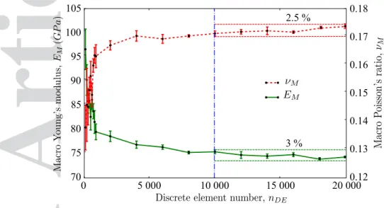
These parameters must be determined by calibration procedure using discrete domains prepared in such a way as to satisfy the geometrical conditions dictated by the structural properties of the modeled continuum, as explained above. Furthermore, these domains must be constructed using at least nDE= 10 000 discrete elements. Indeed, Andr´e et al. [7] have demonstrated in their study

that, for a given set of microscopic parameters (˜rµ,Eµ), the resulting macroscopic elastic behavior

(of the modeled domain) depends upon the number of discrete elements up to approximately nDE = 10 000(fig.2). Beyond this value, the macroscopic elastic properties converge towards limit

values (i.e. the macroscopic behavior becomes nearly independent ofnDE). Therefore, to minimize

the influence of nDE on the calibrated values of the microscopic parameters, discrete domains

made up of at leastnDE = 10 000discrete elements must be used in the calibration procedure. To

simplify this procedure, micro-macro relationships relating the microscopic parameters (Eµandr˜µ)

to the macroscopic elastic properties (EM andνM) were determined numerically, using numerical

samples having the following geometrical settings: average coordination number ncoord= 13.2,

volume fractionvf = 0.68, uniform radius distributionχ = 25%and number of discrete elements

nDE = 10 000. These relationships take the following forms:

˜

rµ = f (νM)

Eµ = g (˜rµ) EM

Accepted

Article

wheref andgare polynomials. Unless otherwise specified, the geometrical settings used to obtain the micro-macro relationships will be held to construct all the discrete domains that will be used in the remainder of the present paper. Using these relationships, tableIpresents the calibrated values ofEµandr˜µcorresponding to silica glass.

0 5 000 10 000 15 000 20 000 0.12 0.13 0.14 0.15 0.16 0.17 0.18 70 75 80 85 90 95 100 105 2.5 % 3 %

Figure 2. Evolution of the macroscopic elastic propertiesEMandνMas a function of the number of discrete elements, for given microscopic beam bond parameters (taken from [7]).

Silica glass macroscopic properties EM = 72 GP a νM = 0.17

Beam bonds microscopic properties Eµ= 129 GP a r˜µ= 0.6

Table I. Silica glass mechanical properties and the associated calibrated microscopic parameters

Using the microscopic parameters of tableI, it is now possible to model the macroscopic elastic behavior of silica glass. The next section deals with the development of an accurate model to describe the densification behavior of this material which is assumed to occur only under hydrostatic pressure.

3. MODELING OF DENSIFICATION UNDER HYDROSTATIC PRESSURE

As seen in the previous section, the DEM variation used in this work models a continuum by a set of rigid spherical particles linked with cohesive beam bonds which model the mechanical behavior of the studied material. Therefore, the natural way to model permanent deformation with this method is to enrich these bonds to take into account such phenomenon. Almost all the models proposed in the literature to model permanent deformation with DEM are based on this way [31,32, 64]. Although these models were successfully applied to simulate permanent deformation of several materials, they suffer from several difficulties. Indeed, they generally involve a large number of calibration parameters, which makes the calibration procedure very challenging. Furthermore, they can only be applied on materials for which the permanent deformation behavior is relatively simple. To overcome these difficulties, the present section proposes a new approach to model permanent

Accepted

Article

deformation of materials with the discrete element method. More specifically, this approach is developed to model densification of materials, e.g. silica glass, under hydrostatic pressure.

The key idea behind this new approach is that, in the framework of traditional continuum methods, several techniques have already been proposed and successfully applied to model complex mechanical behaviors. Therefore, it would be beneficial to apply these techniques for the discrete element method. However, to achieve this aim, it is necessary to establish relationships between certain microscopic (of discrete elements) and macroscopic (of continua) quantities, allowing for discrete-continuum bridging. Pioneering work in this respect has been done by Born and Huang [11] who have used an elastic energy approach to evaluate the stress in lattices by means of the Cauchy-Born hypothesis for homogeneous deformation. Subsequently, other formulations have been proposed to calculate the stress in molecular dynamics (MD). Chief among them is the virial stress which is a generalization of the virial theorem of Clausius (1870) for gas pressure. This formulation has become very popular and widely used in different discrete methods [28]. Therefore, it is retained in this work to bridge the discrete and continuum mechanics in order to develop the new densification model.

3.1. Virial stress

3.1.1. Formulation As originally established [48], the expression of virial stress includes two parts: the first part depends on the mass and velocity (or, in some versions, velocity fluctuation) of the particles; the second part, which provides a continuum measure of the internal mechanical interactions between particles, depends on the inter-particle forces and the particle positions. Using this expression, the average virial stress over a volumeΩaround a particleiis given by:

¯ Π = 1 Ω(−miu˙ i_{⊗ ˙u}i₊1 2 ∑ j̸=i lij⊗ fij) (8)

wheremi andui˙ are respectively the mass and velocity of the particlei,lij = lj− liis the vector

from particle i to particlej,li is the position vector of particle i,fij is the inter-particle force exerted by particlejon particlei, and⊗denotes the tensor product. Expression (8) has been used to compute the stress in discrete systems. Recently, Zhou [72] has demonstrated that this quantity is not a measure for mechanical forces between material points and cannot be regarded as a measure of a mechanical stress. This author has proposed another formulation to compute the average mechanical stress, including only the second part of (8). In a region of volumeΩaround a particlei, the average stress is given by:

¯ σ = 1 2Ω ∑ i∈Ω ∑ j̸=i lij⊗ fij (9)

This expression (9) was developed for molecular dynamics (MD), where the inter-particle forces are only derived from a pair potentialΦ(lij)and the distance between particleslij_{= l}ij

: fij= ∂Φ(l ij₎ ∂lij lij lij (10)

In this case, the resulting stress tensor would be symmetric. However, this cannot be generalized to all other discrete methods. Several papers studying the symmetry of the equivalent stress tensor

Accepted

Article

(obtained using different techniques) in discrete systems can be found in the literature [2,10,15,30]. Based on these papers, in a general case, the symmetry of such a tensor can only be guaranteed when the inter-particle forcesfij are parallel to the vectors linking the particle centerslij. This is particularly true when the particles are linked by spring bonds. This problem is due to the limitations of the existing techniques used in the framework of discrete systems to assess this tensor, which lack accuracy. Further research effort is needed in this direction to get over these limitations. The DEM variation used in this work, where the inter-particle forces are computed based on the cohesive beam bonds, does not guarantee the symmetry of the obtained tensor, although the non-symmetric effects are generally small. A solution to obtain a quasi-symmetric stress tensor with this approach is to assess this tensor by averaging over a large volume that contains a sufficient number of discrete elements. However, this solution makes the calculation of such a tensor very time-consuming and can strongly affect the robustness of any densification model based on this solution. In the present work, a symmetrized form of (9) is used to compute the average stress in a region Ω around a discrete elementi: ¯ σ = 1 2Ω ∑ i∈Ω ∑ j_̸=i 1 2(l ij_{⊗ f}ij + fij⊗ lij) (11)

This solution, which is used in the literature to quickly assess an equivalent stress tensor in discrete systems [8,32,66], generally provides a fair compromise between accuracy and computation cost. Based (11), a Cauchy-like stress tensor can be approximated in each discrete elementias follows:

σi= 1 2Ωi ni ∑ j=1 1 2 ( lij⊗ fij+ fij⊗ lij) (12)

where ni is the number of the discrete elements connected to particle i and Ωi is an effective

volume associated to this particle. The spherical part of this tensor (Pi

num=

1

3tr(σ

i_{)) will be}

used to develop the densification model. Note that this part and then the densification model that will be developed are not influenced by the symmetrization of the stress tensor. The question that arises here is how to choose the effective volumes of the discrete elements so as to ensure that the numerical pressurePi

num in a discrete elementiis equal to the real pressure in this element. The

next subsection tries to answer this question.

3.1.2. Choice of the effective volume of the discrete elements Since the present work deals with

the modeling of densification under hydrostatic pressure, the choice of the effective volumes to be assigned to the discrete elements will be performed taking into account only the spherical part of the Cauchy-like stress (12). These volumes must be determined in such a way as to ensure equality between the numerical pressure computed using (12) and the true pressure in the discrete elements. Due to lack of theoretical basis, there is no analytical approach allowing for obtaining such volumes in a simple and effective manner. The present subsection proposes to investigate this task numerically. Various proposals of effective volumes will be tested using a spherical specimen of100 mm diameter subjected to hydrostatic pressure. This specimen is discretized using10 000

discrete elements. The same microscopic parameters as those presented in tableIare used to model the elastic behavior of the specimen. To evaluate each proposal of effective volume, the evolution of the numerical pressure in the specimen as a function of the specimen volume change will be plotted and commented. To minimize numerical fluctuations, average pressure computed using all

Accepted

Article

the specimen discrete elements (or in some cases using the boundary discrete elements to study the boundary effects) will be used instead of individual discrete element pressures. In the following, the average pressure obtained using all the specimen discrete elements will be referred to as “specimen numerical pressure” and that obtained using only the boundary discrete elements will be referred to as “boundary numerical pressure”.

First, the volume occupied by each discrete element i, which is constant, is chosen to be the effective volume of this elementΩs

i (fig.4): Ωs_i = 4

3π r

3

i (13)

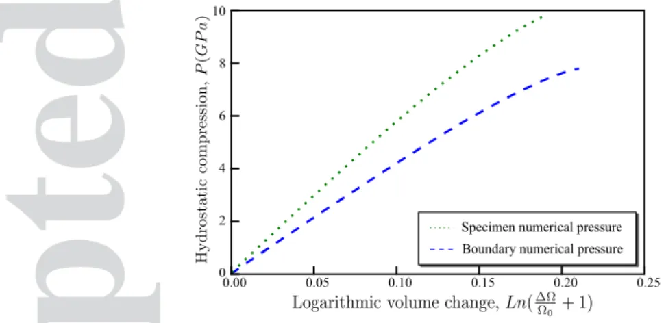
where ri is the radius of the discrete element i. Using (13), figure 3 presents the evolution of

the specimen numerical pressure with the specimen volume change. To investigate the boundary effects, the evolution of the boundary numerical pressure with the specimen volume change is also presented in this figure. Using constant effective volumes, nonlinear dependence between the numerical pressures and the specimen volume change is obtained, which makes no mechanical sense. Furthermore, there is a relatively large difference between the numerical pressure calculated using all the discrete elements and that calculated using only the boundary discrete elements.

0.00 0.05 0.10 0.15 0.20 0.25 0 2 4 6 8 10

Specimen numerical pressure Boundary numerical pressure

Figure 3. Evolution of the specimen numerical pressure and the boundary numerical pressure with the specimen volume change for constant effective volumes

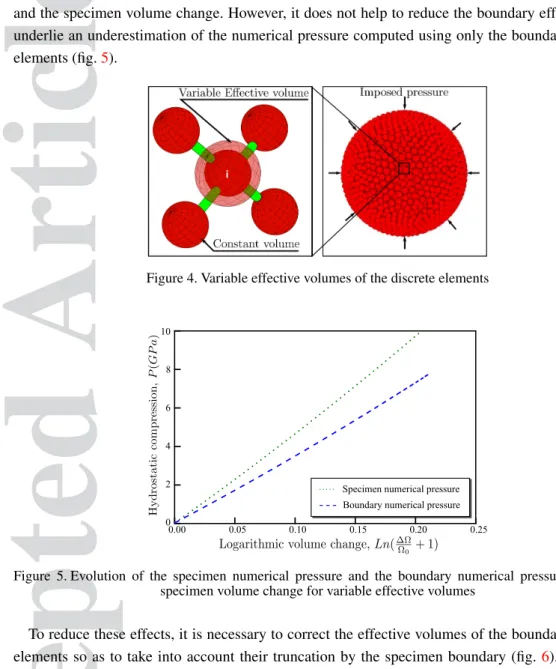
To overcome the problem of nonlinearity, it is necessary to take into account the variation of the effective volumes of the discrete elements with pressure. To this end, the effective volume of each discrete element iis chosen to be the volume of a sphere having as radius (rv

i) half the average

length of the cohesive beam bonds connected to this element (fig.4):

Ωvi = 4 3π (r v i) 3 with riv= 1 ni ni ∑ j=1 lij 2 (14)

whereniis the number of the beams connected to the discrete elementiandlij is the length of the

beam linking discrete elementsiandj. Since the beam lengths vary with the applied pressure, the effective volumes will vary accordingly. Using (14), figure 5shows the evolution of the specimen and the boundary numerical pressures with the specimen volume change. The use of variable effective volumes corrects the problem of nonlinear dependence between the numerical pressure

Accepted

Article

and the specimen volume change. However, it does not help to reduce the boundary effects which underlie an underestimation of the numerical pressure computed using only the boundary discrete elements (fig.5).

Figure 4. Variable effective volumes of the discrete elements

0.00 0.05 0.10 0.15 0.20 0.25 0 2 4 6 8 10

Specimen numerical pressure Boundary numerical pressure

Figure 5. Evolution of the specimen numerical pressure and the boundary numerical pressure with the specimen volume change for variable effective volumes

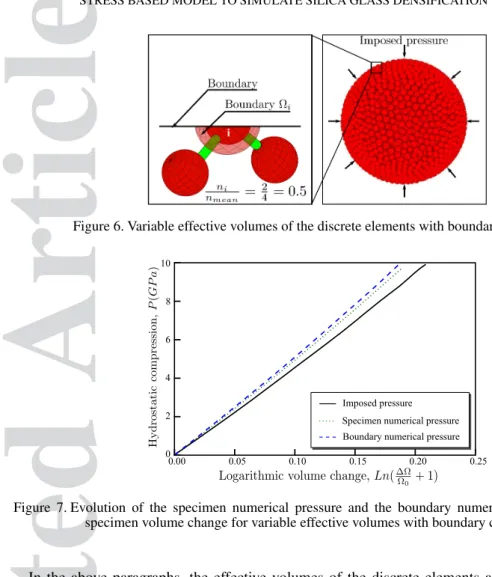
To reduce these effects, it is necessary to correct the effective volumes of the boundary discrete elements so as to take into account their truncation by the specimen boundary (fig. 6). However, this issue is not straightforward. Indeed, it requires prior knowledge of the precise positioning of these elements with respect to the boundary which is generally difficult to draw. To alleviate this problem, the effective volume of each discrete elementi(14) is multiplied by a boundary correction parametercb

i defined as the ratio between the number of the cohesive beams bonds connected to

this element (ni) and the average number of the cohesive beam bonds connected to internal discrete

elements (nmean):

Ωb_i = cb_i× Ωv_i with cb_i = ni

nmean

(15) Figure6illustrates schematically the influence of this parameter. It should be noted that, for internal discrete elements, cb

i is close to1 (cbi ≈ 1). Applying (15), the difference between the numerical

pressure obtained using all the discrete elements and the numerical pressure obtained using only the boundary discrete elements is considerably reduced (fig.7). An error of less than3%is noted between these pressures. This error could be acceptable, especially a few number of discrete elements (only those belonging to the boundary) are affected by it.

Accepted

Article

Figure 6. Variable effective volumes of the discrete elements with boundary correction

0.00 0.05 0.10 0.15 0.20 0.25 0 2 4 6 8 10

Specimen numerical pressure Boundary numerical pressure Imposed pressure

Figure 7. Evolution of the specimen numerical pressure and the boundary numerical pressure with the specimen volume change for variable effective volumes with boundary correction

In the above paragraphs, the effective volumes of the discrete elements are corrected so as to alleviate numerical difficulties related to the boundary effects and the nonlinear pressure dependence of the volume change. The question that arises here is whether the numerical pressure obtained using these corrections would accurately represent the real pressure. To answer this question, the specimen numerical pressure computed using (15) is compared with the hydrostatic pressure imposed on the specimen (fig. 7). An error of approximately 9% is found between the pressures. Since the densification model that will be proposed in the following is based on the pressures in discrete elements, this error must be reduced to ensure a correct functioning of this model. A potential source of such error could be the definition of the effective volumes which should again be corrected to take into account shape irregularity. A final correction is then made to the definition of the effective volumes by multiplying their expressions (15) by a parametercwhich is the same for all the discrete elements:

Ωci = c× Ωbi (16)

The parameter chas to be determined by calibration and can be interpreted as a shape correction parameter that takes into account the shape irregularity of the effective volumes. It is the only one calibration parameter, very easy to calibrate, of the densification model that will be developed in the following. To obtain this parameter, it is sufficient to simulate the response of an elastic numerical sample subjected to hydrostatic pressure, while usingc = 1. The right value ofcis simply the ratio

Accepted

Article

of the specimen numerical pressure to the imposed pressure. The right value ofccorresponding to silica glass can be determined using figure7:c = 1.09. Figure8compares the specimen numerical pressure obtained using this value with the imposed pressure. These pressures are in very close agreement, which proves the validity of the calibrated value of the shape correction parameterc.

0.00 0.05 0.10 0.15 0.20 0.25 0 2 4 6 8 10

Specimen numerical pressure Boundary numerical pressure Imposed pressure

Figure 8. Comparison between the specimen numerical pressure and the hydrostatic pressure imposed on this specimen after shape correction of the effective volumes (c = 1.09)

One major issue generally encountered in discrete methods is that the calibration parameters can depend upon the number of the discrete elements (nDE) used to discretize the numerical sample.

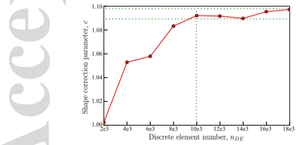
The influence of this number on the calibration of the shape correction parametercmust then be studied. To this end, the same numerical test of spherical specimen under hydrostatic pressure is used with differentnDE(from2 000to18 000). Figure9presents the associated calibration results.

Beyond nDE = 10 000, the calibrated value of c becomes very weakly affected by the discrete

element number. This result is in accordance with the results of Andr´e et al. [7] who have shown that beyondnDE= 10 000the microscopic elastic parameters determined by calibration become

nearly independent ofnDE.

2e3 4e3 6e3 8e3 10e3 12e3

1.00 1.02 1.04 1.06 1.08 1.10

14e3 16e3 18e3

Figure 9. Variation of the shape correction parametercwith the number of the discrete elements used to discretize the numerical sample

In summary, the effective volume that must be assigned to each discrete element i to ensure the equivalence between the numerical pressure and the real pressure in this element is defined as .

Accepted

Article

wherecis a calibration parameter,niis the number of the cohesive beams bonds connected element

i,nmeanis the average number of the cohesive beam bonds connected to internal discrete elements,

andlij _{is the length of the cohesive beam bond linking elementsiandj. Using this definition, it}

would be possible to approximate the pressure in the discrete elements. This opens the floodgates to a new way to model densification with the discrete element method as will be seen in the following subsection.

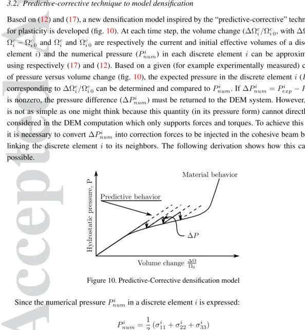
3.2. Predictive-corrective technique to model densification

Based on (12) and (17), a new densification model inspired by the “predictive-corrective” technique for plasticity is developed (fig.10). At each time step, the volume change (∆Ωc_i/Ωc_{i 0}, with∆Ωc_i = Ωc

i − Ωci 0 andΩci and Ωci 0 are respectively the current and initial effective volumes of a discrete

element i) and the numerical pressure (Pi

num) in each discrete element i can be approximated

using respectively (17) and (12). Based on a given (for example experimentally measured) curve of pressure versus volume change (fig.10), the expected pressure in the discrete elementi(Pi

exp)

corresponding to∆Ωc_i/Ωc_{i 0}can be determined and compared toP_numi . If∆P_numi = P_expi − P_numi

is nonzero, the pressure difference (∆Pi

num) must be returned to the DEM system. However, this

is not as simple as one might think because this quantity (in its pressure form) cannot directly be considered in the DEM computation which only supports forces and torques. To achieve this aim, it is necessary to convert∆Pi

numinto correction forces to be injected in the cohesive beam bonds

linking the discrete element i to its neighbors. The following derivation shows how this can be possible.

Figure 10. Predictive-Corrective densification model

Since the numerical pressurePi

numin a discrete elementiis expressed:

P_numi = 1 3(σ i 11+ σ i 22+ σ i 33)

whereσi _{is the stress tensor computed in the discrete elementi,∆P}i

numcan also be expressed as

follows: ∆P_numi = 1 3(∆σ i 11+ ∆σ i 22+ ∆σ i 33) (18)

Accepted

Article

To avoid numerical problems, each∆σi

kk(k∈ [1, 2, 3]) must satisfy: ∆σ_kki ∆Pi num = σ i kk Pi num (19)

Using (19), the correction part of each diagonal term of the stress tensor can be determined. In a similar way,∆σi

kkcan be expressed as:

∆σi_kk=

ni

∑

j=1

∆σ_kkij (20)

whereniis the number of discrete elements connected toiandσkkij is the contribution of the cohesive

beam bond connecting the discrete elementito the discrete elementj in the computation ofσi

kk.

Each∆σij_kkmust also satisfy:

∆σij_kk ∆σi kk =σ ij kk σi kk (21)

Knowing (21), it is possible to determine∆fij that must be introduced in the cohesive beam bond between the discrete elementsiandj:

∆f_kij= 2 Ω c i∆σ ij kk lij_k k∈ [1, 2, 3] (22)

lijis the oriented length of the beam linking the particlesiandjandΩc

i is effective volume of the

discrete elementi(17). Keeping in mind equations (19) and (21), equation (22) can be simplified as follows: ∆fij =∆P i num Pi num fij (23)

The last expression translates ∆Pnumi into correction forces supported by the discrete system

and makes it possible to correct the current mechanical state of the considered discrete element. This is the last step of the “predictive-corrective” densification model proposed in this work. This model presents a great flexibility to reproduce very complex densification behaviors with only one calibration parameter. The next section attempts to apply this model to simulate the densification behavior of silica glass under hydrostatic pressure.

4. APPLICATION: HYDROSTATIC COMPRESSION OF SILICA GLASS

As mentioned in the introduction, silica glass can densify under high hydrostatic pressures. Based on references [36,38,59], the densification behavior of this material takes place between approximately8 GP aand20 GP a, at which the permanent volume change can reach17.4 %. Figure

11 shows the silica glass mechanical behavior under hydrostatic pressure, which is inferred from ex-situ experimental results collected in reference [40]. During this process, the Young’s modulus and the Poisson’s ratio increase with the applied hydrostatic pressure (fig. 12). At the end of densification, these properties show an augmentation of respectively46 %and56 %.

Accepted

Article

Figure 11. Silica glass behavior under hydrostatic pressure (inferred from the experimental results collected in reference [40]) Young's modulus, Poisson's ratio, Y oung's modulus, Poisson's ratio, Hydrostatic compression, 00 05 10 15 20 25 300.0 0.1 0.2 0.3 0.4 0.5 110 100 90 80 70

Figure 12. Variation of the silica glass mechanical properties with pressure (taken from [36])

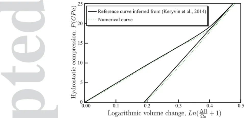
The present section aims to simulate the silica glass densification behavior as well as the associated mechanisms, using the proposed predictive-corrective model. A silica glass sphere of

100 mmdiameter is used in this simulation. This sphere is constructed using the same geometrical settings as presented in section2and discretized using20 000discrete elements. The microscopic elastic parameters of the cohesive beam bonds corresponding to silica glass are given in table I. The shape correction parameter that corresponds to silica glass isc = 1.09. The densification curve presented in figure11 is used as reference curve on which the mechanical state of each discrete element is projected at every time step. Concerning the variation of the silica glass mechanical properties during densification, it is assumed for simplicity in this work that these properties evolve linearly with the applied pressure in the region of densification and remain constant everywhere else (fig.12). Using this assumption, it is very easy to take into account such variation with the proposed predictive-corrective model. For each time step, the hydrostatic pressure in each discrete elementi(Pi

num) is assessed using (12). If8 GP a≤ Pnumi ≤ 20 GP a, this pressure is first corrected

to become equal to the expected pressure in this element (Pi

num= Pexpi ). Then, the macroscopic

mechanical properties associated toPi

expare determined using figure12. Finally, the corresponding

microscopic properties (Ei

Accepted

Article

a cohesive beam bond linking elementsiandjcan be determined and updated as follows:

E_µij = E i µ+ E j µ 2 and r˜ ij µ = ˜ r_µi + ˜r_µj 2 (24)

Taking into account the variation of the mechanical properties with densification, figure 13

presents the response of the silica glass sphere subjected to high hydrostatic compression. The numerical response compares very favorably with the reference one, which means that the developed predictive-corrective model faithfully reproduces the silica glass mechanical behavior. To analyze the evolution of the densification level with the applied pressure, the silica glass sphere is subjected to different hydrostatic pressures. The associated permanent volume changes measured after relaxation are presented in figure14. The numerical results are in very close agreement with the experimental ones obtained by Rouxel et al. [59] and Deschamps et al. [22]. These results are much better than other numerical results obtained in a previous paper [32] using a beam-based densification model. The numerical results obtained in this section shows the great ability of the developed predictive-corrective densification model to simulate the nonlinear mechanical behavior of silica glass, with only one calibration parameter. This model will be used in a future work to study the behavior of silica glass in highly dynamics.

0.00 0.1 0.2 0.3 0.4 0.5 0 5 10 15 20 25

Reference curve inferred from (Keryvin et al., 2014) Numerical curve

Figure 13. Response of the silica glass sphere subjected to hydrostatic compression; comparison between numerical result obtained using the present model and experimental result inferred from ex-situ experimental

data collected in reference [40])

5. CONCLUSION

The present paper dealt with the development of a densification model adapted for DEM to simulate the nonlinear mechanical behavior of silica glass under hydrostatic pressure. This model is based on the computation of a Cauchy-like stress in the discrete elements using a modified expression of the virial stress which is widely used in the literature to assess the stress in discrete systems. One major difficulty in application of this expression to compute the stress in the discrete elements is related to the choice of the effective volumes of these elements. To get over this difficulty, various

Accepted

Article

Exp (Rouxel et al., 2010)

Beam model (Jebahi et al., 2013) Present model

Fitting function

Exp (Deschamps et al., 2013)

Figure 14. Evolution of permanent density change with pressure: comparison between experimental results [22,59], numerical results obtained using the present densification model and numerical results obtained

using a beam-based densification model [32]

proposals of effective volumes were numerically studied. Based on this study, variable effective volumes were retained to ensure linear dependence between the pressure and the volume change in the region of elasticity. The effective volume of each discrete element is chosen to be a sphere having as radius half the average length of the cohesive beam bonds connected to this element. This volume is multiplied by two correction parameters: boundary correction parameter and shape correction parameter. The first parameter is calculated by dividing the number of the cohesive beam bonds connected the considered discrete element by the average number of the cohesive beam bonds connected to internal discrete elements. The second parameter is determined by calibration. After determining this parameter, it is possible to assess the Cauchy-like stress, and then the hydrostatic pressure, in a given discrete element. Using the hydrostatic pressures in the discrete elements, a new densification model inspired by the predictive-corrective technique for plasticity is developed. The mechanical state in each discrete element, given in terms of volume change versus hydrostatic pressure, is determined and corrected with respect to a reference state. To validate this model, it was applied to simulate the silica glass densification behavior which is assumed to occur only under hydrostatic pressure. The associated numerical results are in very close agreement with the experimental results, which proves the effectiveness of the proposed model. Since only one calibration parameter is involved in this model, it is very easy to apply. This new model represents a major step towards accurate modeling of materials permanent deformation with the discrete element method. In a future work, it will be extended to model plasticity of crystalline solids.

ACKNOWLEDGEMENT

This work benefited from the support of the project GLASS ANR-14-CE07-0020 of the French National Research Agency (ANR).

Accepted

Article

1. F. F. Abraham, R. Walkup, H. Gao, M. Duchaineau, T. Diaz De La Rubia, and M. Seager. Simulating materials failure by using up to one billion atoms and the world’s fastest computer: Brittle fracture. Proceedings of the

National Academy of Sciences of the United States of America, 99(9):5777–5782, 2002.

2. N. C. Admal and E. B. Tadmor. A Unified Interpretation of Stress in Molecular Systems. Journal of Elasticity, 100(1):63–143, 2010.

3. B. J. Alder and T. E. Wainwright. Phase Transition for a Hard Sphere System. Journal of Chemical Physics, 27:1208–1209, 1957.

4. B. J. Alder and T. E. Wainwright. Studies in Molecular Dynamics. I. General Method. Journal of Chemical

Physics, 31:459–466, 1959.

5. D. Andr´e. Mod´elisation par ´el´ements discrets des phases d’´ebauchage et de doucissage de la silice. PhD thesis, Universit´e Bordeaux 1, 2012.

6. D. Andr´e, J. L. Charles, and I. Iordanoff. 3D Discrete Element Workbench for Highly Dynamic Thermo-mechanical

Analysis: Gran00. ISTE, London and John Wiley & Sons, 2015.

7. D. Andr´e, I. Iordanoff, J. L. Charles, and J. N´eauport. Discrete element method to simulate continuous material by using the cohesive beam model. Computer Methods in Applied Mechanics and Engineering, 213-216:113–125, 2012.

8. D. Andr´e, M. Jebahi, I. Iordanoff, J. L. Charles, and J. N´eauport. Using the discrete element method to simulate brittle fracture in the indentation of a silica glass with a blunt indenter. Computer Methods in Applied Mechanics

and Engineering, 265:136–147, 2013.

9. A. Arora, D.B. Marshall, B. R. Lawn, and M. V. Swain. Indentation deformation/fracture of normal and anomalous glasses. Journal of Non-Crystalline Solids, 31:415–428, 1979.

10. J. P. Bardet and I. Vardoulakis. The asymmetry of stress in granular media. International Journal of Solids and

Structures, 38:353–367, 2001.

11. M. Born and K. Huang. Dynamical Theory of Crystal Lattices. Oxford, Clarendon, 1954.

12. P. W. Bridgman and I. ˇSimon. Effects of Very High Pressures on Glass. Journal of applied physics, 24(405), 1953. 13. R. Br¨uckner. Properties and structure of vitreous silica. I. Journal of Non-Crystalline Solids, 5(2):123–175, 1970. 14. R. Br¨uckner. Properties and structure of vitreous silica. II. Journal of Non-Crystalline Solids, 5(3):177–216, 1971. 15. B. Cambou, M. Jean, and F. Radja. Micromechanics of Granular Materials. Wiley, 2001.

16. E. B. Christiansen, S. S. Kistler, and W. B. Gogarty. Irreversible Compressibility of Silica Glass as a Means of Determining the Distribution of Force in High-pressure Cells. Journal of the American Ceramic Society, 45(4):172– 177, 1962.

17. H. M. Cohen and R. Roy. Effects of Ultra high Pressures on Glass. Journal of the American Ceramic Society, 44(10):523–524, 1961.

18. H. M. Cohen and R. Roy. Reply to “Comments on‘Effects of Ultrahigh Pressures on Glass’”. Journal of the

American Ceramic Society, 45(8):398–399, 1962.

19. P. A. Cundall. Computer Model for Simulating Progressive Large Scale Movements in Blocky Rock Systems. In

Proceedings of the Sym posium of the International Society of Rock Mechanics , Nancy, France, 1971.

20. P. A. Cundall and O. D. L. Strack. A discrete numerical model for granular assemblies. G´eotechnique, 29(1):47– 65, 1979.

21. F. Dachille and R. Roy. High Pressure Studies of the Silica Isotypes. Zeitschrift Kristallographie, 111:451–461, 1959.

22. T. Deschamps, A. Kassir-Bodon, C. Sonneville, J. Margueritat, C. Martinet, D. de Ligny, A. Mermet, and B. Champagnon. Permanent densification of compressed silica glass: a raman- density calibration curve. Journal

of Physics: Condensed Matter, 25:25402–25405, 2013.

23. J. L. Finney. Random packings and the structure of simple liquids. i. the geometry of randomclose packing.

Proceedings of the Royal Society of London. Series A, Mathematical and Physical Sciences, 319(1539):479–493,

1970.

24. W. M. C. Foulkes, L. Mitas, R. J. Needs, and G. Rajagopal. Quantum Monte Carlo simulations of solids. Reviews

of Modern Physics, 73(1), 2001.

25. K. Gotoh and J. L. Finney. Statistical geometrical approach to random packing density of equal spheres. Nature, 252:202–205, 1974.

26. S. Grimme. Accurate description of van der Waals complexes by density functional theory including empirical corrections. Journal of Computational Chemistry, 25(12):1463–1473, 2004.

27. T. M. Gross. Deformation and cracking behavior of glasses indented with diamond tips of various sharpness .

Journal of Non-Crystalline Solids, 358(24):3445–3452, 2012.

28. H. Haddad, W. Leclerc, M. Guessasma, C. P´elegris, N. Ferguen, and E. Bellenger. Application of DEM to predict the elastic behavior of particulate composite materials . Granular Matter, 17:459–473, 2015.

Accepted

Article

29. W. J. Hehre. A Guide to Molecular Mechanics and Quantum Chemical Calculations. Wavefunction Press, Irvine, CA, 2003.

30. A. Ian Murdoch. A Critique of Atomistic Definitions of the Stress Tensor. Journal of Elasticity, 88:113–140, 2007. 31. M. Jebahi. Discrete-continuum coupling method for simulation of laser-inducced damage in silica glass. PhD

thesis, Bordeaux 1 University, 2013.

32. M. Jebahi, D. Andr´e, F. Dau, J. L. Charles, and I. Iordanoff. Simulation of Vickers indentation of silica glass.

Journal of Non-Crystalline Solids, 378:15–24, 2013.

33. M. Jebahi, D. Andr´e, I. Terreros, and I. Iordanoff. Discrete Element Method to Model 3D Continuous Materials. ISTE, London and John Wiley & Sons, 2015.

34. M. Jebahi, F. Dau, J. L. Charles, and I. Iordanoff. Discrete-continuum Coupling Method to Simulate Highly

Dynamic Multi-scale Problems: Simulation of Laser-induced Damage in Silica Glass. ISTE, London and John

Wiley & Sons, 2015.

35. M. Jebahi, A. Gakwaya, J. L´evesque, O. Mechri, and K. Ba. Robust methodology to simulate real shot peening process using discrete-continuum coupling method. International Journal of Mechanical Sciences, 107:21–33, 2016.

36. H. Ji. M´ecanique et physique de l’indentation du verre . PhD thesis, Universit´e de Rennes 1, 2007.

37. L. Jing and O. Stephansson. Fundamentals o f Discrete Element Methods for Rock Engineering: Theory and

Applications. Elsevier, 2007.

38. V. Keryvin. Contribution `a l’´etude des m´ecanismes de d´eformation et de fissuration des verres, 2008. Habilitation `a diriger des recherches, Universit´e de Rennes 1.

39. V. Keryvin, S. Gicquel, L. Charleux, J. P. Guin, M. Nivard, and J. C. Sangleboeuf. Densification as the only mechanism at stake during indentation of silica glass? Key Engineering Materials, 606:53–60, 2014.

40. V. Keryvin, J. X. Meng, S. Gicquel, J. P. Guin, L. Charleux, J. C. Sangleboeuf, P. Pilvin, T. Rouxel, and G. Le Quilliec. Constitutive modeling of the densification process in silica glass under hydrostatic compression. Acta

Materialia, 62:250–257, 2014.

41. A. Lisjak and G. Grasselli. A review of discrete modeling techniques for fracturing processes in discontinuous rock masses. Journal of Rock Mechanics and Geotechnical Engineering, 6:301–314, 2014.

42. G. R. Liu and M. B. Liu. Smoothed particle hydrodynamics : a meshfree particle method. World Scientific Publishing Co. Pte. Ltd, 2003.

43. M. B. Liu and G.R. Liu. Smoothed Particle Hydrodynamics (SPH): an Overview and Recent Developments.

Archives of computational methods in engineering, 17:25–76, 2010.

44. G. Lu and E. Kaxiras. Handbook of Theoretical and Computational Nanotechnology, chapter Overview of

Multiscale Simulations of Materials. American Scientific Publishers, rieth, m. and schommers, w. edition, 2005. 45. J. D. Mackenzie. High-Pressure Effects on Oxide Glasses: I, Densification in Rigid State. Journal of the American

Ceramic Society, 46(10):461–470, 1963.

46. O. K. Mahabadi, A. Lisjak, A. Munjiza, and G. Grasselli. Y-Geo: new combined finite-discrete element numerical code for geomechanical applications. International Journal of Geomechanics, 12:676–688, 2012.

47. C. L. Martin, D. Bouvard, and S. Shima. Study of particle rearrangement during powder compaction by the discrete element method. Journal of the Mechanics and Physics of Solids, 51(4):667–693, 2003.

48. A. G. McLellan. Virial theorem generalized. American journal of physics, 42(239), 1974.

49. T.A. Michalske and S.W. Freiman. A molecular mechanism for stress corrosion in vitreous silica. Journal of the

American Ceramic Society, 66(4):284–288, 1983.

50. A. Munjiza. The combined Finite-Discrete Element Methode. John Wiley & Sons, 2004.

51. K. Muralidharan, J. H. Simmons, P. A. Deymier, and K. Runge. Molecular dynamics studies of brittle fracture in vitreous silica: Review and recent pregress . Journal of Non-Crystalline Solids, 351:1532–1542, 2005.

52. T. P¨oschel and T. Schwager. Computational Granular Dynamics: Models and Algorithms. Springer, 2005. 53. D. O. Potyondy. Bonded-particle modeling of fracture and flow. In Frontiers in Particle Science and Technology:

Mitigation and Application of Particle Attrition, pages 65–120, 2016.

54. D. O. Potyondy and P. A. Cundall. Abonded-particle model for rock. International Journal of Rock Mechanics &

Mining Sciences, 41:1329–1364, 2004.

55. D.O. Potyondy. The bonded-particle model as a tool for rock mechanics research and application: current trends and future directions. Geosystem Engineering, 18(1):1–28, 2015.

56. P. W. Randles and L. D. Libersky. Smoothed particle hydrodynamics: Some recent improvements and applications.

Computer Methods in Applied Mechanics and Engineering, 139:375–408, 1996.

57. E. Rougier, E. E. Knight, A. J. Sussman, R. P. Swift, and C. R. Bradley. The combined finite-discrete element method applied to the study of rock fracturing behaviour in 3D. In Proceedings of the 45th US Rock

Accepted

Article

58. E. Rougier, A. Munjiza, and N. W. M. John. Numerical comparison of some explicit time integration schemes used in DEM, FEM/DEM and molecular dynamics. International journal for numerical methods in engineering, 62:856–879, 2004.

59. T. Rouxel, H. Ji, F. Augereau, and B. Ruffl´e. Indentation deformation mechanism in glass: Densification versus shear flow. Journal of applied physics, 107, 2010.

60. T. Rouxel, H. Ji, T. Hammouda, and A. Mor´eac. Poisson’s Ratio and the Densification of Glass under High Pressure.

Physical Review letters, 2008.

61. E. Schlangen and J. G. M. van Mier. Experimental and numerical analysis of micromechanisms of fracture of cement-based composites. Cement and Concrete Composites, 14(2):105–118, 1992.

62. E. Schlangen and J. G. M. van Mier. Simple lattice model for numerical simulation of fracture of concrete materials and structures. Materials and Structures, 25(9):534–542, 1992.

63. C. Sonneville, T. Deschamps, C. Martinet, D. de Ligny, A. Mermet, and B. Champagnon. Polyamorphic transitions in silica glass. Journal of Non-Crystalline Solids, 382:133–136, 2013.

64. I. Terreros. Mod´elisation DEM thermo-m´ecanique d’un milieu continu. Vers la simulation du proc´ed´e FSW. PhD thesis, ´Ecole Nationale Sup´erieure d’Arts et M´etiers, 2013.

65. S. P. Timoshenko. History of Strength of Materials: With a Brief Account of the History of Theory of Elasticity and

Theory of Structure. Dover, New York, NY, 1983.

66. P. Viot, I. Iordanoff, and D. Bernard. Multiscale description of polymeric foam behavior: A new approach based on discrete element modeling. Polymer Science Series A, 50(6):679–689, 2008.

67. C. E. Weir and S. Spinner. Comments on “Effects of Ultrahigh Pressures on Glass”. Journal of the American

Ceramic Society, 45(4):196, 1962.

68. S. M. Wiederhorn. Influence of Water Vapor on Crack Propagation in Soda-Lime Glass. Journal of the American

Ceramic Society, 50(8):407–414, 1967.

69. S. M. Wiederhorn and J. P. Guin. Fracture of silicate glasses: ductile or brittle? Physical Review letters,

92(21):215502, 2004.

70. C. Yan, H. Zheng, G. Sun, and X. Ge. Combined Finite-Discrete Element Method for Simulation of Hydraulic Fracturing. Rock Mechanics and Rock Engineering, 49(4):1389–1410, 2016.

71. S. Yoshida, J. C. Sangleboeuf, and T. Rouxel. Quantitative evaluation of indentation-induced densification in glass.

Journal of Materials Research, 20(12), 2005.

72. M. Zhou. A new look at the atomic level virial stress: on continuum-molecular system equivalence. Proceedings

of the Royal Society A, 459:2347–2392, 2003.

73. O. C. Zienkiewicz and R. L. Taylor. The Finite Element Method for Solid and Structural Mechanics. Elsevier, 2005.