HAL Id: halshs-03123659
https://halshs.archives-ouvertes.fr/halshs-03123659
Preprint submitted on 4 Feb 2021
HAL is a multi-disciplinary open access
archive for the deposit and dissemination of sci-entific research documents, whether they are pub-lished or not. The documents may come from teaching and research institutions in France or abroad, or from public or private research centers.
L’archive ouverte pluridisciplinaire HAL, est destinée au dépôt et à la diffusion de documents scientifiques de niveau recherche, publiés ou non, émanant des établissements d’enseignement et de recherche français ou étrangers, des laboratoires publics ou privés.
Urbanisation and the onset of modern economic growth
Liam Brunt, Cecilia García-Peñalosa
To cite this version:
Liam Brunt, Cecilia García-Peñalosa. Urbanisation and the onset of modern economic growth. 2021. �halshs-03123659�
Working Papers / Documents de travail
WP 2021 - Nr 01
Urbanisation and the onset of modern economic growth
Liam Brunt Cecilia García-Peñalosa
0
Urbanisation and the onset of modern economic growth
*Liam Brunt a
Norwegian School of Economics and CEPR and
Cecilia García-Peñalosa b
Aix-Marseille University, CNRS, EHESS, AMSE, and CEPR
January 2021
Abstract: A large literature characterizes urbanisation as the result of productivity growth attracting rural workers to cities. We incorporate economic geography elements into a growth model and suggest that causation runs the other way: when rural workers move to cities, the resulting urbanisation produces technological change and productivity growth. Urban density leads to knowledge exchange and innovation, thus creating a positive feedback loop between city size and productivity that sets off sustained economic growth. The model is consistent with the fact that urbanisation rates in Western Europe, and notably in England, reached unprecedented levels by the mid-18th century, the eve of the Industrial Revolution.
Key words: Industrialization, urbanisation, innovation, long-run growth. JEL codes: N13, O14, O41.
* This paper has benefited from comments at seminars and workshops at AMSE, the University of Alicante, Bocconi University, Brown University, the Institute of Economic Analysis (Barcelona), the Paris School of Economics, the University of Zurich, the CEPR conference “Accounting for the Wealth of Nations” in Odense and the Workshop in Honor of Steve Turnovsky in Vienna, as well as from discussions with Sacha Becker, Raouf Boucekkine, David de la Croix, Jakob Madsen, Omer Moav, Fidel Pérez Sebastián, Romain Rancier, Eric Roca Fernández, Tanguy van Ypersele, and Lucy White. We are particularly grateful to the editor and reviewers of this Journal and to Greg Spanos for his assistance. This work was partly supported by French National Research Agency Grant ANR-17-EURE-0020.
a Email: liam.brunt@nhh.no
1 1. Introduction
Urbanisation and technological progress are closely linked. Economic historians and development economists have widely documented how workers are drawn to cities from the traditional sector in order to profit from the modern technologies that are created and adopted there.1 Models of long-run growth thus tend to see urbanisation as a consequence of economic growth. At the same time, a vast literature on economic geography maintains that urbanisation itself generates productivity gains: going back to Marshall, economists have explored the idea that high density in cities results in learning – and thus in both skill upgrading and in innovation.2 This suggests that agglomeration can cause economic growth through its impact on technological change. The aim of this paper is to model the two-way relationship between urbanisation and innovation in order to understand how they interacted at the onset of modern economic growth.
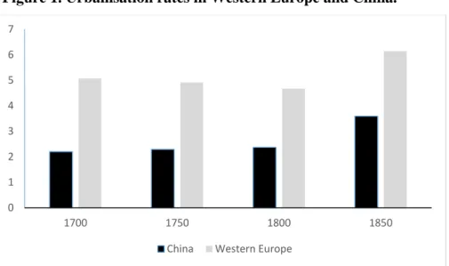
Our analysis is motivated by the observation that Europe was unusually urbanised before the Industrial Revolution. China is regarded by many historians as the most technologically advanced country in the Middle Ages.3 However, despite an early upsurge in the share of population living in cities, urbanisation rates remained low throughout the modern period, as argued by Maddison (2007) and Voigtländer and Voth (2013b). By contrast, Western Europe experienced a marked increase in the share of population living in cities during the early modern period, already exhibiting an urbanisation rate of 5% by 1700, more than twice that prevailing in China, as shown in figure 1.
Figure 1. Urbanisation rates in Western Europe and China.
Source: Authors calculations, see below.
1 See, for example, Harris and Todaro (1970), Rosenberg and Trajtenberg (2004) for an analysis of the effect of technological adoption on urbanisation in the 19th century, and Temple (2005) for a review.
2 See Marshall (1890) as well as Glaeser (1999) and Combes, Mayer and Thisse (2008). 3 Needham (1954) and his colleagues offered the seminal contribution here.
0 1 2 3 4 5 6 7 1700 1750 1800 1850 China Western Europe
2
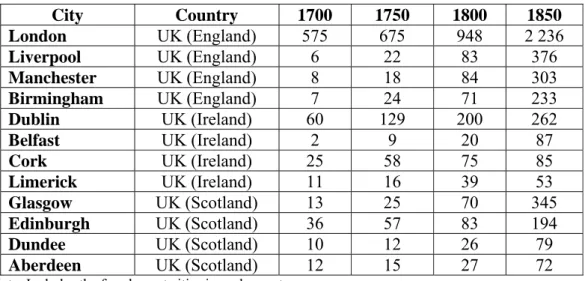
Interestingly, England was a significant outlier in the European urbanisation experience, with much higher rates than we would expect. Note further that the share of people living in cities had started to expand at a considerable pace well before the First Industrial Revolution. For example, the urbanisation rate had already risen threefold between 1600 and 1750, from 6 to 18% (Wrigley et al., 1997). Table 1 shows the four largest cities in each of England, Scotland and Ireland, all part of the UK at that time. It indicates that the UK experienced an urban growth spurt before 1750, i.e. before the First Industrial Revolution. Whilst the population of London rose by 17%, the population of almost all the other cities reported doubled or tripled in the first half of the 18th century; by contrast, the English population increased by only 14% (Wrigley and Schofield, 1981).4 We present more extensive urbanisation data for England and other countries in the next section. Yet the timing of these increases certainly raises the question of the extent to which urbanisation was a cause – rather than a consequence – of economic growth.
Table 1. Expansion over time of the largest UK cities (population in `000s).
City Country 1700 1750 1800 1850 London UK (England) 575 675 948 2 236 Liverpool UK (England) 6 22 83 376 Manchester UK (England) 8 18 84 303 Birmingham UK (England) 7 24 71 233 Dublin UK (Ireland) 60 129 200 262 Belfast UK (Ireland) 2 9 20 87 Cork UK (Ireland) 25 58 75 85 Limerick UK (Ireland) 11 16 39 53 Glasgow UK (Scotland) 13 25 70 345 Edinburgh UK (Scotland) 36 57 83 194 Dundee UK (Scotland) 10 12 26 79 Aberdeen UK (Scotland) 12 15 27 72
Note: Includes the four largest cities in each country. Source: Bairoch et al. (1988); De Vries (1984).
In this paper, we develop a model of growth consistent with the idea that urbanisation precedes industrialisation. The first element in our setup is a two-sector model where agriculture takes place in rural areas and manufacturing activity in cities. The manufacturing sector is modelled as a traditional artisan activity rather than modern industrial production, without the use of physical capital, and with the productivity of a worker depending only on the number of ideas that he holds. As the average number of ideas available grows, manufacturing productivity increases, and the incentives to leave the
3
countryside rise, leading to higher employment in manufacturing, as, for example, in Hansen and Prescott (2002). Our second element consists in modelling how ideas appear and are transmitted. We model the transmission of ideas between agents through imitation: individuals in cities may acquire an idea by meeting someone who already possess it. We also suppose that an individual can create a
novel idea by observing the ideas or experience of others, thus endogenously inventing new ways of
production, in line with Jovanovic and Rob (1989). In either case, acquiring ideas is the result of meetings between individuals. We follow Marshall and the formalization of his approach by Glaeser (1999, 2011) and suppose that the number of meetings is an increasing function of urban density. Higher density implies more meetings and hence more imitation and innovation; in contrast, the low density in rural areas implies that there are no meetings and hence no transmission or creation of ideas. Under these assumptions, the rate of urbanisation becomes the determinant of manufacturing productivity.
Two key results emerge. First, the above two elements together suffice to create a feedback mechanism between city size and technology that generates a novel set of growth dynamics. A shock to urbanisation results in knowledge creation and diffusion, higher manufacturing productivity, and a flow of labour into manufacturing and hence into cities. The resulting higher urban density further increases manufacturing productivity, thus setting off a process of increasing urbanisation and innovation that generates sustained growth. Thus our model makes urbanisation – as opposed to industrialization – the key element in a theory of development. Second, the microfounded process of knowledge generation allows us to dissociate the creation of ideas from their diffusion. Because an idea is invented by an individual, initially only the inventor holds that idea, which will then be transmitted to agents of the next generations through imitation. Those individuals who have not managed to imitate others will not be able to use the most recent technology, implying only a moderate increase in productivity. However, since now the idea is held by more individuals than just the innovator, it can be imitated by a larger number amongst the young of the next generation, further increasing the share of manufacturing workers who can use. As a result an innovation will increase productivity only slowly as imitation by subsequent generations occurs. This generates a model that can simultaneously deliver fast technological change and slow overall productivity growth in manufacturing, in line with existing estimates for the 18th and 19th centuries (see Crafts, 2004).
We calibrate our model to reproduce a number of features of the English economy over three centuries. In doing so, we consider possible reasons why England was highly urbanised. A number of aspects have been discussed in the literature, going from location fundamentals to military conflict
4
and the Black Death.5 While any of the above mechanisms could have been a trigger for the sustained growth model that we develop, our analysis will emphasize the role of agricultural sector triggers, as our setup implies that high urbanisation is associated with high labour productivity in agriculture, a phenomenon that was particularly important in England. As we document below, England was both more urbanised and had higher agricultural labour productivity than other Western European countries; and Western Europe was, on average, more urbanised and had higher agricultural labour productivity than China. Thus, increasing agricultural productivity is a candidate trigger for a growth take off. The period is also characterised by changes in in the share of agricultural output that went to the landlord and the taxman, i.e. in agricultural extractions. The role of agricultural extractions as an additional shock during early modern times has received little attention in the literature, yet it seems to us to have been particularly relevant in the case of England. High extractions from agriculture were the result of two phenomena. On the one hand, the established land property system in Northern Europe implied that a substantial amount of production went to the owner of the land, who was generally not the one who worked it. On the other hand, in 17th and 18th century Europe, tax revenues were rising fast – particularly in England – and the main source of this tax revenue was the agricultural sector.6 Our model will therefore explore shocks to both the knowledge generation process and to the agricultural sector – in the form of higher productivity and higher extractions – and examine their joint implications for urbanisation and growth.
Our paper is related to several strands of literature. First is the recent development in growth theory explaining how the world moved from stagnation to growth, best represented by Unified Growth Theory (UGT); see Galor and Weil (2000) and Galor (2011). UGT is at the core of our understanding of the appearance of modern growth and of the close relationship between population dynamics and economic development. And yet, specific differences in the timing and speed of the transition are still not fully understood. A number of recent papers have focussed on the unique features of Europe, and particularly England, before the Industrial Revolution.7 For example, Desmet and Parente (2012) emphasize the role of market size and argue that markets in England were more integrated – and thus larger – than elsewhere by the early 18th century, and this allowed firms to implement cost-reducing production technologies. Our analysis is closely related to Voigtländer and
5 See section 5 below for further discussion.
6 For evidence on historical fiscal patterns see Karaman and Pamuk (2010), Dincecco (2011) and Voigtläder and Voth (2013b). Karaman and Pamuk (2010), figure 5, show that, across Europe, per capita tax revenues were highest in England and the Dutch Republic in the 18th century, the Netherlands also being a highly urbanised country. For an exhaustive account of the English tax system and its reliance on agricultural sector taxes, see Dowell (1884).
7 The literature by economic historians on the First Industrial Revolution is obviously very extensive; see Mokyr (2008, 2009) for a recent discussion.
5
Voth (2006, 2013a). Both of their models share with ours an approach based on the migration of workers from agriculture into manufacturing. Voigtländer and Voth (2006) identify the importance of demographic patterns in countries like France and England for the prospects of industrialization, while Voigtläder and Voth (2013a) maintain, like we do, that cities played a crucial role in early modern times. In their setup, the Black Death is the exogenous trigger that initially raises wages and results in migration towards cities, with the poor health conditions in cities then increasing average mortality rates and allowing Europe to escape from the Malthusian trap. Our analysis complements theirs by maintaining that the frequent interactions occurring in cities not only resulted in the transmission of viruses but also of ideas. Lastly, Boucekkine, Peeters and de la Croix (2007) also consider the role of population density and argue that it reduced the cost of attending and creating schools, thus increasing educational investments. Their analysis abstracts from technological change, which is the focus of our model.
The determinants of technological change have been extensively examined in the endogenous growth literature, which sees population size, production externalities or intentional R&D as sources of productivity improvement. We depart from these approaches and add to a small literature which, starting with Lucas (2009), considers the role of individually-held knowledge. Lucas maintains that the onset of modern growth is linked to the appearance of a class of individuals that “spend entire careers exchanging ideas, solving work‐related problems, generating new knowledge” (Lucas, 2009, p.1), and develops a growth model in which each individual learns from all others in the same economy. This concept has been applied to different spaces for the transmission of ideas, notably firms, schooling or trade; see Alvarez et al. (2013), Buera and Lucas (2018), Caicedo et al. (2019). For example, international trade is growth-enhancing because it puts domestic producers in contact with more efficient foreign firms. We share with these works an emphasis on the contribution of human interaction to knowledge flows and the role played by random meetings. However, we consider a different source of interactions by focusing on the physical proximity provided by city life, a context that is particularly suitable when thinking about early modern growth.
Our paper is also related to the vast literature on how urban growth relates to aggregate GDP growth. Early development economists saw the shift of resources from an agricultural to an urban, modern sector as the key element in the growth process; see Lewis (1954) and Harris and Todaro (1970). These models assumed an exogenous modern, urban technology and a backward rural one. The presence of some form of friction – such as migration restrictions or wage subsidies – limited the flow of workers into the city, and delivered predictions on how these policies simultaneously affected
6
urbanisation and the level of GDP. In the 1990s, more complex dual economy models enriched the basic framework, but shared with the early work the assumption that ongoing urbanisation results from exogenous forces, notably exogenous technological change favoring the urban sector and falling transportation costs (see, for example, Bencivega and Smith, 1997). As a result, these models are useful for examining the policies that jeopardize urbanisation and output growth, but have the drawback that there are no endogenous agglomeration forces. This question has been addressed by the economic geography literature. One strand of the literature uses core-periphery models to examine how city size is determined by the presence of scale economies in production (see Henderson, 2005, for a review), while an alternative approach has focused on the idea that agglomeration leads to knowledge diffusion and creation (Glaeser, 1999). Yet, the focus in both cases is on the relative size of cities, rather than the rural-urban divide associated with an agricultural/manufacturing dichotomy and its implications for growth. Our model combines these two approaches, endogenizing the rural-urban productivity gap by introducing the elements found in economic geography into a dual economy model.
Following the argument first put forward by Marshall (1890) and the seminal work of Jacobs (1969), numerous authors have modelled how the environment offered by cities improves the prospects for generating and diffusing new ideas. Cities affect the productivity of firms and workers as they generate technology spillovers across firms, and learning and skill-acquisition by workers. Various mechanisms can give rise to innovation and learning in cities; see Duranton and Puga (2004) for a review. One of the most influential arguments has been the idea that proximity to individuals with greater skills or knowledge facilitates the exchange and diffusion of knowledge. In this context, higher urban density results in more frequent encounters and thus leads to greater transmission of skills and ideas between workers. Our paper uses the insights of this vast literature to model the process of imitation and innovation that takes place in cities. In line with empirical findings,8 we assume a process of knowledge creation in which innovation and productivity both increase with urban density, and by introducing these into a fully-fledged growth model we can examine the long-term implications of such learning.
The rest of the paper is organised as follows. The next section provides a more detailed discussion of the historical evidence that supports our arguments. Section 3 presents our two-sector model and examines the determinants of urbanisation. Section 4 considers the mechanism for the creation and transmission of ideas, and incorporates them into our macroeconomic model in order to
7
obtain the joint dynamics of urbanisation and knowledge. In section 5 we discuss our model in the light of existing evidence, while section 6 provides numerical examples and calibrates the model to show that its predictions match the data available for England. We conclude in section 7.
2. The historical context
As we detail in the next section, our model links the observed spatial and temporal variation of three key variables: urbanisation levels, agricultural labour productivity and output growth. In this section we describe the salient features of two of these variables, examining urbanisation and agricultural productivity across Western Europe and China in the 18th and 19th centuries. Since a vast literature has documented the takeoff experienced in England and Europe, we refrain from discussing this aspect here.9 We start by showing that urbanisation rates were higher in Western Europe than in China before the Industrial Revolution; and, within Europe, England was particularly urbanised. Then we will see that high urbanisation rates were accompanied by high agricultural labour productivity. While Europe’s extraordinary urbanisation made it a likely candidate for an early transition to modern growth, we will see that England was unique in both dimensions by 1750, as it experienced high and growing preindustrial urbanisation, accompanied by high agricultural labour productivity.
Patterns of urbanisation
Measuring urbanisation is not straightforward because there is no consensus on what population threshold defines a city. For example, Bairoch et al. (1988) use a cutoff of 5 000 inhabitants, while De Vries (1984) reports data for all European towns and cities larger than 10 000. But most of us would probably think of cities as being larger conurbations than this, even in the Middle Ages. Moreover, Chinese data are available only for larger cities. Hence we use 200 000 inhabitants as the cutoff for the descriptive statistics that we present here, in order to ensure comparability and accuracy across space and over time. Although our model does not guide us to prefer one cutoff over another, we believe that agglomeration externalities exist in cities of less than 200 000 inhabitants and therefore we use the 10 000 threshold whenever possible, such as in our simulations for England below.
9 See, amongst others, Crafts (2004) and Broadberry and O’Rourke (2010). We will return to output dynamics in our calibration exercise.
8
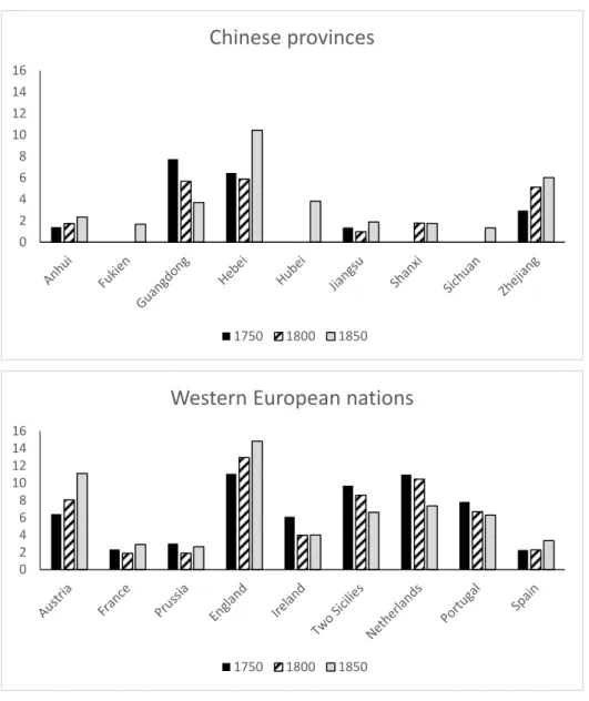
Figure 2. Shares of urban population in Chinese provinces and Western European nations.
Sources: Chandler and Fox (1974), Skinner (1977), and De Vries (1984). See Appendix A for details.
Figure 2 presents the share of population living in cities in China and Western Europe. The sizes of Chinese provinces are roughly comparable to European countries, so the units of analysis are not too disparate. We include all provinces/nations that had at least one city reaching a population of 200 000 at some point during the period of analysis, and we compute urbanisation rates as the sum of all inhabitants in such cities divided by the total population of the province/nation. Appendix A (tables A.1 to A.6) provides further details on the data, as well as the list of cities that we consider. Figure 2 indicates that, on the eve of industrialization, Western Europe had reached considerably higher levels of urbanisation than China. In 1750, the two most urbanised Chinese provinces, Guangdong (home of Canton/Guangzhou) and Hebei (home of Peking/Beijing), had urbanisation rates of 8 and 6% – well
0 2 4 6 8 10 12 14 16
Chinese provinces
1750 1800 1850 0 2 4 6 8 10 12 14 16Western European nations
1750 1800 18509
below the 11% found in England and the Netherlands. Moreover, while only two Chinese provinces had urbanisation rates above 3%, in Europe it was not only England and the Netherlands that had reached at least twice this rate but also Austria, the Kingdom of the Two Sicilies (the largest of the Italian states before unification), Ireland, and Portugal. In 1750, the (population-weighted) average urbanisation rate among the Chinese provinces was 2.29% while that for the European nations was twice as high, at 4.82%. By 1850, China and Western Europe reached 3.59% and 6.26%, respectively (see Appendix A).
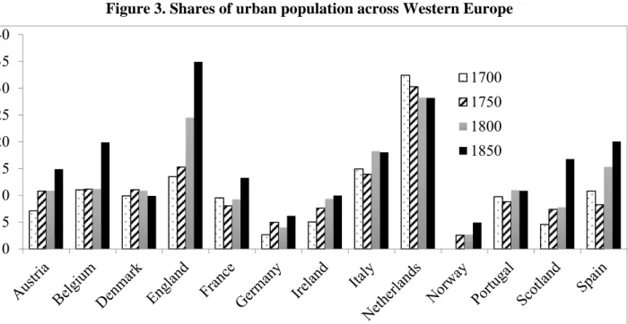
Figure 3. Shares of urban population across Western Europe
Source: Bairoch et al. (1988), De Vries (1984) and Brunt and Fidalgo (2008). See Appendix A for details.
Among the Western European nations, England had the highest urbanisation rate, with 11% of the population living in large (i.e. greater than 200 000) cities, followed closely by the Netherlands and Italy. Figure 3 presents an alternative measure of urbanisation. It uses De Vries’ definition of cities as agglomerations of 10 000 or more inhabitants. Using this cutoff allows us to incorporate a number of other European nations that did not have, at that time, cities above 200 000 inhabitants. Adopting a lower threshold for the definition of a city obviously counts many more people as urbanites, and thus generates urbanisation rates considerably higher than in the previous figure. When considering medium-sized cities, the Netherlands dominates all other countries by a vast margin, with England exhibiting the second highest urbanisation rate in 1750 at 15.3%. This figure is well above that of other large nations, such as France or Spain, where urbanisation was only around 8%. Urbanisation was also
0 5 10 15 20 25 30 35 40 1700 1750 1800 1850
10
high in Italy and Belgium.10 Note that Belgium was the first country in Continental Europe to industrialize, following England quite closely, while the fact that the Netherlands experienced a relatively late industrialization has been seen as a puzzle by historians (Mokyr, 1999).
So far, our discussion has focused on variations in the level of urbanization across space. But we also need to consider the change in urbanization over time. The traditional approach sees urbanisation as the result of productivity growth, which implies that urban growth should have started
after the increased innovation that we see in the Industrial Revolution. In our model, too, higher
innovation will cause urbanization because an increase in either agricultural or manufacturing productivity raises urbanisation. In consequence, an exogenous increase in agricultural or manufacturing TFP (such as Hargreaves’ 1764 invention of the “Spinning Jenny” for producing cotton thread) would have the effect of triggering a flow of labour into the city. Alternatively, shocks that accelerate the diffusion of ideas within cities would, for given knowledge, increase productivity. For example, there might be more encouragement for innovators to meet – as with the foundation of the Royal Society for the Encouragement of Arts, Manufactures and Commerce in London in 1754. Or there might be improved access to technical literature – such as the appearance of Chamber’s
Cyclopaedia: An universal dictionary of arts and sciences (the first modern encyclopaedia, which was
published in London in 1728). Mokyr (2004) offers many other examples of this type of propagation of ‘useful’ knowledge. But these developments occurred too late to explain English urbanisation, which had already tripled between 1600 and 1750 (from 6 to 18% of the population), indicating that something else must have prompted increased urbanization.
Location fundamentals have long been argued to be a central aspect of city growth but, as Bleakley and Lin (2015) discuss, other factors are important. The urbanisation impact of war and the Black Death has been explored by Voigtländer and Voth (2013a), and evidence on the role that military conflict played is provided by Dincecco and Onorato (2016) and Voigtländer and Voth (2013b). Interestingly, in our context, a number of recent authors have focused on the importance for city size of knowledge-enhancing changes such as the arrival of the printing press or the creation of universities; see Dittmar (2011) and Cantoni and Yuchtman (2014). Nunn and Qian (2011) argue that increases in agricultural productivity, partly due to the introduction of new crops such as the potato, were fundamental because they generated the potential to free labour from food production. This last aspect seems to have been important in the context we are considering, hence we turn next to the agricultural
10 Note that Belgium was not present in the previous table because it had no cities greater than 200 000, although it had a substantial number of agglomerations with more than 10 000. This exemplifies the difficulty of defining ‘cities’ and the importance of looking at alternative thresholds.
11 sector.
Agricultural labour productivity
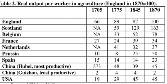
European urbanisation was accompanied by high and rising agricultural output per worker. By the beginning of the 18th century, agricultural yields were higher in Western Europe – and particularly England – than elsewhere in the world. Recent estimates of agricultural labour productivity (Brunt and Fidalgo, 2013) reveal massive differentials in output per agricultural worker around the world over the period 1700 to 1870, as reported in table 2.11
Table 2. Real output per worker in agriculture (England in 1870=100). 1705 1775 1845 1870 England 66 89 82 100 Scotland NA 59 129 163 Belgium NA 33 52 78 France 27 24 39 34 Netherlands NA 41 32 37 Prussia 10 8 25 50 Spain 15 14 14 23
China (Hubei, most productive) 273 48 39 45 China (Guizhou, least productive) 2 4 4 2
USA 19 29 45 45
Source: Brunt and Fidalgo (2013).
Table 2 highlights not only the high level of output per worker in England but also its strong growth during the 18th century, with an increase of 35% over the period 1705-1775. Alternative estimates for the growth in output per worker in English agriculture yield similar growth rates: for example, Clark (2002b, table 4) finds an increase in output per worker of 44% between the decades 1700-09 and 1770-79. Moreover, he documents that output per worker had already risen sharply in the 16th and 17th centuries, increasing fivefold between 1500 and 1650. Thus increasing agricultural productivity is an important candidate to be the trigger for the Industrial Revolution. The proposition that an agricultural revolution preceded the Industrial Revolution in England is hardly controversial – virtually every scholar agrees on this point – but the timing has been much debated. The earliest analysis (Ernle, 1912) suggested that the agricultural revolution was almost concurrent with the
11The sizes of the differentials may seem surprising. However, Maddison (2001) reports similar magnitudes for aggregate
labour productivity and, since agriculture was by far the largest sector in all economies throughout this period, aggregate and agricultural productivity are bound to be quite similar.
12
Industrial Revolution, with major changes occurring in agriculture after 1760. More recent research has almost universally favoured much earlier dates: classic contributions by Jones (1974) and Allen (1992) argued for the 17th century, whilst Kerridge (1967) maintained that it started in the late 16th century. Overton (1996) pushed back towards the late 18th century. In all cases, these dates precede the increase in output and productivity growth that is documented from 1800 onwards (Crafts, 2004), indicating that the timing of the agricultural revolution in England roughly matches the increase in urbanisation.
To sum up, Europe – especially England – exhibited high and growing urbanisation prior to the Industrial Revolution, while agriculture exhibited high and rising labour productivity. These stylized facts are consistent with our model’s prediction that a number of shocks that affected Europe resulted in an increase in urbanisation that predated the Industrial Revolution and contributed to knowledge generation. We formalize these possibilities in our model.
3. A model of urbanisation
We begin by setting out the components of the model. This section considers the determinants of urbanisation, taking manufacturing productivity as given. The endogenous evolution of manufacturing productivity is developed in section 4.
3.1 Population and preferences
We consider an overlapping-generations economy with workers and an elite. Agents live for two periods. At time t-1, 1 individuals are born who will be adult at t. Of these, are workers and belong to elite dynasties, comprising landlords and public officials, with . Workers have two possible occupations, farmer or manufacturer. We suppose that these occupations require agents to live either in the countryside or in cities, respectively, so agents’ location decision is bundled with their occupational choice.12 Young agents are born in the location chosen by their parents and make their occupation/location choice in the first period of their life; in the second period they work and have offspring. During the first period of their life, they may or may not acquire “ideas” that make them more productive, according to a process defined below.13
The elite receive rents from the farmers, to whom they let their land, as well as tax revenues
12 The simplifying assumption that manufacturing occurs only in cities is consistent with evidence indicating that only limited manufacturing production occurred outside cities in early modern times; see Coleman (1983).
13 The fact that individuals acquire skills when young, i.e. before they start working, fits well with a structure of apprenticeships, whereby young individuals chose their ‘trade’ at a relatively early age and acquired specific skills. See, for example, De la Croix et al. (2018).
1
13
that finance public offices. For simplicity, we suppose that the members of the elite are simultaneously landowners and public officials. This is most obviously true in England, where Parliament passed the Justices of the Peace Act in 1361 – creating the role of local magistrate, whose job was to administer local government and enforce the law but who remained unremunerated until 1835 (Magistrates Association, 2018). Since the magistrates’ position required education, free time and an incentive to manage local affairs (such as collecting local property taxes and disciplining paupers, as well as pursuing criminals), only the landed elites were qualified to fulfil this role.
We suppose that preferences are identical for all agents and take the form
, (1)
where and are, respectively, consumption of the agricultural and the manufactured good in the second period of life, and 1. This yields the demand functions
, (2a)
1 , (2b)
where is the income of the individual, and the prices of the agricultural and the manufactured good are, respectively, 1 and . The resulting indirect utility function can be expressed as
, (3)
where ≡ 1 .
3.2 Technology and factor payments
Agriculture
Agricultural output is produced with a constant returns to scale technology using labour and land, T,
, (4)
where denotes productivity in the agricultural sector, is agricultural labour, and 0 1. Our period of interest experienced significant improvements in agricultural technology, as documented by a large literature (for an overview, see Overton, 1996). Hence we assume that TFP grows at an exogenous rate g, so that = 1 .14
The wage in the agricultural sector is given by the marginal product of labour, that is,
(5)
14 It would be possible to make agricultural productivity endogenous, for example by assuming that a share of new ideas are applicable to agriculture rather than to manufacturing, which obviously would make agricultural productivity growth move together with manufacturing productivity growth. Since there is no evidence that this was the case, we chose to allow for exogenous agricultural productivity growth.
14
with the remaining income being paid to landowners as rents. We further suppose that agricultural workers are taxed at rate , so that the net income of farmers is given by 1 1
, where is the share of population employed in farming and ≡ / . Given the indirect utility function above, the utility of an individual working in the agricultural sector
is simply 1 .
Manufacturing
Manufacturing takes place in cities and the only input is labour. Manufacturing workers acquire ideas, denoted by i, when they are young according to a random learning process described below. We suppose that ideas, i.e. skills, are sector-specific, so individuals will not move when old.
The randomness of the learning process implies that ex ante identical individuals will eventually hold a different number of ideas. As we will detail below, at time t the maximum number of ideas available is given by t, with being the proportion of individuals that hold i ideas at t, and ∑ ∙ being the average number of ideas. We suppose that an artisan with i ideas produces 1 units of output. Summing across artisans, aggregate manufacturing output can be expressed as
, (6)
where is employment in manufacturing and ≡ 1 is average productivity in that sector, which depends on the average number of ideas that will be endogenously determined in section 4. The wage of a manufacturing worker with i ideas is simply given by 1 . Denote by the expected wage of working in manufacturing anticipated by the young. It is determined by the price and the (expected) distribution of ideas, that is, ∑ 1 , which can be expressed as and is independent of employment in the sector at time t.
Consider now the (indirect) expected utility of a worker living in the city and working in manufacturing. The linearity of equation (3) in income implies that expected utility depends only on the expected wage. Moreover, we suppose that there is a disutility associated with living in cities, denoted , so that expected utility can be expressed as that . This cost creates a wedge between rural and urban utilities that, in equilibrium, will result in higher wages in cities. Evidence of a gap between rural and urban wages is provided by Clark (2001), whose data show that an urban labourer earned around 20% more than a farm labourer in the mid-18th century. There are various possible justifications for the cost. Murphy, Shleifer and Vishny (1989) argue that manufacturing work itself generates a disutility for which workers have to be compensated, while Voigtläder and Voth (2013a) emphasize the health costs of living in cities, which is consistent with
15
falling average life expectancy in England through most of the 18th century (Davenport, 2015). Yet, technological progress is likely to have reduced it, due both to lower mortality rates stemming from improved medical know-how and reduced transportation costs due to the expansion of the canal system and railways.15 We hence allow the disutility cost to fall over time. In order to make this decline endogenous, we suppose that the cost falls with the level of technological know-how in manufacturing, that is, , where . is a decreasing function and bounded below at zero, lim
→ 0.
As well as being consistent with the existing literature, the presence of this cost is essential for our results. We will see below that increases in manufacturing productivity, , will reduce the relative price of manufactures. In the absence of , Cobb-Douglas preferences and technology would imply that the price reduction exactly offsets the increase in productivity, leaving and hence the manufacturing wage unchanged. The disutility creates a wedge in wages that implies that prices fall less than in its absence, thus resulting in an increase in the manufacturing wage.
Lastly, note that urban dwellers are assumed not to be taxed. This is a good approximation to the English context: the land tax was the main source of government revenue from the late 17th century to the First World War (typically generating around £2 million per annum, since the price level and land area were both approximately constant) and the agricultural tithe generated a similar figure; by contrast, the medieval shop tax had fallen into abeyance and urban producers remained virtually untaxed. Naturally, there were many minor changes in taxation over such a long period; an exhaustive history can be found in Dowell (1884).
3.3. Static equilibrium
Employment in agriculture and manufacturing
Workers can choose freely between agriculture and manufacturing, and will do so such that expected utility is equalized across the two sectors. The decision to migrate is taken by young individuals at time t-1 on the basis of their (rational) expectations of the income they would get at t in each of the two sectors. Note that some of the young in the city get ideas and others do not. This means that, ex
post, those in the city who got a below-average number of ideas will have lower utility than those in
agriculture. However, these individuals will not move into farming due to our assumption that skills
15Because of a lack of historical evidence on the cost of rural-urban migration, we turn to contemporary evidence. In rural
India, cash transfers that cover the cost of regular visits to the village of origin increase considerably the probability of migrating from a rural to an urban location (Lagakos et al., 2018), indicating that in low-income countries these costs still exist. In contrast, evidence on China shows that, in recent years, rural migrants permitted to move to urban locations are willing to forgo wage income in order to locate in larger cities with more amenities, implying that the cost has disappeared (Xing and Zhang, 2017).
16 are sector-specific and need to be acquired when young.
Equating to , and using the expressions above for wages in agriculture and manufacturing, we obtain the following relation between the price of manufactures and employment in agriculture
1 (7)
This equation implies a negative relationship between and , as a higher price will increase the manufacturing wage and result in migration away from farming. Higher productivity, , or higher taxation, i.e. a higher value of , result in a lower share of agricultural employment for any given price, since the former increases the manufacturing wage and the latter reduces the agricultural wage.
Goods market equilibrium
To obtain the goods market equilibrium, we need to consider the demands of workers and the elite. Worker demand is given by equations (2) above. The elite members receive both rents and tax revenue, i.e. all the output from the agricultural sector that is not kept by farmers, which is simply 1 1 . Since they have the same utility function as workers, their demands are also given by (2).16 Equating the supply and the demand for agricultural goods we have
1 1 1 . (8)
The first term on the right-hand side is the demand from the elite, followed by that from farmers and that from urban workers. Substituting for wages and output, this equation can be expressed as
, (9)
which gives the goods market equilibrium. This equation implies a positive relationship between agricultural employment and , for a given value of technology . The higher is employment in agriculture, the higher is agricultural output, which reduces the price of agricultural goods relative to manufactures.
The equilibrium allocation of labour
Equations (7) and (9) jointly determine agricultural prices and employment, so that the equilibrium allocation is determined by the system
16 We could allow the elite to consume imported ‘luxury goods’ as well as agricultural goods and manufactures, so that a fraction of output is not spent domestically. This would change slightly the expression for the relative price but would have no qualitative impact on our results.
17
1 (10a)
(10b) Since equation (10a) implies that is a decreasing function of , while equation (10b) yields an increasing function, there will be a unique equilibrium pair of price and employment for each value of
Bt, ∗ and ∗. Moreover, differentiating the implicit functions we have ∗ / 0, and
∗/ 0. That is, higher values of result in a lower ∗ as higher productivity in manufacturing
increases the wage in cities, inducing a shift of labour away from agriculture. This effect is partially offset by a price effect, since lower farming employment reduces agricultural output and drives up the relative price of agricultural goods. It is possible to show that the direct effect dominates and that increases, implying a higher urban wage. Agricultural employment is also affected by taxes and agricultural productivity, with the former reducing rural wages and hence inducing a flow of labour to cities. A higher value of (i.e. a larger ), shifts both functions as higher agricultural TFP increases the marginal physical product of labour in farming but reduces the price of agricultural goods, with the price effect dominating so that ∗ / 0. Lastly, a larger population (which reduces has the opposite impact, with the increase in the price of agricultural goods dominating and attracting more individuals into farming, thus raising ∗ . Note that this scale effect depends on the supply of land
being fixed, and that it can be offset by increases in either agricultural or manufacturing productivity.17 It is important to note at this point that the effect of productivity changes on the allocation of labour across sectors in dual economy models has been much debated; see Temple (2005) for a review. The predictions crucially depend on three aspects: the shape of the utility function, the factors used in production, and the potential wedges preventing wage equalization across sectors.18 In particular, the shape of the utility function determines the relative importance of income and substitution effects. When the substitution effect dominates, as is the case with CES utility, an increase in agricultural TFP and in manufacturing productivity have opposite effects on urbanisation, with the sign being determined by whether the elasticity of substitution is greater or smaller than one (i.e. by how prices change in response to productivity). If the income effect dominates, for example due to the existence
17 A possible interpretation is that scale effects are present only within a country, since the pressure on food demand as population increases can only be compensated by increases in productivity in either sector. In contrast, they do not appear across countries because population and land supply tend to be correlated.
18An example of the role of inputs is Hansen and Prescott (2002). In their model, agriculture uses land, labour and capital
but manufacturing only the last two factors. As a result, the manufacturing sector will not be operational for low levels of manufacturing productivity, and changes in productivity in either sector have no impact on agricultural employment.
18
of a minimum consumption requirement in agriculture, then increases in productivity in the agricultural sector raise demand for the manufacturing good more than for the agricultural one, inducing a flow of labour into cities. The income effect may also dominate in the presence of disutility costs associated with urban life, as is the case here. Note that for 0, equations (10) simplify to 1 1 1 . In that case, the allocation of labour is independent of the level of technology in either sector (as well as of the size of the population), the reason being that the price change exactly offsets the impact of any productivity change.
3.4. Per capita output
We are ultimately interested in the dynamics of per capita output. To be consistent with the evidence for the period of interest, the population is assumed to grow at a net rate of so that
1 , and we allow this rate to be endogenous. The way in which individuals choose their fertility as output and productivity change has been well studied (see, for example, Galor, 2011); we therefore abstract from fertility choices and simplify the population dynamics as much as possible, assuming that net population growth is an increasing function of per capita income, , i.e. .
Per capita real output in the economy is given by
, (11)
where equation (10b) has been used to substitute for the relative price and obtain the second equality. The first expression indicates that there are three effects of increased manufacturing productivity on aggregate output. Higher directly increases output, while it reduces the price of manufactures, making the price index, , fall which further increases real output. Lastly, the flow of labour away from agriculture and into the (now) more productive manufacturing sector provides an additional boost. Output is also affected by the dynamics of per capita productivity in farming, which are a combination of the (exogenous) productivity growth in agriculture and the (endogenous) rate of growth of the population. The former tends to increase and the latter to reduce output.
4. Cities and the transmission of ideas
The model so far has analysed the way in which a number of shocks to the agricultural sector can affect urbanisation and industrialization for a given level of manufacturing know-how. The next step in our analysis is to consider how urbanisation, in turn, has an impact on knowledge. This will result in a virtuous circle in which a shock increases urbanisation, which in turn raises productivity in manufacturing, thus inducing a further flow of labour into cities, and so on. Before we proceed, note
19
that a simple ‘black-box’ specification for knowledge creation – in which the latter is increasing in urbanisation – would deliver the feedback mechanism that we postulate. However, we are interested in understanding also what could drive the acceleration of growth observed in the data, as well as the gap between the paths of innovation and productivity. In order to do so, we now turn to the microfoundations of the knowledge generation process.
4.1 The creation and transmission of ideas
We suppose that, in each period of time, at most one idea can be invented following a process defined below. Ideas are ordered from i=1, 2, …t, according to the period in which they were invented, and an individual acquires knowledge sequentially, so that in order to hold idea i, he must also hold all ideas from 1 to i-1. Our two assumptions – bounded knowledge and sequentiality – are made for analytical tractability. The mechanism that we explore does not require either and we could, in principle, allow for an unbounded number of new ideas each period and non-sequential knowledge acquisition. However, the distribution of ideas would then have more parameters and following its evolution over time would become cumbersome.
Recall that is the probability that an individual has exactly i ideas at t and denote by the probability that an individual has at least i ideas at time t. Since there is a large number of individuals, these probabilities are, respectively, the fraction of the urban population that holds exactly
i ideas and that which holds at least i ideas. The sequentiality of ideas also implies that
1 .
There are two ways in which a young individual living in a city may increase his productivity. First, he may acquire existing ideas by meeting someone with those ideas. Second, young agents may also innovate and acquire one new idea during the period. We follow Glaeser (1999) and suppose that the number of meetings is a function of urban density. In particular, we suppose that the number of meetings is a strictly increasing function of the number of old individuals in the city, i.e. , with 0 0. That is, when nobody lives in cities, there will be no meetings. As in Glaeser (1999), we suppose that a young agent who meets someone with at least i ideas acquires these ideas with probability z. This means that the probability of acquiring at least i ideas in each meeting is , as
is the probability that the individual of the previous generation who has been met has at least those skills. If a young person has failed to learn something across all his meetings then he will not be able to imitate. The overall probability of not acquiring at least i ideas is therefore 1 , so the fraction of the population that has imitated at least i ideas can be expressed as
20
1 1 (12)
Additionally, an individual may come up with one new idea. Assuming that the probability that the individual does so after a particular meeting is , then the probability that he innovates during his youth is given by 1 1 . This particular assumption delivers the simplest possible setup in which innovation depends on meetings. Alternative assumptions could have been made about the probability of the individual innovating after a meeting – for example, making it depend on the average number of ideas held by the population. Such an assumption would have reinforced the dependence of innovation on past urbanisation. 19
The fraction of individuals that have at least i ideas is then given by those who imitated at least
i ideas plus those who imitated (i-1) ideas and then came up with an idea. That is,
1 , (13)
where 1 is the fraction of the population that has imitated exactly i-1 ideas at t+1, and
1 1 . (14)
Our framework has two implications for the innovation process. First, since agents can have at most one new idea during their youth, at any point in time t, there is an upper bound to the number of ideas held by an agent, and thus to knowledge – namely, t ideas. Second, although the probability of an individual innovating is independent of the distribution of knowledge in the population, the aggregate probability of a novel idea being invented is not. To understand this, note that – at the individual level – innovation may simply reinvent an existing idea, which will not add to the stock of knowledge; it is only those individuals who have imitated the existing t-1 ideas that may generate a novel idea, idea t. Consequently, the probability that a novel idea is invented in an economy with t-1 ideas is given by
1 , (15)
i.e. it is the product of the share of individuals that have imitated all existing knowledge and the probability that an individual innovates. Since the former depends on the distribution of ideas at t-1, so does the probability of an innovation occurring. may be zero, in which case idea t will not be invented, either because the urban population is zero ( =0) or because the fraction of the previous generation holding idea t-1 was so low that nobody has imitated it (i.e. 1 0 and
1 =0).20
19 This alternative specification is discussed in Appendix B.
20 Alternative formulations are possible that would not alter the basic mechanism. For example, there may be threshold effects so that an idea is added to the stock of knowledge only if is sufficiently large (see Appendix B).
21
In this context, there are two ways in which average productivity will grow: individuals copy the ideas of others that they meet – the diffusion of knowledge – and individuals observe the experiences of others and create new knowledge. The importance of these two aspects for the growth process is examined by Jovanovic and Rob (1989). In their setup, agents possess ideas of different ‘quality’. When two agents meet, there is both imitation by the less informed agent and invention of novel knowledge by both agents. We simplify their setup by separating the two processes.
We can now consider the distribution of the number of ideas. Recalling that is the probability that an individual has exactly i ideas at t, the average number of ideas at time t is simply
1 2 2 . . . 1 ∙ 1 ∙ . Moreover, since the fraction of the population with exactly i ideas can be written as 1 , and noting that
, we can write
1 2 . . . 1 ∑ (16)
and it follows that .
Using (13) and (14), the dynamic equation for the average number of ideas in the population can be rewritten as ∑ and, using the expressions above for and
, we have
1 1 ∑ 1 (17)
The first term captures the fact that a new idea is potentially invented each period. This aspect – the ‘creation of new ideas’ – is crucial because it will drive long-run growth. The second term captures the extent to which innovation is prevalent in the population. The term 1 is the fraction of the population that did not innovate, and depends negatively on urbanisation. The last term captures imitation and indicates that the share of individuals who did not imitate depends negatively on . Crucially, equation (17) implies that the current average number of ideas is increasing in the number of ideas held by the population last period and in the number of individuals living in cities.
4.2 The dynamics of urbanisation
Equations (10) and (17) – together with the labour market clearing condition, 1 , and the expressions for average manufacturing productivity, 1 – determine the dynamics of skills and urbanisation. The full dynamics of the model are then given by the following system:
) (i t
)
(
1 1 1 1P
i
I
t i t t
22 ∑ (E.1) 1 (E.2) 1 1 (E.3) 1 1 1 1 1 1 1 ∀ 1, … . , 1 (E.4) / (E.5) 1 (E.6) 1 (E.7)
The initial conditions of the economy are an initial population and level of agricultural productivity, and , and a distribution of ideas, . Average knowledge is given by (E.1); it depends on the distribution of ideas at t and in turn determines the cost of urban dwelling, as given by (E.2). Equation (E.3) has been obtained by combining equations (10a) and (10b), and it implicitly defines manufacturing employment at time t, , as a function of the average number of ideas (and of population and agricultural productivity). Manufacturing employment, or equivalently, the rate of urbanisation, together with the current distribution of ideas determine, by the set of equations (E.4), next period’s distribution of ideas. This distribution will in turn determine next period’s average productivity and the level of urbanisation, , and so on. The last three equations – (E.5) to (E.7) – give current output, as well as next period’s population and agricultural productivity.
To get an intuition for the dynamics of the model, let us consider a simplified version. Suppose that population, agricultural productivity, and the disutility of urban dwelling are simply constant parameters, i.e. , , , so that the dynamics of the model are given solely by equations (E.1), (E.3) and (E.4). Note that (E.3) defines the implicit function ; , , , , which is increasing in , i.e. 0. From equation (17) we can see that equation (E.1) implies that is increasing in since 1 1 and 1 1. It follows that / 0, implying that ideas grow over time; by equation (E.3), so does urbanisation.
23
Knowledge, defined as the number of ideas available in the economy, will grow without bound, inducing a flow of workers into the city. Equation (E.3) implies that, as → ∞, manufacturing employment tends to an upper bound given by
1. (18)
Both knowledge and productivity keep growing even if rural-urban migration stops. Knowledge grows because, as long as 0, a novel idea is invented in each period with positive probability. The arrival of a novel idea and its diffusion over the urban population imply that productivity keeps rising over time. Recall from equation (11) that there are three effects of increased manufacturing productivity on aggregate output: a direct productivity effect, the reduction in the relative price of manufactures, and the flow of labour away from agriculture. In the long run, the latter effect will be absent as urbanisation converges to , and output growth will be driven exclusively by the direct and the price effects of productivity growth.
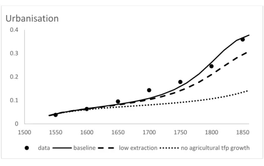
At this point, it is important to discuss two aspects. First, the key mechanism of the model is independent of our assumptions on population growth, agricultural productivity and change in the disutility, which are introduced to match the data. As discussed, the simpler model obtained when these are all constant generates the prediction that the feedback between urbanisation and innovation can generate a growth takeoff. Through numerical analysis of its dynamics,21 it is possible to show that – even in the absence of these three elements – the model also delivers an acceleration of urbanisation and growth. It cannot, however, match the historical data simply because agricultural productivity growth and population growth were substantial over our period of interest.
Second, let us consider what our setup implies compared to a ‘black-box’ knowledge generation function. A key result is that the rate of growth of productivity is lower than the rate of growth of knowledge because not all workers acquire the latest idea. In the early stages of development, when urbanisation is low, imitation is moderate and the gap between knowledge and productivity is large. As urbanisation increases, the gap between the two narrows due to a greater diffusion of knowledge. Secondly, depending on parameter values, we may observe an acceleration of productivity and urbanisation. If the probability of innovation is not too high, then most individuals increase their productivity through imitation. The nature of the imitation process implies that each generation has a higher probability of imitation than the previous one because there are more individuals holding i ideas than a period earlier, thus resulting in an acceleration of knowledge
24
diffusion, and consequently of output and urbanisation. Neither of these two features could be obtained with a simple ‘black-box’ specification for knowledge creation.
5. Revisiting the facts
The model in (E.1)-(E.3) has two key implications. First, it entails a feedback effect between innovation and urbanisation. It is possible to think of an initial situation in which this process is slow, resulting in negligible changes in urbanisation and knowledge, and in which anything that positively perturbs either the technology or the urbanisation rate sets a virtuous circle into motion that leads to the accumulation of knowledge and increasing living standards. Second, the model generates a wedge between manufacturing productivity and knowledge, which implies that – although the level of technology is growing rapidly – output is not because not enough individuals have learnt the new ideas. The next section presents numerical calibrations to examine in detail the implications of the model. But, before doing so, we consider how these two key results can help us interpret important features of the Industrial Revolution.
Ideally we would map the dynamic process of urbanization and subsequent economic growth across European countries. The current state of the data does not permit this, but we can offer some evidence from England. Bairoch’s city data enable us to calculate county-level urban populations in 1750 and 1800; we take county-level population data from the census (1801, 1851) and Wrigley (2009, for 1751). Since we do not have county-level output data – which would be ideal – we follow other authors (such as Dittmar and Meisenzahl, 2020) and use population growth as a metric for economic growth (see Appendix A for details on the data).22 In table 3, we regress county-level population growth between 1801 and 1851 on the urbanization rate in 1801. We also include county-level growth between 1751 and 1801 in order to control for any unobserved factors that may have made the county grow both in both periods. Between 1801 and 1851, we see faster growth in counties that were already more urbanized in 1801 (as well as those that were already growing faster in 1801). Even if not conclusive, the evidence is suggestive of the presence of the mechanism that we highlight, whereby urbanisation determines subsequent growth.
22 Of course, workers in the secondary sector earned significantly higher wages than those in the primary sector during industrialization. Since growth in population and secondary sector employment were strongly correlated (census data implies a correlation coefficient of 0.66), population growth is a downward-biased metric of income growth. In that sense, the coefficient obtained in our regressions underestimates the impact of urbanization on economic growth.
25
Table 3. Explaining county-level population growth in England, 1801-51. Dependent variable: Population growth
Constant 40.19† (9.49) Population growth, 1751-1801 0.67† (0.17) Urbanisation rate, 1801 0.85† (0.29) R-squared 0.53 N 42
†Denotes statistically significantly different from zero at the 1% confidence level. Standard errors in parenthesis.
Evidence from US development is also consistent with our urbanisation-industrialization-productivity growth sequencing. It makes little sense to consider the US economy as a single entity in the 19th century because some regions were heavily urbanised and industrialized before others had even experienced significant European settlement. For example, parts of the Northeast (Massachusetts, Rhode Island) had urbanisation rates above 50% by 1850 (US Census Bureau, 2012), while they were low in California before the Gold Rush of 1849. Regional patterns of urbanisation seem to have strongly impacted industrial development. For example, the first significant industry in the US was cotton manufacture and it is interesting that all the factories were founded in Massachusetts and Rhode Island – even though raw cotton was produced 1 000 miles further south. There are several reasons for this, but it has been argued that the business and technological know-how available in urban commercial centres (particularly Providence and Boston) were key elements (Nicholas and Guilford, 2014).
As we have argued above, a number of different factors can result in city growth, going from geography to plagues. Notably, Nunn and Qian (2011) argue that increases in agricultural productivity related to new crops were fundamental because they generated the potential to free labour from food production. Such a hypothesis fits well the case of England. A large literature has documented the fact that the agricultural revolution preceded the Industrial Revolution, yet the fact that the timing of the former roughly matches the increase in urbanisation in England is rarely discussed. Our model provides a possible explanation for the coevolution of these two variables.
Agricultural labour productivity may have increased because of exogenous technological shocks related to improved know-how or, as suggested by Nunn and Qian, to new crops. Our model proposes an additional source of increased productivity: agricultural extractions. The role of agricultural extractions as an additional shock during early modern times has received little attention
26
in the literature, yet it seems to us to have been particularly relevant in the case of England. High extractions from agriculture were the result of two phenomena. On the one hand, the established land property system in Northern Europe implied that a substantial amount of production went to the landowner, who was generally not the one who worked the land. On the other hand, agriculture was heavily taxed. In 17th and 18th century Europe, tax revenues were rising fast – particularly in England23 – and the main source of this tax revenue was the agricultural sector.24
Figure 4. Wages and rents plus taxes in agriculture in England (1775 English d).
Source: Authors’ calculations from Clark (2002b) and Brunt (2000); see text.
Figure 4 presents the evolution of indices for real wages, taxes and rents in the sector.25 English agricultural extractions had four components: land rents paid to landlords, the tithe paid to the church, local taxes (predominately the tax to support the poor), and the land tax paid by the occupier of the land to the central Government; see Appendix A for further discussion. The measure of extractions includes these four payments. Assuming that wages, taxes and rents exhausted the entire agricultural
23 See Karaman and Pamuk (2010), Dincecco (2011) and Voigtländer and Voth (2013b). Figure 5 in Karaman and Pamuk (2010) shows that, across Europe, per capita tax revenues were highest in England and the Dutch Republic in the 18th century; the was Netherlands also a highly urbanised country.
24 For an exhaustive account of the English case, see Dowell (1884).
25Clark (2002b; table 1) provides an index of real wages and the real value of taxes and rents. In order to get the level of
tax rates, we used data from Brunt (2000) on the value of output per worker and rents and taxes for 1775. Output was 975d/acre, which – with 20 acres per worker – yields an output per worker of 19 500d. This generates an extraction rate from gross output of 23% (=4 487/19 500) in 1775. We assume that total output is equal to wages plus extractions.