Coupled length scales in eroding landscapes

Coupled Length Scales in Eroding Landscapes

by

Kelvin Ka Wing Chan

Submitted to the Department of Earth, Atmospheric, and Planetary

Sciences

in partial fulfillment of the requirements for the degree of

Master of Science in Earth and Planetary Sciences

at the

MASSACHUSETTS INSTITUTE OF TECHNOLOGY

@

Massachusetts Institute

May 1999

of

Pinology 1999. All rights reserved.

Author ...

Department of Earth, Atmospheric, and Planetary Sciences

May 7, 1999

Certified by.

. ... . ... ...

Daniel H. Rothman

Professor

Thesis Supervisor

A ccepted by ...

Ronald G. Prinn

Department Head, Department of Earth, Atmospheric, and Planetary

Sciences

MASSACHUSETTS INSTITUTE 0L,

V----d

,,00.

Coupled Length Scales in Eroding Landscapes

by

Kelvin Ka Wing Chan

Submitted to the Department of Earth, Atmospheric, and Planetary Sciences on May 7, 1999, in partial fulfillment of the

requirements for the degree of

Master of Science in Earth and Planetary Sciences

Abstract

We propose a method to study natural topography by means of local transform. A nonlinear local transform A,[h(x)] of the elevation field h(x) is used to determine a director field of anisotropy a(x). The director field is directly related to local small-scale channel-like features. From study of the correlations of these with large-scale structure of drainage basins, characteristic coupling length large-scales are found which indicate an important breaking of scale invariance. We also show that these length scales are related to the average sizes of the individual drainage basins. Our study demonstrates one way in which landscape patterns of unknown origin may be quantitatively analyzed to determine the kind of mechanisms that have eroded them. Thesis Supervisor: Daniel H. Rothman

Acknowledgments

Zeroth, my thanks go to our Almighty Boss above, who kindly created us and this universe (which is so complicated and interesting that we shall never be bored). Without Him, nothing ever is possible.

First, I thanked my parents, Kai Ping and Wai Chi Chan. They obviously had spent many hours of their lives to make sure that I am doing ok and lead a balanced life style (which I find it very difficult to achieve at MIT). They have supported me both financially and psychologically to get through my undergraduate years and now my graduate years. I also thanked my brother, Kelly Chan, for his kind and timely reminder of the sanitary condition of our bathroom and kitchen.

At MIT, my warmest thanks go to my advisor Dan Rothman, who introduced and initiated me into the world of complex and nonlinear dynamical systems. Without his many hours of advising and humorous remarks, this thesis will never be possible.

I also thanked my co-advisor John Grotzinger, who had provided me the opportunity

and funding to work on an interesting geological problem with some astrobiological relevance. He also invited me to join his geological field trips in NWT Canada (sum-mer 1996) and New Mexico (spring 1999), the two most unique and thrilling academic experience I ever had and unlikely to be duplicated elsewhere. I also thanked Yen Feder and Andrea Rinaldo for their helpful discussions and for giving me important insights into my research.

I was also fortunate to have support and companies from friends: Ernie Yeh,

Albert To, Edwin Cheung, Connie Cheng, Edward Wong, Oliver Yip, Agnes Wang, Jimmy Wong, KM Lau, Philip Lo, Oliver Yip, Agnes Wang, Jimmy Wong, KM Lau, James Mak, Wing Wah and Dorcas Sung, Zachary Lee, (please forgive me if I forgot to mention names which you think I should) and many other brothers and sisters at the Hong Kong Student Bible Study and Daniel Fellowship, whom I had shared my stresses and joys with. Millions of thanks go to you all.

Last but not least, my gratitude extends to my colleagues and friends at EAPS: Peter Dodds, Romu Pastor-Satorras, Olav van Genabeek, and Wesley Watters who

had all helped enormously in my research and course works. I also thank Joshua Weitz and Davide Stelitano, who sometimes kept me company late at night at Bldg 54.

Contents

1 Introduction 12

2 The method 15

2.1 Apparent dip direction and anisotropy in fluvial erosion . . . . 15

2.2 Wave packet and local transformations . . . . 17

2.3 Correlation between small and large scale structures . . . . 20

2.4 Note on computing a(x; fc)

. . . .

22

2.5 Tests on isotropic synthetic topography . . . . 23

2.6 Tests on a synthetic inclined anisotropic surface . . . . 24

2.7 Some details on artefacts due to discretization, finite domain, etc . 26 3 Results 29 3.1 Results from empirical studies . . . . 29

4 River Drainage Basins 37 4.1 Fractal river basins and networks . . . . 37

4.2 Total contributing area Ai . . . . 38

5 Relocalization of Correlation Functions 44 5.1 Fluvial erosion processes . . . . 44

5.2 Coupling total contributing area Ai to the slope s . . . . 45

5.3 Results from empirical study . . . . 47

A Wave packet

B Error Analysis

B.1 Error in assuming uniform grid .... ...

B.2 Error in assuming the shortest distance between two points lies along the latitude . . . .

C Measuring Local Anisotropy of Plane Waves and Band Pattern D Data Exposition E Fractures 56 59 59 60 63 65 71

List of Figures

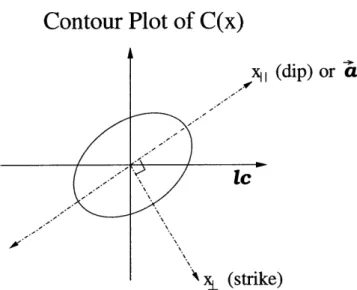
1-1 An inclined plane possesses two directions. x (tip) is in the direction of dominant flow and xz (strike) is the direction perpendicular to this. 12 2-1 Contour plot of C(x) assuming validity of linear theory and x < L

where L is the system size . . . . 15

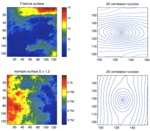
2-2 Contours of C(x) for a fracture surface and a synthetic isotropic self-affine surface of D ~ 1.2. Note that at small x (near the center), the contour is elliptical for the fracture surface (which is known to be anisotropic) but circular for the isotropic surface. . . . . 16

2-3 Wave packet W(x/c,

#)

with the extent of the packet fc = 4o-. Note that

#

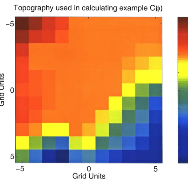
is the orientation of the plane wave in the planar direction (the plane perpendicular to the page). . . . . 17

2-4 Example topography for calculating C(#) . . . . 19

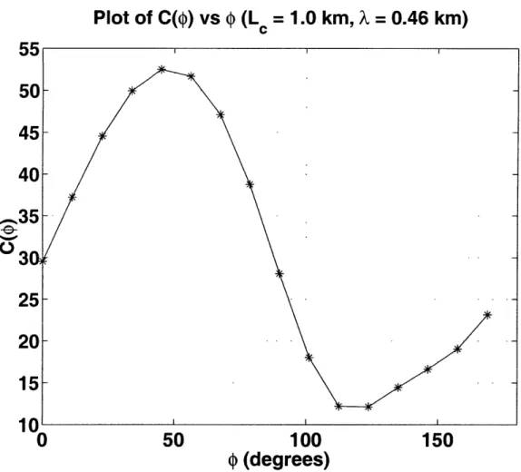
2-5 Plot of C(#) computed for the topography shown in Fig. 2-4 . . . . . 20

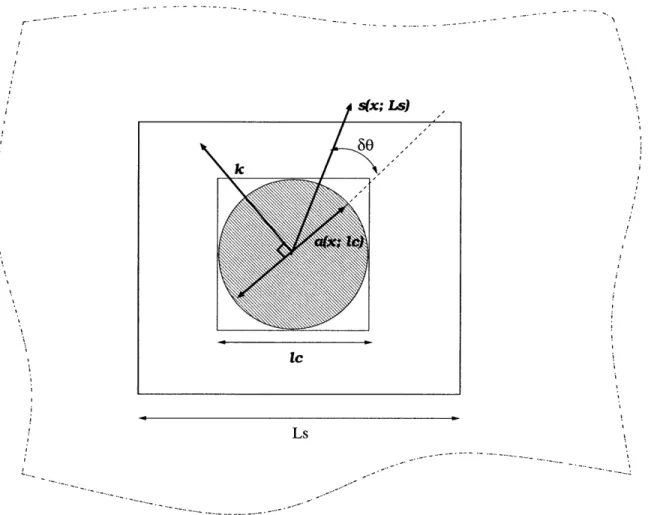
2-6 Diagram showing boxes (with sizes fc and L,) within which a and s are computed. The angular separation between them is labelled 60. Note that a is defined to be perpendicular to the local dominant wavevector k and a is indistinguishable from -a. . . . . 21

2-7 ... ... ... 24

2-8 For synthetic isotropic self-affine surface with D = 2.1 . . . . 25

2-9 For synthetic isotropic self-affine surface with D = 2.1 . . . . 26

2-11 For a synthetic inclined anisotropic surface. Note: dip is in the direc-tion of steepest descent and strike is the direcdirec-tion parallel to it and that C(xL) > x1) . - - . . .. . . . - - - ... - 27

2-12. ... ... ... 28

3-1 Topography used in this study. Data is obtained from USGS 1-degree

DEM which ranges from 121'W/390N to 120"W/38"N. . . . . 31 3-2 Anisotropic director field for the topography (121 0W/390N to 1200W/380N). 32 3-3 The average cosine square of the angular separation of a and s vs

relative scales L,/4c. This shows that the apparent dip direction a at small scale fc = 1 km is most strongly correlated with the slope s = (Vh) measured at L* - 10 km >

4c.

. . . . 33 3-4 This shows the distribution of the angular difference 60 between the

apparent dip direction a measured at small scale

4c

= 1 km and the slope s measured at large scale L* = 10 km. It indicates that the most

probable 60 ~ 00. . . . . 34

3-5 Plotting (cos2 _{60) for various fes. L* is the length scale at which the}

correlation becomes optimum. Here we see that L* ~ 8-15 km for all

values of

4c.

. . . .

35

3-6 A plot of the optimal large scale L* vs log

4c

(Log of length scale at which a is measured). This shows approximately L* ~ log

4c

for large

4c.

36

4-1 Total contributing area at a point, which is related to the characteristic area of the basin. . . . . 39

4-2 Figure showing the coarse graining scheme. At each step, the new grid point is taken to be the average of the neighboring cluster of 4 grid points forming the square . . . . 40 4-3 The study of the exceedence probability distribution of total

contribut-ing (drainage) Ai under different coarse graincontribut-ing scales b. . . . . 41 4-4 Study of the dependence of (A)1/ 2 _{on coarse graining. . . . . 42}

4-5 A comparison between L* and (A) 1/2 measured at different length

scales. The topography is the same as the one used in the previous

analysis. . . . . 43

4-6 L* is related to the length scale of the average drainage area (A)'/ 2, or the average basin size. . . . . 43

5-1 A, is a global function in the sense that it depends on the structure of h(x) within the basin. A set of Ai near the outlet therefore contain informations about the large scale topographical structures covering the basin that drains into it. . . . . 46

5-2 Results for 121'W/390N to 120"W/380N, n = 1 in all of the above. . . 48

5-3 Results for 121"W/390N to 120'W/38"N, n = 1 in all of the above (P art 1). . . . . 49

5-4 Results for 121"W/390N to 120"W/38"N, n = 1 and fc = 8.44 km (P art 2). . . . . 50

5-5 Showing that L*/ ~ 1 at m = 3 and n = 1 . . . . 51

5-6 Showing that L* does not depend very much on fc (shown for m = 3). 51 5-7 W (L,) depend on m . . . . 52

5-8 W and L, can be rescaled by m3 and m' to collapse on top of each other. The deviation at large Ls is finite size effect. . . . . 52

5-9 L* - m ~03 for

4c

= 3.8 km . . . . 53

A-1 Dependence of

(lal)

on

4c

with plane waves of different A. It shows that for c/A > 10, the effect due to discretization, finite cutoff inte-gration, and finite size effect of plane wave becomes insignificant and

(lal)

becomes independent of c for a fixed plane wave of k' = k. . . . 58

B-1 ... ... 61

B-2 ... ... 61

B-3 ... ... 62

C-2 Figures showing the local anisotropic director field for a waves . . . . . . ... Results for 1210W/390N to 120"W/380N, m = 0 . . . Results for 1210W/390N to 1200W/380N, m = 1 . . . Results for 121"W/390N to 1200W/380N, m = 2 . . . Results for 121"W/390N to 120"W/380N, m = 3 . . . Results for 1210W/390N to 120"W/38"N, m = 4 . . .

-+ direction of crack propagation . . . .

Plots of W as a function of L, and fc for different sets Results for fracture topography . . . .

set of plane D-1 D-2 D-3 D-4 D-5 E-1 E-2 E-3 of m and n..

Chapter 1

Introduction

xII

Figure 1-1: An inclined plane possesses two directions. x1 (tip) is in the direction of dominant flow and x1 (strike) is the direction perpendicular to this.

Natural landscapes can be influenced by multitude of factors that may be physical, chemical, or biological in origins. Geomorphology principally concerns itself with the study of surface features and structures influenced by exogenic processes (those originated from outside the solid earth) [2]. These included fluvial erosion, glacial and periglacial erosion, avalanches, aquatic effects, aeolian erosion (wind and sand movement), biological activities (vegetation), etc. But in general, at relatively large scales, geomorphology is dominated by tectonic motion (endogenic processes) while at shorter scales, surficial erosion plays an important role.

Despite the diversity of processes and highly heterogenuous geological conditions (in time and space), landscapes generally erode in part due to material transport [2] and the resultant shearing stresses imposed by the flow. However, the exact for-mulation of a theory for fluvial erosion is not known. It is well known that

natu-ral landscapes possess fractal (or self-affine) geometry

[1,

3, 4] and geomophological

complexity can be observed over many length scales. The underlying theory must therefore account for all these observations at the appropriate scales. This concept of self-affinity of natural landscapes has provoked the suggestion that erosion follows mechanisms similar to a wide variety of surface growth problems [5].

More recent studies of fractal nature and minimization principle of river basins and networks had involved concepts and ideas known as optimal channel networks and self-organized criticality [7, 8]. This indicates that careful study of macroscopic

patterns can yield fundamental insights into the microscopic basic mechanisms [11]. Therefore, a more detailed and physically motivated quantitative study of topography may be needed to yield information about features unique to fluvial erosion.

It may be true that models of fluvial erosion involve some common general con-siderations such as symmetries, range of interactions, nonlinearity, conservation laws, etc., which do not all depend on system details and give rise to universal features in pattern formation [11]. But quantitative features special to eroded landscapes must be studied if one wants to gain access to the detailed dynamics of landscape evolution. Recent observation and theoretical works [6] show that statistical properties of landscape can be influenced by the dominant direction of flow on its surface. Specif-ically, they compute the height-height correlation function C(r) = (|h(x + r)

-h(x) 12)1/2_{. The most ubiquitous and consistent observation is that C(x±)}

> C(x1)

where xl1 is in the direction of the flow (dip) and xi is orthogonal (strike) to it. See

Fig. 1-1. For self-affine surfaces, C(x) - x'. Physically, this corresponds to the

observation that topography is rougher transverse to the flow than in the direction parallel to the flow. A nonlinear model was proposed resulting in a stochastic PDE of growth which predicts different roughness exponents all and a1 for the two directions. This has been observed in a submarine canyon off the coast of Oregon [6]. For real landscapes in general (rather than an incline with an obvious downflow direction), the directions of main flow will depend on the topographic structure observed at dif-ferent scales. Furthermore, the self-affinity and/or geometric complexity of natural landscapes imply that the local statistical anisotropy be also scale-dependent.

Inspired by these simple observations and motivated by the need of a quantitative study of eroded topography, we raise some important questions concerning natural landscapes: How does local anisotropic structure (related to local channelization) cor-relates with the general topographic features (related to relief structures of drainage basins)? At what length scales? Are there optimum scales at which they become most strongly correlated? If such scales do exist, what are their physical interpretations and how do they relate to the physical topography? Conceptually, the two aspects (anisotropy and topographic structure) involved are coupled via fluvial erosion and the preferred directions of material transport along the surface. This indicates that the questions we posed are relevant investigations of the general characters of fluvial erosion of natural landscapes. On the other hand, the nonlinear nature of surficial growth is likely to be a consequence of the interactions of processes operating at differ-ent length (or time) scales. These couplings of length scales may manifest themselves in the correlation between large and small scale features of the topography.

This prompts us to study empirically the correlation between surficial anisotropy (local channels) and topographic structures (drainage basins). We propose a way of studying this surficial anisotropic structure using local transforms and correlation functions. The method involved is largely inspired by works on the analysis of pattern-forming systems [9, 10]. In the following chapters, we first introduce the method we use and some assumptions we make. We then present results from the study of to-pography which ranges from the western flank of the Sierra Nevada mountains to the eastern edge of the Central Valley. This leads to the discussion of how our findings connect with some important results in geomorphology concerning erosion, total con-tributing area, and local slope. Finally, we discuss the various physical implications and interpretations of the empirical results have on some general characteristics of fluvial erosion.

Chapter 2

The method

2.1

Apparent dip direction and anisotropy in

flu-vial erosion

Contour Plot of C(x)

x1 (dip) or a

\ xL (strike)

Figure 2-1: Contour plot of C(x) assuming validity of linear theory and x < L where

L is the system size

Since a preferred direction of flow leaves a statistical signature in the height-height correlation function C(x) = (|h(x'+x) - h(x')|2) . It is in principle possible to infer

the original direction of dominant flow by studying the structure of C(x) alone. In the linear theory and the limit x < L where L is the system size, one expects elliptic

of C(x) for a fracture surface (after L6pez and Schmittbuhl) and a synthetic isotropic self-affine surface of fractal dimension 1.2 in Fig. 2-2. Note that at small x, the contour is elliptical for the fracture surface (which is known to be anisotropic) but circular for the isotropic surface.

Fracture surface 2D correlation function

15 20 150 14 40 140 60 13 130 80 12 120 100 ₁₁₀ 11 120 100 20 40 60 80 100 120 100 120 140 160

Isotropic surface D = 1.2 2D correlation function

20 0.76 150 40 0.758 140 60 130 0.756 80 120 0.754 00 ₁₁₀ 120 0.752 100 20 40 60 80 100 120 100 120 140

Figure 2-2: Contours of C(x) for a fracture surface and a synthetic isotropic self-affine surface of D - 1.2. Note that at small _{x (near the center), the contour is elliptical for}

the fracture surface (which is known to be anisotropic) but circular for the isotropic surface.

When applied to natural topography, from the semi-major and semi-minor axes of the ellipse, one can deduce an apparent dip direction. This can also be regarded as the local anisotropic director field a(x). A director is a vector with angular orientation but no direction: a is indistinguishable from -a. One may represent it by a straight line, but no arrow to indicate the direction. This is the conceptual justification of an

apparent dip direction. But we shall deduce this through another method. This is

largely inspired by recent applications of wavelet transforms in the analysis of pattern formation [9].

2.2

Wave packet and local transformations

We first define the kernel or the analyzing function of our local transform (with a

wavenumber

|kI):

(2.1)

W (x, #)f=2

where

ko= -(cos

#,

sin

#),

0 < < 27r

A (2.2)

g(y) - exp(-8y2).

This is equivalent to a plane wave with an amplitude modulated by a Gaussian envelope with standard deviation o- =/4. See Fig. 2-3. Then, we correlate the

2a

Figure 2-3: Wave packet W(x/fc,

#)

with the extent of the packet fc = 4o-. Note that

#

is the orientation of the plane wave in the planar direction (the plane perpendicular to the page).

e

---iko -x -fc

wave packet with local topography h(x) within a box size of

4c.

C(x, #;

c)

J

dx'

W e(x'

-

x,

#) h(x')

(2.3)

Jix'-xi<fc/2

For a chosen location x and |k! (or A), C(x,

#;

4)

computed at scale fc only depends on

#.

For anisotropic surface, C(#) should be predominantly ir-periodic in

#,

at each location x. See Fig. 2-5 for an example of C(#) calculated from the topography shown in Fig. 2-4. Then, the angular orientation of a(x) is defined to be perpendicular to the phase of the ir-periodic part of C(#) and is related to the local dominant wavevector k(x) of the topography. To obtain the phase of the ir-periodic part, we compute:

Z = e- 2_{0 C(#) d#. (2.4)}

0r

with a(x) derived from Z by:

a(x) = [-j(Z), R(Z)] and a(x) I k(x) (2.5)

or simply let jai =

IZI

with the orientation of a orthogonal to that of Z.

Formally, this can be conceptualized as a nonlinear transform Af[h(x)] of the eleva-tion h(x) to obtain a new field a(x;

4c)

for a particular choice of wavelength A of the wave packet (used in the transformation). Note that this is defined at a length scale

fc.

To obtain a measure for large scale topographic structures, we compute the "real" slope s(x; L,) at location x averaged over a length scale L,:

-5

Topography used in calculating example C()

630 620 610

I

600

-5

0

5

Grid Units

Figure 2-4: Example topography for calculating C(#) The average is taken as followed:

(Vh(x))L, = g(X LX, fIx-xILs/2 dxlg(xjx) lVh(x)I -xI L,/2 dx'g( X) =1 exp 8 L

We expect the local dominant (preferred) direction of flow to be related to s(x; L,).

590 580 570 560 550 where (2.7) (2.8)

Plot of C($) vs

$

(Le = 1.0 km, X = 0.46 km)

55

,35

10'

'

'

0

50

100

150

$

(degrees)

Figure 2-5: Plot of C(#) computed for the topography shown in Fig. 2-4

2.3

Correlation between small and large scale

struc-tures

To answer our previous question about the correlation between small and large scale structures, we need to examine the correlation between a and s computed at different scales. Specifically, we want to know if a(x; fc) is parallel (or anti-parallel) to s(x; L,),

and if so, at what relative scales? At each point in space, we compute the angular difference between the two vectors:

60(x; LS, fc) = cos- {a(x;ec> s(x;L,) (2.9)

Figure 2-6: Diagram showing boxes (with sizes fc and L,) within which a and s are computed. The angular separation between them is labelled 60. Note that a is defined to be perpendicular to the local dominant wavevector k and a is indistinguishable from -a.

See Fig. 2-6 for a clarification. From this, we can calculate various statistics such as, Prob(69), (60), ((69)2), (cos2_{(60)), etc. (2.10)}

as a function of Ec and L, (and A), where () is an average over the spatial domain of interest.

We pay special attention to the following statistics (or correlation function) in our analysis:

which is the average cosine squared of the angular separation of a and s, and

W {|a.s|2₎

(a|

2_|s|2 cos2 60) (|a121s|2) _(|a121s12)

which is the weighted average cosine squared of the angular separation by the

mag-nitude |a|2 and fs|2_.

2.4

Note on computing a(x; fc)

It is known in signal processing that if a time series has an unambiguous linear trend, the resulting power spectrum will be a power law decay of S(k) - k-2. This can be easily seen when we consider the Fourier coefficients in the following function:

{

kx, for

0< x <a

0, otherwise.

where k and a are constants. The magnitude of the Fourier coefficients will decay

as - 1/n 2 _{with higher harmonics parameterized by increasing n. A signal with a}

linear trend can be regarded as the sum of a function like

f

(x) and a part without

a linear trend (which contains the small scale structures of the original signal). As a result, the statistics of the small scale structures and fluctuations revealed by the power spectrum (or correlation analysis) can be obscured by the contribution from the overall trend. This will not be desirable in studying local anisotropy. To remedy this, we detrend locally our topography by subtracting from it the best fitting plane:

minx 2 _{= [h(r) - f (r; a, b)]}2_{, where f (r; a, b) = ax + by + c.}

{a,b} _rER

h'(r) = h(r) - f (r; a, b). (2.11)

2.5

Tests on isotropic synthetic topography

As a control, we would like to apply our methodology in correlating local anisotropy a with local slope s to a synthetic isotropic self-affine topography. The basic technique to generate such topography is to convolve Gaussian noise q(x) with a kernel G(x) such that the resulting signal possesses an algebraic power spectrum. ie. h(x)

E, G(x - x')(x') with h(k) ~ k-. We follow the algorithm indicated by [12]:

1) Generate an N x N square grid consisting of N2 _{equally spaced points of Guassian}

random variables rmn.

2) A two-dimensional discrete Fourier transform is taken:

N-1 N-1 _{- .7}

=st

= (1/N)

2

Sm

S

rlnnexp

[

(sn + tm)]

n=O m=O

generating an N x N array of complex coefficients 4_st.

3) A fractal dimension D is specified with the corresponding exponent

#

given by

D = (7 -

#)/2.

The Fourier coefficients are then filtered as followed:

Hst = st/kf /2

4) An inverse two-dimensional Fourier transform is performed to obtain h(x). The topography used in the testing is shown in Fig. 2-7. We choose a fractal dimension of about 2.1.

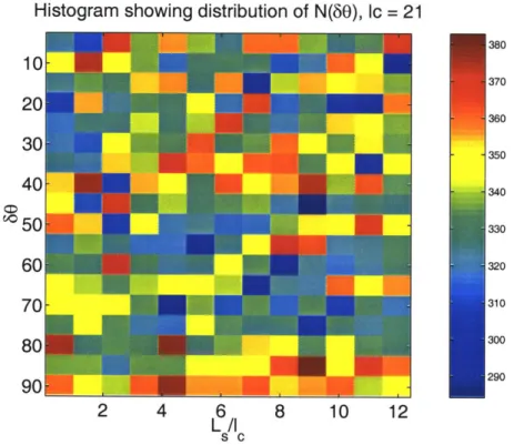
Since this is isotropic, we expect to see no correlation of a and s. As suspected, we discover that the angular separation between a and s is randomly distributed with no correlation at all scales L. with which we compute our s. Fig. 2-8 is a histogram showing the distribution of 60 with different Ls, but with fc fixed at 21 grid units.

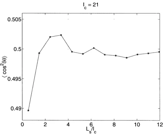
Fig. 2-9 shows how (cos 260) varies with L., again with fc fixed at 21 grid units.

Self-affine surface with D = 2.1 0.768 100 s 0.764 300 0.762 400 *-0.76 700 0.758 800 0.752 0.754 900 _0.752 0.748 1000 200 400 600 800 1000 Figure 2-7:

(cos 2_{60) fluctuates around 0.5, indicating a random distribution over all possible}

angles.

This result indicates that any deviation away from uniform distribution of 60 is significant and comes from the genuine anisotropic nature of the surface.

2.6

Tests on a synthetic inclined anisotropic

sur-face

As a further understanding of the characteristics of the correlation between a and s, we apply the method to an "ideal" slope. This is an inclined anisotropic surface with

C(x1) > C(xjj). See Fig. 1-1. The algorithm for generating this surface is exactly

the same as for the isotropic case, except that in filtering the Fourier coefficients, the following is done:

Hst= fst|(k2 + Ak 2)!/

Histogram showing distribution of N(860), Ic = 21 380 10 370 20 360 333 S50 330 60 320 70 310 300 80 90290 2 4 6 8 10 12 L /I S C

Figure 2-8: For synthetic isotropic self-affine surface with D = 2.1

Fig. 2-10 shows the inclined surface we used. It is made smoother in the dip (xI1)

direction than the strike (xz) direction. This is the prediction of the linear theory of stochastic anisotropic diffusion and it is almost always observed in real topography. To check that the topography we generated is anisotropic, we calculate its height-height correlation function C(x) in both the dip and strike direction. The result is shown in Fig. 2-11.

Notice that C(xz) > C(x). We would like to see how a correlates with s. We

apply our method of extracting a from local transforms, and study how (cos 260)

changes with L,. The result is presented in Fig. 2-12. We can clearly see that a measured at fc = _{21 becomes more and more correlated with s measured at larger} and larger L,. The simplest explanation is that the anisotropic orientation has been set to line up with the direction of the inclined plane (dip). When you measure s at a scale smaller than the system size, in addition to the global slope direction, you will also pick up local fluctuations. The smaller the scale with which you measure your slope, the more significant the local fluctuations become. Therefore, the correlations

1 =21 C 0.505-0.5 CMJ U, 0 0.495- 0.49-0 2 4 6 8 10 12 L /I S C

Figure 2-9: For synthetic isotropic self-affine surface with D = 2.1 will not be high when L, is much smaller than the system size.

This exercise has shown empirically that our method of local transforms in mea-suring local anisotropy a and local slope s can indeed yield useful information about how one correlates with the other at different scales.

See Appendix C for the local anisotropy director field measured for a set of plane waves and a pattern of stripes and bands.

2.7

_{Some details on artefacts due to discretization,}

finite domain, etc

It can be shown that the various numerical artefacts due to discretization, finite limit of integration (in performing local transforms), etc., are remedied when c/A > 10 is

"Ideal slope" 200 400 600 800 1000 Figure 2-10: Correlation function C(x) *q -.... ...S trike... qDip 10 1 102 10

Figure 2-11: For a synthetic inclined anisotropic surface. Note: dip is in the direction of steepest descent and strike is the direction parallel to it and that C(xi) > C(x)

100 200 300 400 500 600 700 800 900 1000

30

100 10 10 0

"Ideal slope", I = 21 6 L /l S C Figure 2-12: ,~0.7 C) 0 0.

Chapter 3

Results

3.1

Results from empirical studies

Topographical data is obtained from the USGS online database. The 1-degree Digital Elevation Models (DEM) is used which provides coverage in 1- by 1- degree blocks. It consists of a regular array of elevations referenced horizontally on the geographic (latitude/longitude) coordinate system of the World Geodetic System 1972 Datum

(WSG 72) or the World Geodetic System of 1984 (WGS 84). There are 1200x 1200

sample elevations in each block. We use linear interpolation to obtain an evenly spaced square grid of data in rectangular coordinate. In projecting the data from spherical to rectangular coordinate, we commit systematic errors which we can show to be negligible for our purposes. Details can be found in Appendix B.

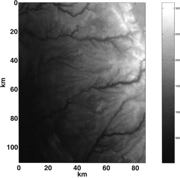
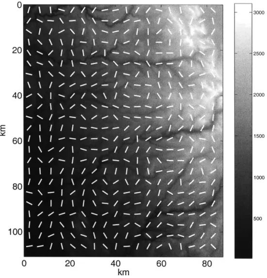
We study a piece of topography that ranges from 384-39' north latitude and 1204-121" west longitude, a rectangular area whose dimensions are roughly 100 km on a side, with a resolution of approximately 90 m. This area, entirely contained within California, ranges from the western flank of the Sierra Nevada mountains to the eastern edge of the Central Valley. (Fig. 3-1). Our area of interest contains a drainage basin with an unambiguous dominant slope (or direction of flow), and network of rivers can be seen to flow downhill in mostly one direction. A wide range of erosive features exist, including those of glacial, fluvial, and alluvial origin. The field of anisotropic director field is shown in Fig. 3-2. We compute (cos2

different relative scale L,/Ec at

4c

= 1.0 km. The result is shown in Fig. 3-3. We discover that a measured at small scale f4 = _{1.0 km is most strongly correlated with} the slope s measured at L, - 10 km >

4c.

To convince ourselves that for L, in this vicinity, a and s are most probably lined up, we examine the distribution of 60 for the case of

4c

= 1 km and L* = _{10 km. See Fig. 3-4. This clearly indicates that the} most probable 60 - 00. _{This shows anisotropy measured at small scale f4 is most}

correlated with large scale topographic features at L*. In addition, we also examine a synthetic isotropic landscape with cross-section fractal dimension of df = 1.2. We find no such correlation and 60 is distributed at random as expected.

Finally, we examine the dependence of (cos 2 _{60) on L, for different f. The result}

is shown in Fig. 3-5. Note that some of the curves have been displaced vertically to allow a clear comparison. It is observed from all the plots that local anisotropies cal-culated at scale

4e

are always most strongly correlated with local slope (or direction of dominant flow) measured at a larger scale L,. We define this "optimum" length scale as L*. On closer examination of Fig. 3-5, we discover that L* increases monotonically with

4.

We make a plot showing this in Fig. 3-6. It is found that when fitted to a power law, it has a very weak exponent which leads us to postulate L* - log

4.

This

may be related to the fact that surficial erosion operates over a range of length scales rather than a distinct characteristic scale.

In a more general framework, the local slope (dominant direction of flow) can be regarded as a "stress" on the system and the local anisotropy as the "response" to this directional "stress". The results show that in the case of natural landscapes, the "response" is always correlated with a certain overall "stress" defined over a large scale.

However, the physical interpretation and significance of L* and its relation to the local features of topography need to be examined more closely. This will be elucidated in the next chapter. Future investigation using this method can also provide a chance to study the "up-down" (a)symmetry of fluvial erosion, ie. to investigate if erosion at a point on a hillslope is more correlated with processes in the upstream or the downstream direction.

3000

20

-2500

E

40

2000 1500

60

1000

80

500 100

0

20

40

60

80

km

Figure 3-1: Topography used in this study. Data is obtained from USGS 1-degree DEM which ranges from 121"W/39"N to 120"W/38"N.

Willi

7

it'.-....-

i\--u-IUUEEEIEIEEIEEM

IEh.IIIEImE

El.

L

-NJN

40

km

60 80

Figure 3-2: Anisotropic director field for the topography (121"W/39"N to

120"W/380N). - -o3000 ou 80 100 A 20 i \ l -- - -- -'01 -\ 0,/- \ - -- / \ /

I

--- / --- - | \

\0--0.55F

0.5

0c.45

CD

ci)

0

0.4

0.35

0.30

0

5

10

15

20

25

L /L

_{S C}

Figure 3-3: The average cosine square of the angular separation of a and s vs relative scales L,fc. This shows that the apparent dip direction a at small scale fc = 1 km

For L

=

1.0 km,

(X =

0.46 km)

20

40

60

80

60 (degrees)

Figure 3-4: This shows the distribution of the angular difference 60 between the apparent dip direction a measured at small scale fc = 1 km and the slope s measured at large scale L* = 10 km. It indicates that the most probable 69 ~ 00.

0 07'

Cn .

0

20.04

CD

£0.05

LL

N

0.02

C-E

S0.01

z

0'L

0

F

(X = 0.46 km) Le (km) +I-* 1.0 G-0 2.9 x--x 4.7 +-+ 6.6 0-4 8.4 10 15 L (km) 20 25

Figure 3-5: Plotting (cos 2 ₅₉₎

correlation becomes optimum.

for various Ecs. L* is Here we see that L*

the length scale at which the

8-15 km for all values of Ec

0.8F 0.7h 0.6 k CO) 0 0.5k 0.4k 0.3[ 0

16

15-

14-

p13-

11-

10-9'

0

0.2

0.4

0.L(

p

0.8

1

log

Lc

(k

Figure 3-6: A plot of the optimal large scale L* vs log fc (Log of length scale at which a is measured). This shows approximately L* - log fc for large fc.

Chapter 4

River Drainage Basins

4.1

Fractal river basins and networks

When water flows across a landscape from the drainage source to outlet, it does so in channelized networks. With the availability of digital elevation maps (DEM), it becomes possible to extract the drainage pattern of a large river network over an extended area (typically in the order of hundreds to thousands of kilometres). This enables a study of the structure and scaling properties of such fields and networks. The most striking feature of such networks is that they are fractal in nature [7]. It is very difficult to tell the difference between the Amazon and the little creek in your backyard without a scale bar. The most ubiquitous result is the power law distribution of the total contributing (drainage) area with exponent 0.43 [14]. It comes into perspective when we ask what L*, the characteristic length scale at which a and s become optimally correlated, means in the light of this fractal nature of river networks. Ideally, if river network and topographic feature is truly fractal, one should be suspicious if our analysis has extracted a characteristic length. A purely fractal object by definition has no characteristic length scale. But things are not exactly fractal. In nature, one always have upper and lower cutoffs. The upper cutoff usually comes from the system size, or a finite size effect. Afterall, nothing on earth is infinite in extent. In the case of river network, the spatial extent of the entire drainage basin becomes a characteristic length scale. The self-similarity stops beyond this scale. For

the Amazon, you would hit the oceans when you consider a larger length scale than the continent. The lower cutoff is at the other end of the spectrum. It can arise merely because physical entities go into the atomic realm after a certain size and our usual assumption of continuum does not hold and self-similarity breaks down. In the case of river networks, the cutoff is much higher and it has something to do with the different processes acting at different scales. For example, in the region where discharge is small, water movement is dominated by diffusional or dispersive, creep-like mass-wasting process. On the other hand, at places where discharge is great, advective or concentrative, fluvial process will be significant. Naturally, self-similarity will not hold across the treshold. In the following sections, we would like to demonstrate how the characteristic size of a drainage basin is related to L* from our analysis.

4.2

Total contributing area Ai

We first discuss a concept called the total contributing area, or the drainage area, of a topography. One physical assumption involved is that the amount of rainfall is uniformly distributed over the landscape both in space and time, only allowing a very small variance. With this assumption, we can surrogate the discharge

Q,

which is a physical quantity, by the total contributing (drainage) area A, which is a geometrical or topological quantity,

Q

oc A (4.1)

In short, we are trying to deduce the amount of discharge through a point by exam-ining the topography around it.

The algorithm for computing Ai is very simple. The topography we are interested in computing this is first discretized on a rectangular grid (which is already done since we are using DEMs). Conceptually, place a ball on each point on the grid. From each point, you examine the nearest neighbors and pick the lowest point to which your

ball "rolls" to. A counter is kept at each point to keep track of how many times a ball has passed through that point. The ball stops when it reaches a point of local minimum. The magnitude of the counter indicates the total contributing area at that point, which is the number of balls that passed through the point. We can express this idea more precisely. Let the total contributing area at the it

h site be Aj, then

Ai = E WjjA +1 jEnn(i) (4.2) where

Wij={ 1,

0,

if i,j are connected, that is, if

j

-+ i is a drainage direction

otherwise.

Here, the index

j

spans the eight nearest neighbors with nn(i) standing for the nearest neighbors to i. The matrix W is determined by the direction of steepest descent. Sites

A and B are connected if the direction of steepest descent from A is in the direction

of B. We can solve the system of equations for Aj:

A = (I - WT)-'r (4.4)

where r ={1,1,- ,1}.

Physically, Ai is related to the total discharge through the point i. See Fig. 4-1

Figure 4-1: Total contributing area at a point, which is related to the characteristic area of the basin.

This can also be viewed as the characteristic area of the drainage basin. As mentioned in the previous section, the probability distribution of Ai was demonstrated (4.3)

(a) b=1 (b) b= 2 (c) b= 4

Figure 4-2: Figure showing the coarse graining scheme. At each step, the new grid point is taken to be the average of the neighboring cluster of 4 grid points forming the square

to exhibit power law behavior. To make the connection with our idea of calculating a over many different length scales c, we need to examine A at different length scales

also. One way of doing this is to coarse grain the topography and recompute Aj. We adopt a coarse graining scheme which preserves the main height of the topography. ie. replace a cluster of grid points by a single point computed from their average height. This idea is best elucidated in Fig. 4-2.

There is another way to examine the self-similarity of drainage networks. Instead of the probability distribution of the total contributing (drainage) area P[A], it is often more convenient to examine the exceedence probability distribution P[A > a], ie. the probability of contributing area bigger than a certain value a.

P[A > a] = J P(A)dA (4.5)

We examine P[A > a] as we coarse grain our topography to varying degrees. The result is shown in Fig. 4-3.

For over two or three order of magnitudes, the distributions exhibit power law scaling behavior. The deviations from the power law behavior for large A are due to finite size effect. Note that in Fig. 4-3, the curves for the coarse grained topography

* S 0 0 * 0 0 0 * 0 0 * 0 0 0 * 0 e 0

Coarse graining by averaging 10 10 -10N 10 -10 W . ... . . .3. 10 5 b=34 10 -6 0b=b 1 10 10 a (grid unit)

Figure 4-3: The study of the exceedence probability distribution of total contributing (drainage) Ai under different coarse graining scales b.

have not be rescaled to the same unit as the original, and therefore leading to different degrees of finite size cutoff. The unit used in this plot is the size of the lattice separation. In other words, the lattice size represents bigger actual length (eg. in km) for the more coarse grained topography. After proper rescaling, the curve should collapse on top of each other. We would like to compute the average contributing area

(A)1/ 2

and examine how it changes under various degrees of coarse graining. Here, all grid units are normalized to be equivalent to that of the original DEM (1 grid unit

= 92.764 m). In Fig. 4-4, we can observe that the average total contributing area

increases as a function of b. We would like to make a direct comparison of (A)i/2 _with

our L*, the optimum scales with which a and s become optimally correlated. In the previous section, we have established that L* depends on the scale fc with which we measure a. In analogy, (A)1/ 2 _{depends on the degree of coarse graining, or the length}

90 80- 70- 60- -50-- 40- 30- 20-10 1 1 0 5 10 15

b

Figure 4-4: Study of the dependence of (A)1_/2 _{on coarse graining.}

scale at which you study the topography.

L* =L* (fc)

(A)1

/2 = (A)1/2(b). (4.6)

In the above, b is being converted to an actually length. b = 1 corresponds to the original DEM, which translates to b' = 92.764 m, and b = 2 corresponds to b' =

92.764 x 2 m = 185.528 m, and so on. Therefore, we can make a direct comparison

between the two by plotting the length scale dependence together in one single plot. Fig. 4-5 indicates that L* is related to (A)1/ 2 _{the average contributing area in the}

topography. Therefore, L* is closely related to the average basin size. Physically, this implies that local statistical anisotropy at a given point in the topography is, on the average, determined by the large scale structure in the order of the size of the drainage basin that discharges through the given point. This idea is pictorially

2 4

b or L

C

Figure 4-5: A comparison between L* and (A)1/ 2 _{measured at different}

The topography is the same as the one used in the previous analysis.

length scales.

summarized in Fig. 4-6

Figure 4-6: L* is related to the length scale of the average drainage area (A)1_/2_{, or}

the average basin size.

.1614 -12 -0 - 0 Ls _1/2 S(A) 6 (kmn) r"%

Chapter 5

Relocalization of Correlation

Functions

5.1

Fluvial erosion processes

Thus far, two principal processes are identified to be at work during erosion which can be briefly described as diffusive and advective processes. In diffusive processes, the flux of sediment is dependent on the local slope Vh of the topography and in simple diffusion, this flux is proportional to the local slope. On the other hand, advective processes may depend on the water discharge

Q

in addition to the slope. We can summarize these ideas mathematically as:

Oh

= V.(F1(Vh) + F2(Q, Vh)) + U (5.1)

where U is the rate of tectonic uplift.

In region where there is active sediment production by fluvial erosion processes, the advective processes will dominate and happen at time scales much faster than diffusive and uplifte processes. The evolution of the land surface may be given by:

Oh

= V.F2(Q, Vh) (5.2)

As mentioned in the previous chapter, assuming homogeneous rainfall over space and time, one can surrogate the total contributing area A for the water discharge

Q

and write

Oh

= V.F(A, Vh) (5.3)

at

dropping the subscript "2" in F2.

Studies have given support to the idea that the flux F of many geomorphic pro-cesses can be approximated as a power function of A and Vh [13]:

F oc A's (5.4)

where s = Vh and

s

is the unit vector pointing in the steepest direction of descent. This empirical relation has been checked by many others.

5.2

Coupling total contributing area Ai to the slope

S

We see that fluvial erosion is not solely determined by the slope s but also governed

by A, the total contributing (drainage) area. Therefore, we ought to correlate our

anisotropic director field a with function of both s and A instead of only s. In the more physical context, we consider F(A, s) as our flux in the system and a as the geomorphic "response" to it. From the above empirical relation, we can see that the local growth Oh/8t is related simply to this flux F(A, s). Therefore, we expect that given some set of indexes (m, n), the local response a (which is a local transform of h(x)) should correlate with the flux calculated at the same local scale. This is because we assume that the empirical relation Eq. 5.4 should hold for quantities described at the same scale on the RHS and LHS. Furthermore, the general form of the relation may hold over a range of length scales with (m, n) dependent on the chosen observational scale.

We introduce the new quantity

smn

defined by

s nx LAiX/ dx'g(x -x) Am |Vh(x')|"s

smn(x;

L,) = (Am

s§)L

, = (5.5)

fIX'X _x-xl<L,/2 L/ dx'gxI _{(X (5.5}

-'

where g(x - x'/L,) is the same as in Eq. 2.8. and concentrate our study on the

correlation function

S_(|a.smn| 2) -( a|2|smn|2 cos2 66)

W = =l-m l 2Im 2CS 0 .2 (5.6)

(la|12|sm§n| 2) (Ja|2|s mn|12)

which is the weighted average angular separation of a and

smn.

Previous analysis shows that when s is computed at a particular scale L* and a computed at a fixed

fc, the correlation between the two becomes optimized and this happens at L* >

Ec. With the new flux function smn, we expect the optimum scale L* to become smaller and moves towards c, ie. introducing A has the effect of collapsing the

previous nonlocality to become more localized. We have made the conclusion based on the previous analysis that local anisotropy is correlated most with large scale structures (or slope). But A is a nonlocal, global function of h(x), and so our

smn

has incorporated information about large scale structures in a local manner. Therefore,

we have in a sense relocalized our flux to coincide with that of local anisotropy. Referring to Fig. 5-1, if we inquire about a set of Ai near the outlet of a basin, they

Ai

Figure 5-1: Ai is a global function in the sense that it depends on the structure of

h(x) within the basin. A set of Ai near the outlet therefore contain informations

about the large scale topographical structures covering the basin that drains into it. would contain information about large scale topographic structures covering the basin that drains into that outlet.

5.3

Results from empirical study

Fig. 5-2 shows W as function of L,. Note that for each fixed

4,

the length scale of optimal correlation L* is being scaled back as function of increasing m. The magnitude of the correlation itself also improves as increasing m. For the series of plots, we are fixing n = 1. n = 1 seems to give the best correlation functions, this is supported with figures given in Fig. D-1, D-2, D-3, D-4 and D-5.

This shows that including the total contributing area A and making it more and more significant by raising it to a certain power, the correlation length L* becomes more and more localized. This is expected based on the physical reasons given in the last section.

It is also elucidating to plot W as a function of L,/c and illustrate the relative extent of collapse of L*, we pick the set with fc = 3.8 km.

In each case, there is a unique m which depends on the value fc that gives L*/c ~

1. At this m, the flux and the "response" coincide at the same scale. We show the

case of

4c

= _{5.7 km in Fig. 5-5.}

Although we show here only

4c

= _{5.7 km and demonstrate that when m = 3,}

L*/4c ~ 1, the absolute value of L* in km seems to be independent of

4c.

This is demonstrated in Fig. 5-6 where m = _{3 and W is plotted against L.}

Since we know that L* does not depend very much on

4c

but mostly on m. We can just pick a particular

4,

and concentrate on how W and L* depend on m. For the case of Ec = 3.8 km, we present W(L.) for m = 3-10 in Fig. 5-7

Inspired by how W(Ls) changes with m, it may be possible to rescale W and Ls

by a power of m to have all the curves for different m collapse on top of each other.

This is indeed the case when we attempt a scaling collapse of the curves. This is shown in Fig. 5-8.

It is observed that the curves collapse with deviation for large L, due to finite size effect. We can write the scaling relation as:

W = m3F () G( ) (5.7)

(a) 4e = 2.88 km (d) 4e = 5.66 km 0.7 0.6 0.5 ' 0.4 0.3-0 0.8 0.7 0.6 V 0.54 0.4 0.3-0.% 5 10 _{15 2} LI (kin) (b) Ic = 3.80 km 1 0.9 0.8 0.7 0.6/ 0.5 0.4 0. L5 15 2C (e) e = 6.59 km 0.9-0.8 0.7 0.6 ' 0.5 0.4 0 . L m) 15 20 L )0 15 Lc (km) (c) 4, = 4.73 km (f) Ic = 7.51 km (g) 4e = 8.44 km

Figure 5-2: Results for 121"W/39"N to 120*W/38*N, n = 1 in all of the above.

3:

UX M U.U m - 0 ++3 0.6s 4 10 0.4 0 . % t /L 6 S c (a) 4e 2.88 km 0.9 0.8 0.7 0.6 0.5 0.4 et 0' 5 L 1k S C 15 20 0.9 0.8 0.7 0.6 0.5 0.4 0.3 n~~ ~ LR S c 0.8 0.7 0.6 30.5 0.4 0.3 noL 15 20 5 i S C (b) 4e = 3.80 km 15 20 (c) 4e = 4.73 km L _Sc ck 15 20 '0 5 LAc_S3C (d) 4e = 5.66 km (e) Ic = 6.59 km (f) e = 7.51 km

Figure 5-3: Results for 121*W/39*N to 120"W/38"N, n = 1 in all of the above (Part 1).

where F(x) is a simple function that has a global maximum at a certain value x* and G(x) deviates from unity for large x which incorporates the finite size effect. For

ic = 3.8 km, a and

#

are measured respectively at -0.3 and 0.15. At x*, we have L*/m" = constant and that

L* * ~. m"a (5.8)

If we locate L* before the collapse and plot this against m, we obtain a test of the

above relation. The result is shown in Fig. 5-9 We discover that L* ~ m-.

0.9 0.8 0.7-0.6 0.5 0.4 0 L 15 20

Figure 5-4: Results for 121"W/39"N to 120*W/38"N, n = 1 and e = 8.44 km (Part

2).

In summary, we have confirmed in another way that the flux is related to both the total contributing area (or discharge) and the local slope. Therefore, any theoretical models must hint at such a relation, ie. the local dynamics must somehow include information about A, and the local slope s = Vh.

LC =5.7km,n=1

0 0.5 1 1.5 2 2.5 3 3.5

L/IL_{S C}

Figure 5-5: Showing that L*/ec ~ 1 at m = 3 and n = 1

0.65F 0.6-0.55[ 0.5-0.45[ ChAl 5 10 15 La (kM)

Figure 5-6: Showing that L* does not depend very much on fe (shown for m = 3).

L = 3.8 km C 10 L. (km) Figure 5-7: W(L,) depend on m LC = 3.8 km, alpha = -0.3, beta = 0.15 0.4 0.35V -0 10 L /30 L./mu(km)

Figure 5-8: W and L, can be rescaled by mfl and The deviation at large L, is finite size effect.

m" to collapse on top of each other.

0.55- 0.5-0.45

1.9 1.85-1.8- c= -0.3 1.75 - 1.7- 1.65- 1.6-1.55 0 0.2 0.4 0.6 0.8 log 0 m