Control systems with rate and magnitude saturation for neutrally stable open loop systems

October 1990 LIDS-P-2004 CONTROL SYSTEMS WITH RATE AND MAGNITUDE SATURATION

FOR NEUTRALLY STABLE OPEN LOOP SYSTEMS1

by

Petros Kapasouris Michael Athans

ALPHATECH INC. Room 35-406

Executive Place III Laboratory for Information and Decision systems 50 Mall Road Massachusetts Institute of technology

Burlington, MA 018034901 Cambridge, MA 02139

ABSTRACT

Magnitude saturation of the control signals is a commonplace nonlinear phenomenon that the control system designer must address. However, in addition to magnitude saturation, the control system designer must also deal with rate saturation often combined with magnitude saturation. A systematic control design methodology is introduced for multi-input/multi-output neutrally stable open loop systems with multiple magnitude and rate saturations.

The idea is to design a linear control loop ignoring the saturations and then to introduce a supervisor loop so that when the references and/or disturbances are sufficiently small, the control system operates linearly as designed. For signals large enough to cause saturations, the control law is modified in such a way to ensure stability and to preserve, to the extend

possible, the behavior of the linear control system.

The main contributions of this methodology are: the modified compensator never produces saturating control signals, integrator and/or slow dynamics in the compensator never cause windup, the directional properties of the controls are maintained, and the closed loop system has certain guaranteed stability properties.

The new methodology is illustrated in an academic example.

1

This research was conducted at the M.I.T. Laboratory for Information and Decision Systems with support provided by the General Electric Corporate Research and Development Center, and by the NASA Ames and Langley Research Centers under grant NASA/NAG 2-297.

1.0 INTRODUCTION AND BACKGROUND

Almost every physical system has maximum and minimum limits or saturations on its control signals. For multivariable systems, a major problem that arises (because of saturations) is the fact that control saturations alter the direction of the control vector. Each saturation element operates on its input signal independently of the other saturation elements. Consequently, erroneous controls can occur, causing degradation with the performance of the closed loop system over and above the expected fact that output transients will be "slower".

Another performance degradation occurs when a linear compensator with integrators is used in a closed loop system and the phenomenon of reset-windup appears. During the time of

saturation of the actuators, the error is continuously integrated even though the controls are not what they should be. The integrator, and other slow compensator states, attain values that lead to larger controls than the saturation limits. This leads to the phenomenon known as reset-windup, resulting in serious deterioration of the performance (large overshoots and large settling times.)

In practice, the saturations are ignored in the first stage of the control design process, and then the final controller is designed using ad-hoc modifications and extensive simulations. A common classical remedy was to reduce the bandwidth of the control system so that control saturation seldom occurred. Thus, even for small commands and disturbances, one

intentionally degraded the possible performance of the system (longer settling times etc.). Although reduction in closed-loop bandwidth by reduction in the loop gain is an "easy" design tool, it clearly is not necessarily the best that could be done.

One way to design controllers for systems with bounded controls, would be to solve an

optimal control problem; for example, the time optimal control problem or the minimum energy problem etc. The solution to such problems usually leads to a bang-bang feedback controller [1]. Even though the problem has been solved completely in principle, the solution to even the simplest systems requires good modelling, is difficult to calculate open loop solutions, or the resulting switching surfaces are complicated to work with. For these reasons, in most

applications the optimal control solution is not used.

Because of the problems with optimal control results, other design techniques have been attempted. Most of them are based on solving the Lyapunov equation and getting a feedback which will guarantee global stability when possible or local stability otherwise [2]. The problem with these techniques is that the solutions tend to be unnecessarily conservative and consequently the performance of the closed loop system may suffer. For example, when global

stability is guaranteed, it is often required that the final open loop system is strictly positive-real with all the limitations that such systems possess.

Attempts to solve the reset windup problems when integrators are present in the forward loop, have been made for SISO systems [3]-[6]. Most of these attempts lead to controllers with

substantially improved performance but not well understood stability properties. In [7] and [8] the multivariable control problem is solved for control systems with magnitude saturation. No previous reseach has been found in the literature that addresses and solves the problem for MIMO systems with control magnitude and rate saturations.

Here a systematic methodology is introduced to design control systems with multiple magnitude and rate saturations for neutrally stable open loop plants. The idea, similar to the

magnitude saturation case in [7], is to design a linear control system ignoring the saturations and when necessary to modify that linear control law. When the exogenous signals are small, and they do not cause saturations, the system operates linearly as designed. When the signals are large enough to cause saturations, the control law is then modified in such a way to preserve ("mimic") to the extent possible the responses of the linear design. Our modification

to the linear compensator is introduced at the error via an Error Governor (EG). The main benefits of the methodology are that it leads to controllers with the following properties: (a) The signals that the modified compensator produces never cause saturation. The nonlinear response mimics the shape of the linear one with the difference that its speed of response may be, as expected, slower. Thus the output of the compensator (the controls) are not altered by the saturations.

(b) Possible integrators or slow dynamics in the compensator never windup. That is true because the signals produced by the modified compensator never exceed the limits of the saturations.

(c) Closed loop finite gain stability is guaranteed for any reference, disturbance and any modelling error as long as the open loop system is neutrally stable.

(d) The on-line computation required to implement the control system is minimal and realizable in most of today's microprocessors.

2.0 RATE AND MAGNITUDE SATURATION

Consider a closed loop system which consists of a plant, a compensator and a magnitude and rate saturation at the plant input as shown in figure 2.1.

r(t) e (tu(t U s(t) Y (t)

K (s )

_sat

_{G (s)}

Figure 2.1: Closed loop system with rate and magnitude saturation

The plant model is given by the following state space representation

Xp(t) = Axp(t) + Bus(t) (2.1)

y(t) = Cxp(t) (2.2)

The compensator generates u(t) from e(t) and is given by the following state space representation

c,(t) = Acxc(t) + Bce(t) (2.3)

u(t) = Ccxc(t) (2.4)

e(t) = r(t) - y(t) (2.5)

where r(t) is the reference and y(t) is the output vector.

Without loss of generality one can assume that each element ui(t) of the control vector u(t) = [ ul(t) ... up(t)]T has saturation limits +1 and the saturation operator is defined as follows:

1 ui(t) 1

sat(ui(t)) = u i(t) -1 (t) -1 ui(t) 5 -1

(2.6)

The rate saturation is modelled with a simple closed loop model given by

us(t) = sat(u(t) - us(t)) (2.7) where u(t) are the commanded control signals, us(t) are the actual (output of the rate saturation) controls driving the plant with us(t) = [ usl(t) ,..., usp(t)]T and

f 1

|

1 ui(t) - Usi(t) > k

1 1

sat(ui(t) - usi(t))= Ui(t)- Usi(t)) - u< Ui( t) -u si( t) <

~~~~k ~~ui(t) -Usi(t) <- k

(2.8) and in compact form

us(t) = rsat(sat(u(t))) (2.9)

In eq. (2.8) the value of k can be chosen to be "large enough" so that when the saturation is used in the linear region the u(t) will be approximately equal to us(t).

3.0 CONTROL STRUCTURE WITH AN ERROR GOVERNOR (EG) FOR PLANTS VVITH RATE AND MAGNITUDE SATURATION

In this section we will introduce a control stracture for control systems with rate and magnitude saturation. The assumption is that there exists a linear control system with desired properties. The idea is to introduce an error governor (EG) to modify the error e(t) in the to ex(t) only when the references are large enough to cause the controls u(t) to saturate either in magnitude or rate. The modification has to be accomplished in such a way that any current or future references will never cause the system to saturate. The operator EG has to be introduced as part of the compensator. The modified compensator is defined as follows.

xc(t) = Acxc(t) + Bc)(t)e(t) (3.1)

u(t) = CCxc(t) (3.2)

u(t) = CcAcxc(t) + CcBc,(t)e(t) (3.3)

The X(t) will be equal to 1 (linear system) when the references and disturbances are such that will not cause at present or in the future the controls to saturate. For "large' references and /or disturbances the operator X(t) will take values to modify the error in the control system and ti prevent the controls from exceeding their limits. The X(t) is not a linear operator and the

controls can take values equal to the saturation limits for long periods of time. The advantage is that the operator does not disturbe the inversion or partial inversion of the plant by the

compensator.

In order to define the error governor X(t) we will first define an operator kl(t) that will

guarantee bounded controls when only the magnitude saturation is present, then we will define an operator X2(t) that will guarantee bounded controls when only the rate saturation is present,

the two operators will be combined to compute X(t).

In [7] it was described how one can introduce an error governor (EG) for systems with only magnitude saturation. That was done by defining a function g(x) and a set BA,C and by

constructing a time varying gain, call it Xl (t), such that the states of the compensator remained in the BAC set for any reference. The Xj(t) operates on the error as the X(t) operator.

A function g(x) and a set BAc are defined and then the construction of Xl(t) follows.

where xc(t) = ACxC(t); x,(O)=xo (3.5)

u(t) = Ccxc(t) (3.6)

and

BAC = {x: g(x) < 1 } (3.7) As shown in [7] for g(x) to be finite, for all x, the compensator has to be neutrally stable. This is the reason why the operator EG is to be used only for feedback system with neutrally stable compensators. This is not an overly restrictive constraint because most compensators are usually neutrally stable. In addition, g(x) is continuous and even, the BAc is symmetric with respect to the origin and convex. As discussed in [7] the EG operator or Xl(t) is given by the following:

Construction of X1(t):

For every time t choose X1(t) as follows

a) if xc(t)e IntBAc then Xl(t) = 1 (3.8)

b) if x¢(t)e BdBA,c then choose the largest Xl (t) such that

lim suog(x(t)+e[Ax (t)+BXl(t)u (t)] - g (x (t)) < 0

(3.9)

0 < hX(t) < 1 (3.10)

or for the points where g(x) is differentiable choose the largest Xl(t) such that

0 < Xl(t) < 1 (3.11)

Dg(xc(t))[Acxc(t)+BcXl(t)e)e(] < 0 V t > 0 (3.12) where Dg(xc(t)) is the Jacobian matrix of g(xc(t)).

c) if xc(t)i BA,C then choose Xl(t), 0 < Xl(t) < 1 such that the expression (3.9) is minimum.

It has been proven [7] that for control systems with only magnitude saturation if, at time t = 0, the compensator states belong in the BAC set then the EG operator exists and the signal u(t) remains bounded for any signal e(t). Hence, the controls will never saturate for any reference, any input disturbance, and any output disturbance.

For rate saturation case, thinking in a similar manner as for the magnitude saturation, the idea is to modify the references error by a new EG operator only when conditions exist so that the control rate u(t) will saturate. The eqs. (3.1)-(3.3) are to be interpreted as a dynamic system with states xc(t), input e(t) and output u(t). Note that there is a feedforward term CcBcfrom the

inputs e(t) to the outputs u(t). We have to modify the error e(t) to X2(t)e(t) in such a way so that for any error e(t) the control rate u(t) never saturates. As in the magnitude saturation case we define a function g'(x) (similar to the g(x) function) and a set RAC (similar to the BA,C set),

then we construct a new EG operator, call it 42(t), such that the states of the compensator remain in the RAc set for any reference.

g'(xo): g'(x) = Ilu(t)lloo (3.13) where

x(t) = Acx(t); x(O) = xO (3.14)

u(t) = CcAcx(t) (3.15)

RA,C =

{

In eq. (3.16) it is assumed that the rate saturation limit is +1. The construction of X2(t) is a little different because of the CcBc feedforward term and it is given by the following:

Construction of k2(t):

For every time t choose X2(t) as follows

a)The largest X2(t) such that IICcAcxc(t) + CcBcX2(t)e(t)llo < 1

0 < 2(t) < 1 (3.18)

g'(x c(t) + e[AcxC(t) + BcX(t)e(t)]) - g'(xc(t))

lim sup -<

C-+0 £: (3.19)

or for the points where g(xc) is differentiable choose the largest X2(t) such that

0 < X2(t) < 1 (3.20)

Dg(xc(t))[Acxc(t)+Bc¢2(t)e(t)] < 0 Vt>O (3.21) where Dg(xc(t)) is the Jacobian matrix of g(xc(t)).

c) if xc(t)0 RA,_C then choose X2(t), 0 < X2(t) < 1 such that the expression in (3.19) is

minimum.

From the construction it is clear that the X2(t) operator has similar properties as the Xl(t)

operator. With the X2(t) error governor the controls will never exceed the rate saturation limits.

Neither the Xj(t) nor the X2(t) operators can prevent the controls to saturate both in magnitude and in rate. Since the problem here is to keep both the magnitude and rate bounded one can choose X(t) in eqs. (3.1)-(3.3) as the minimum of Xl(t) and X2(t) and the controls will be prevented from saturating both in magnitude and rate. To do this, one has to compute, at every time to, both Xl(t) and X2(t) (in addition to the fact that both the BAC and RA,c sets have to be

precomputed and stored during the operation of the system). Another way of computing the X(t) is to define another set SA_C

SA,C = BA,C n RA,C (3.22)

Then one can use the SA,C set in the construction of X(t). To be more specific in the

"construction of X(t)" the SA,C set can be used instead of the BAC set. A new function g"(x) (similar in nature to g(x)) can be computed by constructing the cone g"(x) with the set SA,C being the set of points where g"(x) < 1. Since the SA,C is the intersection of both BA,C and

RAIC the compensator and plant states will remain in both BAc and RA,_Cfor all t, and the controls will never saturate in either magnitude and rate.

The control structure introduced here is useful for stable plants with neutrally stable

compensators. The control structure has similar properties as the control structure with the EG operator for plants with magnitude saturations presented in [7]. Therefore, the signals that the modified compensator produces never cause saturation. The nonlinear response mimics the

shape of the linear one with the difference that its speed of response may be, as expected, slower. Thus the output of the compensator (the controls) are not altered by the saturations. Possible integrators or slow dynamics in the compensator never windup. That is true because

the signals produced by the modified compensator never exceed the limits of the saturations. Closed loop finite gain stability is guaranteed for any reference, disturbance and any modelling error as long as the open loop system is neutrally stable.

4.0 ACADEMIC EXAMPLE

Consider the following linear time invariant system.

-2.6093 1.4180 -29.8308 2.989

x (t) -- 7.1476 1.5213 x(t) + -68.7543 10.8387 e(t)

[-'~~~~

{-~~~

]

u(t) =

[2

L[11 1 ](4.2)

Figure 4.1 shows both BA,C and RAc sets and their intersection SA,C- Note the symmetry with

respect to the origin, the convexity and the fact that the sets are bounded because all the modes of the system are observable. This set will be used in the sequel to design a compensator that will insure that the magnitude and the rate of the controls remain bounded.The SA,C set will be used to modify the compensator when both control magnitude and rate saturations are present. Four distinct type of simulations were performed. These simulations correspond to the linear system, to the system with magnitude saturation, to the system with rate and magnitude saturation and to the system with rate, magnitude saturation and the EG operator.

The simulation was performed with reference r = [.22 .22]T. The magnitude saturation is assumed to be +1 and the rate saturation is assumed to be +2.5

Figure 4.2 show the state trajectory of the compensator states for the linear system. Note that the state trajectory does not remain in the SA,C = RA,C n BA,C; therefore, the potential exists for saturating in both rate and magnitude.

2.00 1.20 A-C lC 0.40 .: a,,c XX -0.40 -1.20 -2.00 -2.00 -1.20 -0.40 0.40 1.20 2.00 Xl

Figure 4.1: The SA,Cset for the academic example.

State trajectory for the academic example vith r=[ .22 .22 ] T 2.00 1.20 AC 0.40 X2 -0.40 -1.20 -2.00 -2.00 -1.20 -0.40 0.40 1.20 2.00

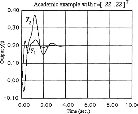
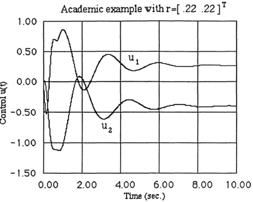
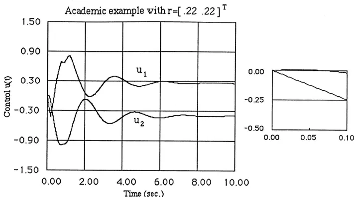
Figures 4.3 and 4.4 show the output and control responses for the linear system. The controls violate the +1 limits and the rate of the controls exceed the +2.5 limits. The linear response is assumed to be the desired one.

Figures 4.5 and 4.6 show the output and control responses of the system with magnitude saturation. One can see that the output response has significantly deteriorated even for a small amount of saturation (= 1.1).

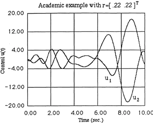
Figures 4.7 and 4.8 show the output and control response of the system with both magnitude and rate saturation. The response of the system has now completely deteriorated in both the controls and the outputs.

Academic example vithr=[ .22 .22]

0.00

-0.10

-0.20

Academic example with r=[ .22 .22

1.50

0.90

0.30

-0.30

-1.50

0.00

2.00

4.00

6.00

8.00

10.00

Figure 4.4: Control of the linear system with reference (r = [ .22 .2 2]T). Insert: Blowup with

O<t<.l sec

Academic example

with

0.40

0.30

' 0.20

o 0.10

-0.10

0.00

2.00

4.00

6.00

8.00

10.00

Figure 4.5: Output of the system with control magnitude saturation, without control rate saturation and with reference (r = [ .22 .2 2]T)

Academic example vith r=[ .22 .22 ]

0.50

-0.50

-1.00

-1.50

0.00

2.00

4.00

6.00

8.00

10.00

Figure 4.6: Control of the system with control magnitude saturation,without control rate saturation and with reference (r = [ .22 .2 2]T)

Academic example vithr=[ .22 .22 ]T

2.00

0.80

-0.40

o -1.60

-2.80

-4.00

0.00

2.00

4.00

6.00

8.00

10.00

Academic example vith r=[ .22 .22

-12.00

Figure 4.8: Control in the system with control magnitude and rate saturation, (r = [ .22 .2 2]T)

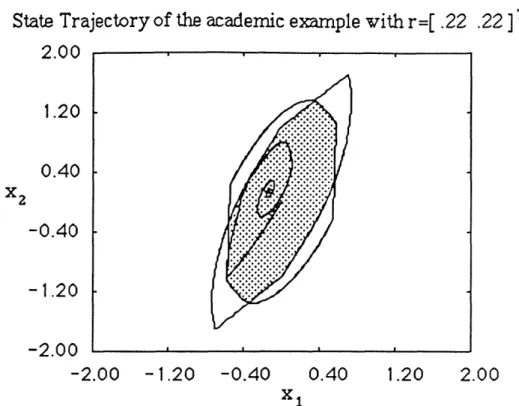
Figure 4.9 show the state trajectory of the system with magnitude and rate saturation and the EG operator. Note that the state trajectory of the compensator does remain in SA,c for all t and

so neither magnitude nor rate saturation will occur.

Figures 4.10 and 4.11 show the output and control response of the system with the EG operator. Note that the output direction is similar to the linear response and that the controls remain within the limits of the magnitude and rate saturation.

Figure 4.12 show the X(t) required for this simulation. One can see that the X(t) starts at a value less than 1 since the controls at the beginning would exceed the rate saturation limit then

gradually X(t) increases to 1, then the states of the compensator reach the boundary of the RA,C set and X(t) is decreased. Note that ,(t) is also decreased drastically again at =.6 sec, because the states of the compensator reach the boundary of the BA,C set.

State Trajectory of the academic example vith r=[ .22 .22 ]

2.00

1.20

0.40

x

-0.40

- 1.20

-2.00

-2.00

-1.20

-0.40

0.40

1.20

2.00

Figure 4.9: State trajectory of the system with control magnitude/rate saturation and the EG, (r = [ .22 .2 2]T)

Academic example vith r=[ .22 .22 ]

0.30

0.20

'

-0.10

-0.20

0.00

2.00

4.00

6.00

8.00

10.00

Academic example vithr=[ .22 .22

1.50

0.90

0.30

-1.50

0.00

2.00

4.00

6.00

8.00

10.00

Figure 4.11 _{l: Controls in the system with magnitude and rate saturation and the EG,} (r = [.22 .2 2]T). Insert: Blowup of 0 < t < .1 sec

a (t) for the academic example vith r=[ .22 .22 ]T 1.10 0.88 _1.20 0.66 0.80

x

Figure 4.12: X(t) of the system with magnitude/rate saturation and the EG, (r = [.22 .2 2]T).

5.0 CONCLUSION

In the presence of saturations the stability and performance of a linear control system can suffer. Saturations can also affect the performance of the control system by introducing reset

windups and by changing the direction of the control signal. Large overshoots and oscillatory outputs are the consequence.

A systematic methodology was introduced for the design of control systems with multiple saturations in control magnitude and rate. The idea was to introduce a supervisor loop; and when the references and/or disturbances are "small" enough so as not to cause saturations, the system operates linearly as designed. When the signals are large enough to cause saturations, then the control law is modified in such a way to preserve, to the extent possible, the behavior of the linear control design.

It has been shown that the operator EG can be used to design control systems when the controls saturate in magnitude and rate. The main benefits of the methodology are that it leads to controllers with the following properties:

(a) _{The signals that the modified compensator produces never cause saturation.} (b) _{Possible integrators or slow dynamics in the compensator never windup.} (c) _{The closed loop system has inherent stability properties.}

(d) The on-line computation required to implement the control system is feasible. An academic example was used to illustrate the methodlogy and its benefits.

REFERENCES

[1] M. Athans, P.L. Falb, Optimal Control, New York, McGraw-Hill, 1966.

[2] C.A. Harvey, " On Feedback Systems Possessing Integrity With Respect to Actuators Outages", Proceedings of the ONR/MIT Workshop on Resent Developments in the Robustness Theory of Multivariable Systems, LIDS-R-954, M.I.T., Cambridge, MA, April 25-27, 1979.

[3] A. Weinreb and A.E. Bryson," Optimal Control of Systems with Hard Control

Bounds" IEEE Transactions on Automatic Control, Vol. AC-30, No. 11, November 1985, pp. 1135-1138.

[4] P. Gutman and P. Hagander, " A New Design of Constrained Controllers for Linear Systems", IEEE Transactions on Automatic Control, Vol. AC-30, No. 1, January 1985, pp. 22-33.

[5] A. H. Glattfelder and W. Scaufelberger," Stability Analysis Of Single Loop Control Systems with Saturation and Antireset-Windup Circuits", IEEE Transactions on Automatic Control, Vol. AC-28, No. 12, December 1983, pp. 1074-1081.

[6] R. Hanus, " A New I'echnique for Preventing Windup Nuisances", Proc. IFIP Conf. on Auto. for Safety isLT hipping and Offshore Petrol. Operations, 1980, pp. 221-224.

[7] P. Kapasouris, M. Athans, G. Stein, Design of Feedback Control Systems for Stable Plants with Saturating Actuators, Proceedings of the 27th IEEE Conference on Decision and Control,Austin, TX, December 1988, pp. 469-479.

[8] P. Kapasouris, M. Athans, G. Stein, Design of Feedback Control Systems for

Unstable Plants with Saturating Actuators, Proceedings of the 1989 Nonlinear Control System Design, IFAC, Capri, Italy, June 1989.

[9] P. Kapasouris, Design for Performance Enhancement in Feedback Control Systems with Multiple Saturating Nonlinearities, Ph.D. Thesis, Department of Electrical Engineering, M.I.T., Cambridge, MA, February 1988.