The effect of magnetic pinch pressure on boron nitride, cadmium sulfide, graphite, silica glass, and some other materials.

THE EFFECT OF MAGNETIC PINCH PRESSURE ON

BORON NITRIDE, CADMIUM SULFIDE, GRAPHITE, SILICA GLASS, AND SOME OTHER MATERIALS

by

STEPHAN JAY BLESS

S.B., Massachusetts Institute of Technology

(1965)

S. M., Massachusetts Institute of Technology (1968)

SUBMITTED IN PARTIAL FULFILLMENT OF THE REQUIREMENTS FOR THE

DEGREE OF DOCTOR OF SCIENCE at the MASSACHUSETTS INSTITUTE OF TECHNOLOGY June, 1970

Signature of

De n f Earth and Planeta ciences,/nlay 21, 1970 Certified by ... I / _{Thesis Supervisor}

Accepted by

WiTFpORAWN

ES

ABSTRACT

We have developed a new method of high pressure production which

uses a capacitor-discharge driven magnetic pinch. The pinch is capable of

producing pressures greater than 500 kilobars, and is superior in several

respects to other current high pressure techniques. Observed pinch effects

include: production of the zincblende phase of boron nitride, production of

hexagonal diamond from graphite, decomposition of mullite to alumina plus

amorphous silica, and irreversible densification of powdered and solid silica

glass. The resistance discontinuity sometimes seen in cadmium sulfide at

28 kilobars and the decomposition of albite to jadeite plus quartz did not

occur. Some discrepancies between pinch results and those of conventional

techniques can be explained by the heating which follows pinch pressure

max-imum. This latter condition can probably be eliminated by modification of

the pinch apparatus.

TABLE OF CONTENTS

Abstract 2

List of Symbols 5

Photographs 7

1. INTRODUCTION

1.1 Major Problems in High Pressure Geophysics

1.11 Phase transformations in the mantle 11 1.12 High pressure melting of geophysical materials 13 1.13 Electrical properties of the core 15 1.2 Role of the Magnetic Pinch

1.21 Limitations of static pressure devices 16 1.22 Limitations of shock wave techniques 16

1.23 The magnetic pinch device 18

1.24 Previous pinch research 18

1.25 Advantages of the magnetic pinch 19

1.3 Production of Megagauss Magnetic Fields

1.31 Exploding wires and plasma confinement 20 1.32 Production of megagauss fields with chemical explosives

20

1.33 Production of megagauss magnetic fields by capacitor discharge

22 II. APPARATUS

2.1 Discharge Circuit

2.11 The capacitor bank 24

2.12 Sample design 27

2.13 Computation of maximum current 29

2.14 Calculation of circuit inductance 31

2.15 Measurement of the current 34

2.2 Effects of the Pinch

2.21 Production of high pressure 39

III. EXPERIMENTAL INVESTIGATIONS

3.1 Quartz

3.11 High pressure data on quartz

3.12 Pinch experiments on fused quartz

3.13 Conclusion from pinch data

3.2 Boron Nitride

3.21 High pressure phases of boron nitride

3.22 BN experiments

3.3 Cadmium Sulfide

3.31 Cadmium sulfide high pressure polymorphs

3.32 Pinch experiments with cadmium sulfide

3.33 Interpretation of pinch experiments

3.34 Discussion of results

3.4 Carbon

3.41 High pressure polymorphs of carbon

3.42 Pinch experiments on graphite

3.43 Observations on pinch experiments

3.5 Albite

3.51 High pressure instability of albite

3.52 Pinch experiments with albite

3.6 Mullite

IV. CONCLUSIONS

4.1 P-T History of samples

4.2 Recapitulation

4.3 Suggestions for Future Work

V. ACKNOWLEDGEMENTS

VI. APPENDICES

Al. Complete Data for all Shots

A3. Experiments with Iron

A4. Variation of Pressure within the Spool

A5. Details of Refractive Index Measurements

A6. Stress and Strain within Sample

VII. REFERENCES 94 97 99 102 103 108 111 113 118 125 129

LIST OF SYMBOLS

A

Area, constant parameter

B

Magnetic flux density, constant parameter

C

Capacitance, heat capacity, constant parameter

C

Capacitance of one capacitor

=

15 pf

D

Constant parameter

d

diameter of spools, spacing of crystal planes in Angstroms

diameter of spools in mm

6

phase angle

E

voltage, Young's modulus

emf

e

permittivity

I

current, X-ray intensity

K

bluk modulus, thermal conductivity

L

inductance

L

inductance of one capacitor and spark gap

L

inductance of transmission line and sample

L

inductance of aluminum plates

L

inductance of sample

A

permeability

-7

14

permeability of free space

=

4 x 10

h/m

0

N

number of capacitors

n

index of refraction

P

pressure, power

P

pinch pressure

Q

charge, thermal energy

R

resistance,

gas

constant

R

spool resistance

/0p

resistivity

p

mass density

r

radiu s

a

stress, conductivity

s

specific heat, skin depth

T

period, temperature

T

period in Psec

U

energy

V

voltage

V

voltage measured in kV

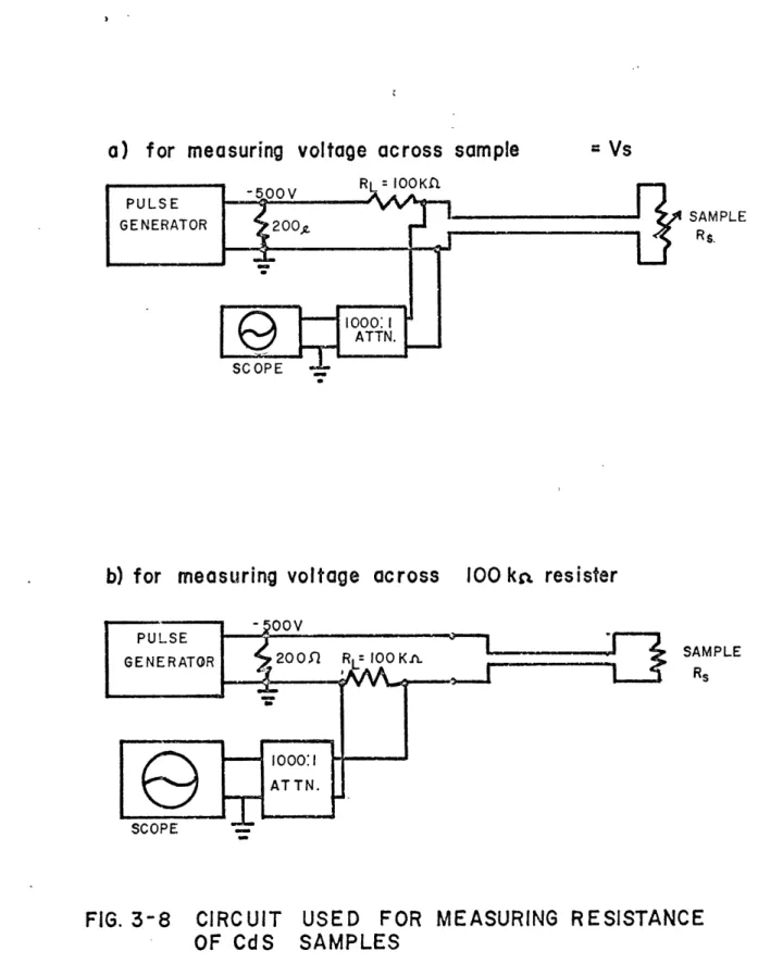
V

voltage across sample

VL

voltage across series resistor

Z

impedance

Photo 1

Capacitor bank and transmission line.

Photo 2

Sample assembly parts.

(Numbered items discussed in text.)

Photo 3

Typical oscillograph.

(For shot S6: N = 4, V = 14. . kV) Sweep is 2 .,scc/div.

Upper trace: Rogow\ski coil outpu, 200() \ Lower trace: InteCgrator Output. 40 V di\

Photo 4

-Cross section of fused quartz rod, after pinch and after copper spool has been dissolved (shot T2) Diameter of quartz rod is

.0303 inch. (Initial diameter was .031 + .0005 inch.)

Photo 5

-Cross section of CdS sample after

pinch (shot E 24) _{". . .}

Photo 7

-Comparison of new spool with one of "little" damage (shot GQ2)

Photo 8

-Comparison of new spool with one of "great" damage (shot A2)

Photo

9-Sample chamber after shot in which spool was "destroyed" (shot D2)

I. INTRODUCTION

1.1

Major Problems in High Pressure Geophysics

Much progress has been made in high pressure geophysics in the

last decade. High pressure polymorphs of many minerals have been

dis-covered, and the pressure dependence of elastic and thermodynamic

parameters have been investigated. The purpose of this section is to

point out several important questions which cannot be answered by current

high pressure technology. These are problems concerning the structure

and composition of the earth below about 500 kilometers. These are also

the problems which we hope the development of magnetic pinch techniques

will resolve.

11 1.11 Phase transitions in the mantle

Birch (1952) was the first to apply modern elastic theory and high pressure experimental results to the study of the mantle. Using the appro-priate seismic velocity-depth relationship available at that time, he deter-mined that the velocity increase between 200 and 900 kilometers was not consistent with a self-gravitating homogeneous medium; below that, to the core, it was. He suggested that the velocity increase was due to the re-duction of normal magnesium-silicates to denser oxide structures, a pre-diction which has been verified by subsequent experimental results.

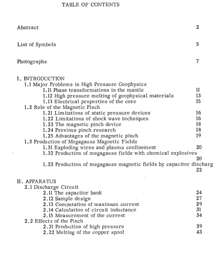
I S Fig. 1-1

I Distribution of seismic

' P wave velocities in

the outer 1200

kilo-o - I meters of the mantle.

I (after Archambeau et.

I a I I Z I UPPE I I I I 0 200 f00 600 g oo /00 20oo i0o DEPTH KM

Figure 1-1 is an example of modern determinations of the seismic velocity-depth function. It will be seen that in addition to the general trends known to Birch, several clear discontinuities exist . At lower depths, Toksoz et. al. (1967) have recently discovered additional sharp increases at 700, 1200, and 1400 kilometers. zMcDonald' s (1957)

12

derivation of the electrical conductivity of the mantle also implies a dis-continuity between 500 and 700 kilometers.

The lower mantle is believed to be largely composed of magnesium, silicon, and oxygen (see, for example, Ringwood, 1966). The common minerals composed of these elements are Mg2SiO4 (fosterite), MgSiO₃

(enstatite), MgO (periclase), and SiO2 (quartz). It is very important to

know how well the seismic and conductivity measurements can be explained by the high pressure properties of these minerals and their polymorphs.

The pressures occurring in the middle and lower mantle cannot be duplicated in present static apparatus, and shock wave techniques cannot be used because much overdriving is required to produce high pressure silicate polymorphs (see, for example, McQueen et. al., 1967). However, many high pressure properties of silicates can be inferred from study of germanate isomorphs (see, for example, Ringwood & Seabrook, 1962). Analogous high pressure phases form at power pressures in germanates because of the larger size of the germanium ion. Ringwood (1968) and others predict the following high pressure modifications of magnesium-silicates: Mg2SiO4 (spinel structure), MgSiO3 (ilmenite structure), MgO

(CsCl structure), MgSiO_{3 (perovskite structure), Mg}

2SiO4 (Sr 2PbO4

structure), and Mg3(MgSi)Si30 12 (garnet structure). However, the P-T

stability fields of these polymorphs have not been directly studied. Nor (except for shock wave analyses) have there been measurements of their elastic or electrical properties. Moreover, the entire concept of using germanate isomorphs to predict silicate phase transitions is made suspect

by the recent discovery of a unique Mg2SiO4 structure which does not

1.12 High pressure melting of geophysical materials

The study of melting phenomena is one of the few means available for estimating temperature in the interior of the earth. Let us designate T and T. as the temperature at the upper and lower boundaries of the

o t

outer core (where the pressure is 1.4 and 3.2 megabars, respectively). Determination of the pressure dependence of melting for lower mantle consituents (such as MgO, SiO2 or _{A1203) can place an upper limit on To.} Determination of the fusion curves for probable core constituents (iron-silicon alloys) can place a lower limit on T and an upper limit on T..

(If the fusion curve has a maximum, T. may even be precisely determined.)

The practical obstacles to this program are three-fold: (1) Fusion curves can only be empircally determined to a few hundred kilobars. (2) The methods used for extrapolation of fusion curves to higher pressures are of dubious validity. and (3) The actual composition of the earth is unkown.

Several studies of the melting of possible core materials have been carried out (for example, Sterrett et. al., 1965, Boyd & England, 1963, Strong, 1962), but no data has been taken above 200 kilobars. Ideally, melting could be studied at much higher pressures by using shock waves, but in practice, the onset of fusion is very difficult to detect because it has almost no effect on the PV hugoniot (see McQueen et. al., 1967, fig. 17a). Very seldom can the discontinuity in the u vrs. u hugoniot caused by

s p

There are several melting relations which may be used to extrapolate

low pressure data to core conditions. Historically, the most important

is the Simon equation, developed to describe the melting of helium (Simon,

1929):

P-P

a - 1 (1.1)

in which P and T are reference fusion curve coordinates, and a and c

O O

are adjustable constants. Kennedy (1970) has shown that this equation can

only be expected to hold for solids which are bound by Van-der-Waals

over estimates the melting temperature at high pressure.

The Lindemann melting law (see Roberts & Miller, 1951, for a simple

derivation) is derived from the assumption that a solid melts when the

amplitude of the thermal oscillations becomes a certain fraction of the

interatomic spacing. Gilvarry (1955) has expressed the Lindemann law

in the form

RT

=

? K V

(1.2)

m

mm

where Tm , K , and V

are evaluated at the melting point, R is the gas

mm

m

constant, and P is a constant which depends on Poisson's ratio and the

nearest neighbor distance at melting. Gilvarry also showed that for ym

(the Gruneisen contant of the solid at fusion) greater than 1/3 (which is

always true at high temperature) Tm will be a monotonic-increasing

function of pressure. Although the Gilvarry formulation of the Lindemann

law works rather well for many metals (KInopoff, 1970), it can n-ever predict

the fusion curve maxima which have been discovered in several others

(Newton, 1966, fig. 21).

Krout and Kennedy (1966) and Kennedy (1970) have observed that

T =T (1 + C )

m 0 V

for most metals and silicates. (Here \V/V is the relative compression

at fusion, and C is an adjustable constant.) Gilvarry (1966) has shown that this relationship is an approximation to (1.2) which ignores terms of the order (V - V )2 . _{Therefore, it should not be used for extensive extrapolations.}

In summary, neither equation (1.1) nor equation (1.2) can be used to predict melting deep within the earth without some input of data obtained under extreme pressure. Nor can they describe melting of solid solutions,

in which eutectic effects can dramatically lower melting temperatures (Newton, 1966).

1.13 Electrical properties of the core

Another area of importance is the study of the electrical properties of materials likely to compose the earth's fluid core. The variables re-quired for hydrodynamic analysis of motions in the core are density, conductivity, permeability, and viscosity. The dynamic processes possible in the core are largely determined by the Value of the magnetic Reynolds number

(thickness) x orp

and certain dimensionless scaling parameters (see, for example, Hide, 1966). Yet, at the present time, no relevant experimental data for these parameters has been obtained.

1.2 Role of the Magnetic Pinch

1.21 Limitations of static pressure deirices

Truly hydrostatic pressures (in which the pressure transmitting

medium is a fluid) are only possible well below 50 kilobars. All solid

media devices suffer from stress anisotropy, which can be very large.

Pressure can be calibrated by means of known phase transitions or

com-pressibilities to an accuracy of a few percent; temperature under pressure

can be measured with thermocouples, but the errors are not known

(see, for example, Strong, 1962).

Most existing equipment is designed

to operate below 100 kilobars. There are a few laboratories where

uniaxial pressures to 200 kilobars and temperatures to 1000'C can

be produced (Ringwood & Major, 1966, Akimoto & Ida, 1966 , 3undy, 1965),

but volume cannot be measured as a function of pressure, and structure

determinations must be done with quenched materials. Those laboratories

which can produce pressures of 200 kilobars and obtain X-ray patterns

under pressure must operate near room temperature. (Bassett, 1967,

Drickamer, 1966).

1.22 Limitations of shock wave techniques

Production of intense shock waves in solids can result in transient

pressures as high as five megabars (Doran & Linde, 1966).

However, the

duration of the pressure pulse is a small fraction of a microsecond, and

the strain is one-dimensional. (See Rice et. al., 1958, for an introductory

discussion of shock wave production and analysis.) Shock wave experiments

require rather expensive facilities, so only a few authors have been active

in this field. Analyses of shock data have yielded high pressure equation

of state, electrical, and optical parameters; most of the geophysical

re-sults are discussed by Ahrens et. al.(1969).

However, there are serious

ambiguities concerning the application of shock wave data to the study of

the earth. The difficulties in interpretation fall into three catagories:

(1) The elementary fluid theory and jump conditions used to derive hugoniots

may be wrong (Fowles et. al., 1970). (2) All of the various algorithms for

reducing shock hugoniots to isothermal or adiabatic data (for example,

Ahrens et. al., 1970, Munson & Barker, 1966, McQueen & Marsh, 1967,

Duvall & Fowles, 1963) require assumptions about the pressure dependence

of the Gruneisen constant, hydrostatic stress, and constitutive relations

which are not well substantiated. (3) Phase changes which require more

than simple displacement of atoms may not have time to occur (such as

olivine to spinel), or may not occur at the equilibrium pressure (such as

graphite to diamond).

Fig. 1-2

Magnetic Pinch geometry

Q

1.23 The magnetic pinch device

The geometry of the magnetic pinch effect is illustrated in figure 1-2.

A large current is established in a straight conductor. A magnetic field

B = o

2 rTr

is set up around the conductor. The field exerts a force

F = q vXB

on the current carrying electrons. Thus the electrons experience a

pressure equal to the magnetic pressure

B

P

-Since the electrons are bound to the atoms, the pressure is felt by

the solid material. In practice, the current is supplied by discharge of a

high energy low inductance capacitor bank. The linear conductor is a

hol-low cylinder, and the material to be studied is placed inside.

1.24 Previous pinch research

Only Bitter et. al. (1967) and Bless (1968, 1969) have reported

appli-cation of a magnetic pinch to high pressure research. They found that:

a) Magnetic pinch pressure could produce the ,g,- - phase transition

in iron, which at room temperature occurs at 130 kilobars.

b) The ability of solid rods to survive destruction by the pinch current

was enhanced by radial reinforcement. This suggested that the principle

mechanism of failure (aside from simple melting) was development of

c) The energy which is deposited in the sample being pinched was al-ways much less than the energy stored in the capacitor bank.

d) High pressure polymorphs of quartz could not be recovered from pinch experiments on fused quartz.

1.25 Advantages of the magnetic pinch

At its present stage of development, the pinch offers little advantage over conventional high pressure techniques. However, looking foward to the solution of what appear to be straightfoward technical problems, we can forcast that the pinch will:

a) Allow measurements of elastic and electrical properties at pressures of one megabar.

b) Compress materials adiabatically, with well defined P-T con-ditions.

c) Allow more accurate pressure determination than shock waves, since the pressure is a simple function of the current.

1.3 Production of Megagauss Magnetic Fields

1.31 Exploding wires and plasma confinement

The technology which permits construction of ultra-low inductance

high energy capacitors has only been in existence for about ten years (see,

for example, Frungel, 1965).

Two traditional research areas where

cap-acitor discharge techniques have found application are plasma pinch effects

and electrically exploded wires. Neither of these efforts are directed

toward producing kilobar pressures in solids. Rather, plasma confinement

requires pressures of a few hundred bars containling volumes of many

cubic centimeters. Exploding wire studies emphasize maximum energy

input (primarily for explosive detonation).

Bless (1968) reviews the

research results in these two fields and lists an extensive bibliography.

1.32 Production of megagauss magnetic fields by chemical explosives

Fig. 1-3

The relation between

magnetic field and

pressure.

(After Bitter, 1965)

0-10

MAGNETIC FIELD (GAUSS)

FUTURE IMPLOSION TECHNIQUES (MICROSECONDS") PRESENT RE IMPLOSION TECHNICUES (MICROSECONDS)

SMALL COILS ACTIVATED BY CAPACITOR DISCHARGES (MILLISECONDS) AIR-CORE SOLENOIDS (CONTINUOUS) IRON-CORE ELECTROMAGNETS (CONTINUOUS) I

Francis Bitter (1965, 1967) was the first to point out the possible

application of ultra-high magnetic fields to high pressure research.

Figure 1-3 illustrates the relationship between magnetic flux density

and pressure. Although considerable progress has been made in the

laboratory production of megagauss magnetic fields, with the exception

of the author's work, no practical application has been attempted.

How-ever, many of the technical problems encountered in high magnetic field

production carry over to the pinch work discussed in this paper.

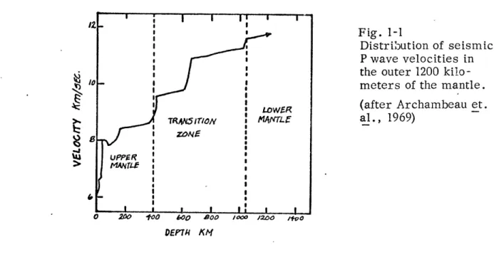
Figure 1-4 Typical geometry for flux compression by explosives.

(After Bitter, 1965)

Figure 1-4 shows the geometry for explosive flux compression. A

magnetic field of typically 100 KG is established inside a seamless cylinder

(called a liner) with a typical radius of 5 cm. This is accomplished by

capacitor discharge, typically about 100 kilojoules with a time constant of

10-

seconds. The field diffuses into the liner in the characteristic time

T

=

M rd/2p

(Latal, 1966)

where r

=

liner radius, d

=

liner thickness,

p

= liner resistivity, and

o =

4 17x 10

h/m. The liner is compressed by explosives, trapping the

"seed" field inside. The maximum field reported by this technique is 10 MG

(Besangon, 1967).

Keeler (1970) is presently adapting this type of apparatus

to high pressure research.

The maximum compression occurs when the magnetic pressure in

the liner equals the pressure of the chemical explosive. The maximum

attainable field will depend on the properties of the liner material, viz.

the increase in liner resistivity and its equation of state. Eventually,

joule heating of the': liner will convert it to a plasma; then the resistivity

decreases as the 2/3 power of temperature. Unfortunately, the differential

equations linking these phenemena have not been solved for the general

case (see, for example, Herlach, 1968).

Lewin and Smith (1964) obtained

an approximate solution, which applied to Fowler's (1960) experiment

pre-dicts that the final pressure coefficient of resistivity of the liner (copper)

was not greater than 1/200th its usual value. The final P-T conditions were

approximately 2x10

'K and 8 megabars.

1.33 Production of megagauss magnetic fields by capacitor discharge

Two methods of producing megagauss magnetic fields by capacitor

discharge have been tried. The first, developed by Cnare (1966), utilized

electromagnetic compression of a cylindrical aluminum foil. The foil was

Sufficient flux leaked through the aluminum foil before implosion that a

peak field of over 2 MG was produced within it. The theory of the "Cnare

Effect" has been developed by Latal (1967). Further experimental work has

been done by Guillot (1968).

The other means of producing high magnetic fields by capacitor

discharge is to use a single turn coil. Shearer (1969) has been the principle

investigator of this method. The maximum field he has obtained is about

3 MG. X-ray photographs of the massive copper coil during the discharge

showed a compression of about 10% (in linear dimension), suggesting a

shock pressure of about 200 kilobars. He calculated the interaction of the

field with the metal wall and predicted that a shock type discontinuity would

appear after the pressure wave had travelled about 4mm into the copper.

Shearer also observed that under some conditions the surface of the wall

moved into the high field region because of the rapid heating due to skin

effect.

11. APPARATUS

2.1 Discharge Circuit

2.11 The capacitor bank

The large currents required to produce high pinch pressure were obtained by discharging a high energy low-inductance capacitor bank. The basic arrangement of the capacitors was similar to that described by Bless (1968). There were eight Tobe Deutschmann model ESC-248A capacitors. Each was 15 pf, 20 kV, 3000 joules, making a total of 120 14 f and 24 kilo-joules. They were arranged around an octagonal transmission line, designed for low inductance. Photo I shows this equipment. Any combination of the capacitors could be fired at one time; however, the lowest voltage at which simultaneity was obtained was 14 kV.

Figure 2-1 is a sketch of the capacitor and trigger circuits. The capacitor power supply was located outside of the instrument cage, in order to avoid ground loops. The charging voltage was pre-set, and the operator enclosed himself in the shielded instrument cage (which was also armoured with plywood). The highest charging voltage that could be used was 40 kV, otherwise there was danger of arcing across switch A. The "outside

meter" could be read froni inside the cage. When the bank voltage reached the desired value, the oscilloscopes were triggered. A gate pulse from one of the scopes was used to initiate the pulse sequence that resulted in firing of the spark gaps. Residual charge on the capacitors could be drained by activating a 10 megaohm dump relay in the power supply. If the sample was destroyed, it was necessary to close switch B for this operation. When not

DOUBLE SGREEN

INSTRUM4.EN

T

ROOM

OUTSIDE

1:1

PULSE

TRANS.

OSC LLOSCOPE.

LOWER

TRANSMISION

PLATE

FIG.2*-

CIRCUIT DIAGRAtA

, SHOWING

ONE

OF EIGHT CAPACITORS.

SWITCHES ARE IN CHARGING

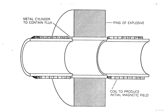
FIG. 2-2

r

o2

zzzI"lzz

4 15

5

6

18

4

EIIIZIZ

SAMPLE

ASSEMBLY

---,.0

I-27

in use, switch A was connected to a 1 megaohm bleed resistor. As an extra precaution, each capacitor was checked for zero charge with- a grounding pole

after every shot. Power supply ground (G1 in figure 2-1) was a cold water pipe,

while instrument ground (G2 in figure 2-1) was an electrical conduit. There was never a direct connection between the two.

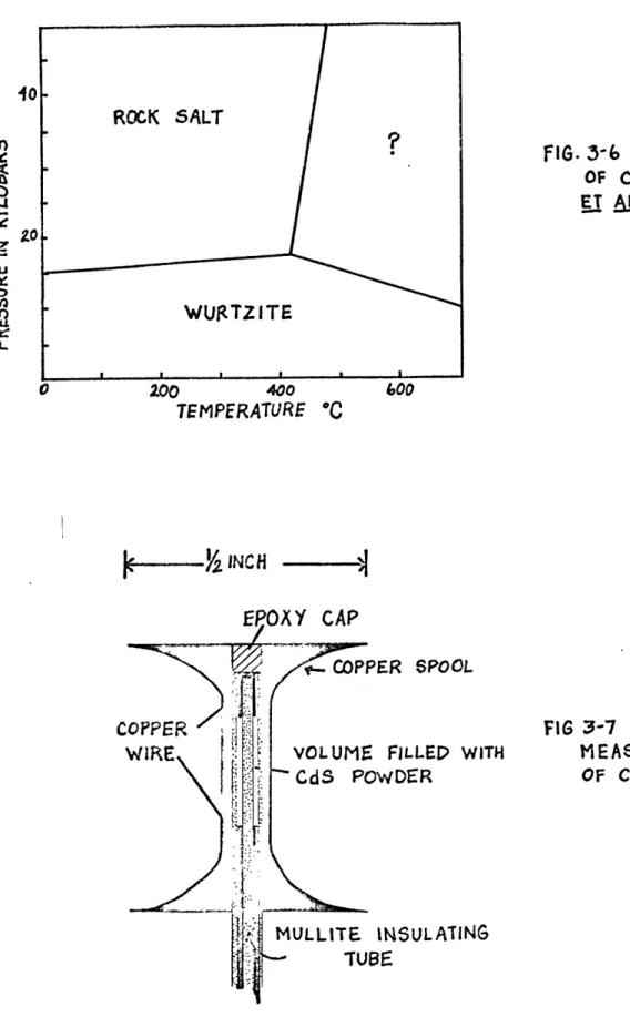
2.12 Sample design

The current which produced the magnetic pinch was carried by cop-per spools, like the one shown in photo 2. The shaft diameter was almost al-ways .115 inches (2.92 mm); the length was .545 inches. The spools had a .065 inch (1.65 mm) diameter hole along their axes. Usually, the centers of the spools were fitted with insulating tubes which contained the materials to be studied. In this paper, the word "sample" refers to the contents of the copper spools.

The spools were connected across the two octagonal transmission plates by the sample assembly, shown in photo 2 and figure 2-2. The impor-tant parts are numbered:

1) Upper phenolic clamp block.

2) Steel impact block to absorb recoil of spools.

3) .020 inch thick copper discs, which made connection to the spool: 4) 3/8 inch thick center of aluminum transmission plates.

5) .010 inch copper connecting sheets. 6) Six .010 inch mylar insulating sheets.

7) Copper spool which contains sample. The spool was often encased

in epoxy.

28

9) Steel guard ring, to contain material thrown off spool; O-ring

seal-spring on bottom. The guard ring was often shimmed on the bottom to insure a good blast seal on top.

10) Phenolic insulating ring, with O-ring seal on top.

11) Lower clamp block, with 1/8 inch hole which could be used to

hook up experiments inside the spool (for which purpose a hole was drilled in the lower impact block).

12) upper anvil, which threaded into top of aluminum plate structure

(see photo 1).

13) lower anvil.

A relatively large amount of time was required to keep the sample

assembly in good condition. Generally, shots producing less than about 50 kilo-bars caused little damage. During shots of 50 to 200 kilobars, much of the copper spool melted, the epoxy coating on the spool was partially pulverized, and the blast and soot degraded the mylar insulating sheets. After approxi-mately every other such shot, the lower-most mylar sheet had to be replaced, in order to be certain that the insulating ring O-ring made a good seal. After about five shots, all the mylar sheets and copper connecting sheets had to be replaced. Shots producing over 200 kilobars often did great damage, for unless the tolerances were extremely tight, hot gases and ejected material tore the top copper sheet and cracked the mylar. Pressure waves from these shots

often expanded the guard ring by more than .010 inch, and excavated holes up to 1/4 inch deep in the impact blocks. Sometimes, the clamp blocks even

29

At the present time, one person can replace the insulating sheets in about 90 minutes. This is an improvement over the time required at our last

report (Bless, 1968), when half a day was required by two people. The reduction

resulted from several modifications in the plate design which simplified parting

the center sections of the aluminum plates.

The average time required to set up, perform, and repair after a

100 kilobar shot was about four hours. Including manufacturing charges for

samples and spare parts (and excluding the value of the experimenter's time),

the cost per 100 kilobar shot was about $10. The initial cost of the capacitor bank and power supply was about $6000.

2.13 Computation of maximum current

The charge stored in the capacitors is

Q =

N can be varied from 1 to 8, C = 15 f, and V can be varied from 14 to 20 kV.

(N, V, C , and Q are defined in the list of symbols.) The maximum value of Q

is 2.4 coulombs. The maximum energy, given by

U NC V2 (2.2)

2

o

is 24 kilojoules, or 5760 calories (gram).

The current which flows through the copper spools is

I(t)

=

dQ/dt.

For a decaying oscillatory discharge (see, for example, Harnwell, 1949, p. 458)

Qo

-Rt/2L

Q

=

-

e

sinh

R2/4L2

1/LC t .

R2C

For the limit R

-+

0, equation (2.4) becomes

Q

= Qo cos wt

w. = 1/ LC _and

_Q

In our experiment, R is a function of time and is not zero.

less stringent condition R

Qo

4L

< 4L/C, equation (2.4) becomes

-Rt/

L

1

R

sin(C

4 L

6

arctan

It is difficult to evaluate the.term (4L/R2C) because the resistance

of the copper spool and spark gaps changes as the current flows. A rough

es-timate can be made by examining a typical current record. For example,

in figure 2-7b, with N

=

2 and V

=

17 kV, the amplitude decay gives

2L

R

16 psec.

(2.9)

From the period:

T - 2rr,LC

VLC

_{- .717 x 10}

.717

10-6

4.5

10-6

4.5 x10

sec

sec

.

Putting equations (2.9) and (2.11) together gives

2

2

-

2

)

where

(2.6)

S4L

R2C

(2.8)

31

Therefore, for purposes of calculating discharge current we may use the ap-proximation

I = -'

Qo

The maximum of I occurs at t = Y , and is

I(max)

Writing T _

2_rr

'ni,~7

Qo4LC . (2.13)

4sec, V = V kV, and combining 2.1 with 2.13 gives (max) 2N C2 V

T = 94.2 x 103

NV

T

(2.14)

2.14 Calculation of circuit inductance

Fig. 2-3

Circuit for computation of effective inductance

N units

Figure 2-3 represents the circuit which must be analysed to com-pute the effective inductance. If Q is the charge on a capacitor C , Kirchoff's rule for this circuit is:

C

L

2Q Lf

i Q

Q

L d2

-

N

Q

Qo

L = the inductance of a capacitor and spark gap

LL = the inductance of the transmission lines and sample

In Bless (1968) it is calculated that

(2.17) L = 11.7 nanohenries .

0

Since

L = /I , B = I/2nr, and _= B- dS,

we can write L, as the sum of two terms, LI = L +L ,

p s

where L is the

P contribution to Lp from the flux contained between the trans-mission lines, and L the the inductance from the flux contained in the sample

a

assembly. In Bless (1968) it is also calculated that L = .747 nanohenries = 0 = 0 where = / L O (2.15) (2.16) (2.18)

Fig. 2-4

Geometry for calculation

of contribution to the inductance

of the copper spools. X

Figure 2-4 is a simplified drawing of the interior of the sample

assembly.

=

tr Idy

dx

S

x

(2.19)

This integral was evaluated by dividing the curved portions of r(x) into three

steps; its value was 6.54 I.

L = 6.54 nanohenries,

s

(2.20)

for a 2.92mm diameter spool.

From equations 2.6, 2.16, 2.17, 2.18, and 2.20, the total inductance

for a discharge of N capacitors is

L

11.7 + N(7.29)

nanohenries .

For example,

L = 67 nanohenries when N = 8.

The theoretical disc harge periods, calculated from T = 2-Co(Lo + NL)

.00

are listed below:

(2.21)

34

N

1

T

3.4 Asec

N

6

T

5.72 psec

N =8

T

5.85 psec.

Appendix Al gives all the observed values of T. The agreement is fair at low voltages and good at high voltages. The dependence of T on vol-tage arises because the spark gaps have less resistance and inductance at high voltages.

According to this analysis, the maximum current which can be produced in a 2.92 mm diameter spool is given by equation (2.14) with T= 5.85, N = 8, and V = 20; e.g.

I( m a x ) = 8.44 x 106 amperes. (2.23)

2.15 Measurement of the current

In order to measure the pinch current, a Rogowski coil was made by lacing flat copper ribbon through one of the mylar insulating sheets. Figure 2-5 shows the.coil geometry. The ribbon was .005 inch by 1/16 inch. The cross

-6 2

section of the coil was 1 1/2 inch by .010 inch, or 9.67 x 10 m . There were 60 turns, and the mean distance from the center of the copper spools was 14 1/2 inches (.362 m). It was wound back through itself to reduce sensitivity to azimuthal current inhomogeneities.

Fig. 2-5

_E7'

Rogowski coil geometry

The voltage induced in the Rogowski coil is readily calculated from Maxwell's relation:

-

at

-t

Here,

dB

S= nAd

where F is the total emf induced in the coil, n is the number of turns, and

A is the toroidal cross sectional area. Since

po I

B P

2Tr

o A nNw'

2rrr

Equation (2.24) is evalued for V = VkV,

PO-u

2

V sin ut

max)

T

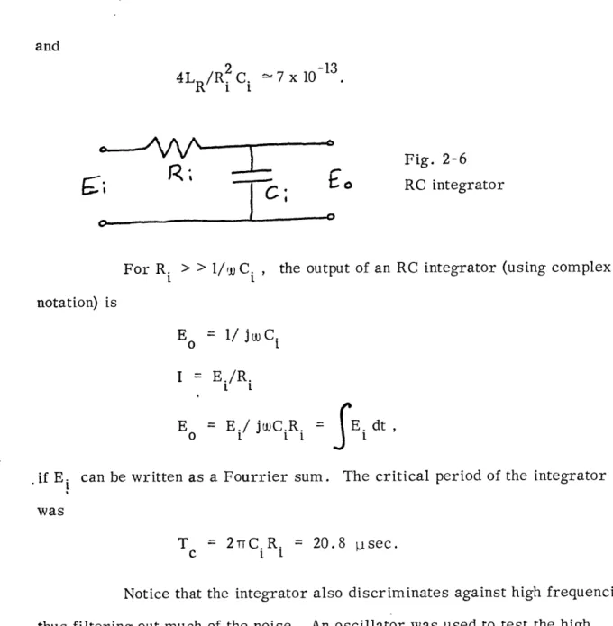
The Rogowski coil was connected to an RC integrator, for which

R. =330

,

and C.

Rogowski coil can be ignored, for it is only (approximately)

2 ₂

L R

-

ENA

19 nanohenries,

R

" o(length)

(2.24)

p sec:

-13

7x10

R;

C;

For R. > > 1/(C C , the outp notation) is

E

= 1/ jwuC.

O =

I = E./R.

E

= Ei/

juCiRi

can be written as a Fourrier sum.

T = 2rrC.R.

c It

Fig. 2-6

RC integrator

o

ut of an RC integrator (using complex

E. dt ,

The critical period of the integrator

= 20.8 tsec.

Notice that the integrator also discriminates against high frequencies, thus filtering out much of the noise. An oscillator was used to test the high frequency response of the integrator; it failed above 7 MHz.

Let Y be the attenuation of the integrator, Y = E /E.

O 1 = T/2rC.R. = T/ 20.8 .

Combining equations (2.26) and (2.25) gives

E

The current (equation 2.14) is

was

(2.26)

(2.27)

3 NV I = 94.2 x 10 (2.14) T Thus, I (amperes) = 1.03 x 104 E (volts). (2.28) This equation relates the current in the copper spools to the voltage output of the Rogowski coil/integrator circuit.

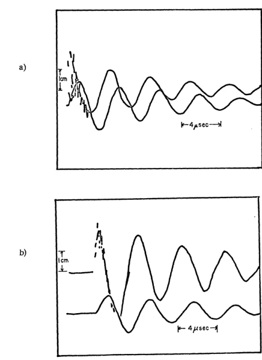
Typical records of Rogowski coil voltages are shown in figure 2-7 and photo 3. Unfortunately, the magnitude of the first integrated voltage peak is anomalous, for it fails the test

T/ 2

I dt = Q = NCoV.

0

Reference to the unintegrated voltages reveals there is a great deal of noise in the first half cycle. The low integrated first maximum must result from failure of the integrator to properly integrate through that noise.

Since good data for the first current maximum cannot be obtained directly from the recorded Rogowski coil output, we calculated I(max) from the recorded periods. We took T to be twice the interval between the first (positive) and second (negative) current maxima. (Sometimes, the first maxi-mum was very poorly defined; in those cases, the period was taken as twice the interval between the second and third current maxima.) I(max) is calculated from equation 2.14, using the measured values of T.

Figure 2-7 Some examples of Rogowski coil and integrator signals

(traced from oscillographs).

a) I Capacitor, 15 kV.

Upper trace: Rogowski coil output,

200 V/cm.

Lower trace: Integrator output, 20 V/cm.

b) 2 Capacitors, 17 kV.

Upper trace: Rogowski coil output,

200 V/cm. Lower trace: Integrator output, 50 V/cm.

2.2 Effects of the Pinch

2.21 Production of high pressures The magnetic pressure is

B2

P

-2p

The field produced by the current, I, in the copper spool is P° I

2rrr Thus,

P

2o

(2.29)

8r2 r

Substituting d = 2r and the value for I(max) in equation (2.14),

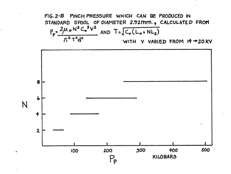
2 u N2 C2 V2 P(max) o o (2.30) 2 _Td or 2'2 P(max) = 5.66 N V P (2.31) d2T 2 p

Thrbughout this paper, the term "pinch pressure" refers to P in equation (2.31). P is a convenient quantity because it is easily evaluated from measured parameters, and it comes from equation (2.29), which is an exact expression for the magnetic pressure at the surface of the spool. However, except for the case of zero current penetration, equation (2.29) is not a rigorous expression for the pressure inside the spool. An exact calculation of the pressure

inside the spool is impossible because the radial variation of resistivity is not known. It is shown in appendix A4 that due to current penetration, the sample

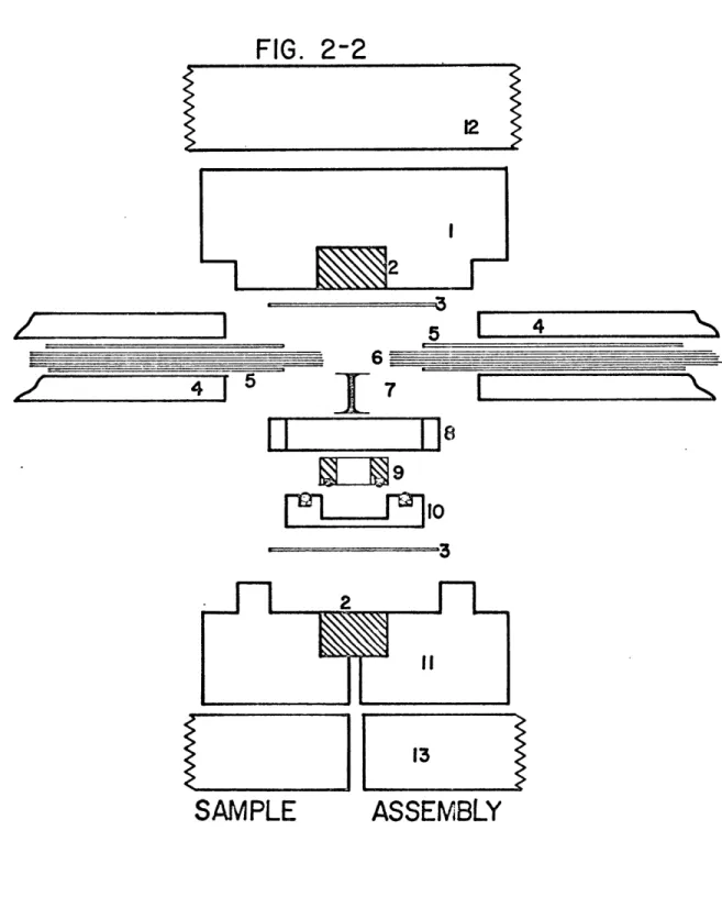
FIG. Z-

PINCH PRESURE

WH ICH

CAN BE PRODUCED IN

STANDARD

SPOOL

OF DIAMETER 2.92Tir.,

CALCULATED

FROM

p-

2oN

C

v

AND

T= CO(Lo NLq)

iaT

WITH

V

VARIED

FROM

I1420 KV

100

ZOO

Pp

300

Kil

o

KI LOBAR.,

500

41

The greatest value of P produced in a 2.92 mm diameter spool

was in shot DI. There N

=

8, and V= 16. The measured period was 6 Psec,

thus P

(from equation 2.31) was 300 kilobars. Figure 3-8 shows the

maxi-mum pressures obtainable in 2.92 mm diameter spools for various values of

N.

It is interesting to note the

spool becomes very small:

behavior of P as the radius of the

p

T

1

r

P

_P

_{r In}

r

This argument will fail, of course, because T will start to depend

strongly on the spool resistance when r gets very small. Specifitcally, Pp

will increase as shown above until

2 4L R C r r 2 D 2 o In -TC r

(2.32)

where p and . are the resistivity and length of the sample, C = NC , and

D is as defined in figure 2-4. Equation (2.32) is solved graphically on the next

page.

but

-3

-2

-I

.10

.o5

.oo

-2

The equality in equation (2.32) holds when r 10- mm. For -7

this value, L 12.5 x 10-7 h, T w 77 usec, and equation (2.31) yields 600 Megabars! Needless to say, this pressure is not usuable for studying effects in solids, since a spool of .02 mm diameter is too small to instrument.

Looking ahead to the next section, we can calculate the energy required to vaporize a .02mm diameter spool by multiplying the value given in figure 2-10 by 10-2/(2.92)2 . Doing so, and comparing the result with figure 2-9, shows that the discharge producing 600 Megabars will impart to the spool over 1000 times the energy required to vaporize it.

The precision with which P can be computed is given by

= 2 2A 2 ++ A2 (2.33)

V was usually read to .1 kV. The outside meter was calibrated with a Hewlit Packard VTM Model 412A and a Calibration Standard Corporation 1000:1 Precision High Voltage Divider. d was machined to ± .0005 inch, and T could usually be read to ± .2 psec. C was checked with a General Radio impedance

bridge to be ± 1 pf. For common values of V and T (15kV and 5 Usec), equation (2.33) becomes

P

= 10-2 x . '88 + 38 + 32 + 8 -. = .11 (2.34)

p

2.22 Melting of the copper spools

In experiments which produced pinch pressures greater than about 100 kilobars, the copper spools were usually completely destroyed. That is, except for the end-flanges, nothing of the spools could be recognized in the debris remaining in the guard ring after the experiment. The purpose of this

section is to calculate the rate at which energy is deposited in the spools, and to compare it with the heat content of the spools at elevated temperature. Appendix A2 reviews all the pertinent observational data in this area. The conclusions of the two sections agree very well.

The rate at which energy is deposited into the spools is given by R 12, where R5 is the resistance of the spools. R can be calculated from

the restivity p by means of the equation:

R = Pt (2.35)

s Ts (2r - s)

where , is the length of the spool, r is its radius, and s is the skin depth, given by

S Tp F,.TU.

A typical value of s is .2 mm.

to changes in

R

5 in equation (2.35) is relatively insensitive p, since

R

cr

P

1.

s 2

s

Equation (2.35) has been evaluated for two extremes of p, the normal value of

-8 -6

2 x 10 .- m and 10 f2 - m which Bennett et. al. (1964) obtained for the resistivity of liquid copper near vaporization in an exploding wire.

of Rs thus generated were 1.7 x 10

The extremes

D and 1.96 x 10

The energy absorbed by the sample is

Q(t')

_{R 1}

The current is

-Rt/L s 2

e

sin (2rrt/T) ,

Q(t')

=

t

'

0

+

2

T

L

T

e -Rt/L

8r

L

T

R

rt/T)

L

t

So that

2 = 12

I

=1

(2.36)

T

8rr I L (R /R)

o s -Rt'/L)

Q(t')

T (R /L +16r /T for t' = nT/2. Reducing further:

S1 2 Rs -Rt/L

Q

-SNC V2 ( I - eRtL) - (2.37)

o R

In equation (2.37), Rs is the resistance of the sample, and R is the total resistance of the circuit.

We can measure R from the decay of the current. According to equation (2.36), the amplitude ratio of the first and second current peaks (separated by T/2) is I1 RT/4L 2 or, 4L R = T log (I1/12) . (2.38)

R in equation (2.38) was computed by using equation (2.14) to calculate II and equation ( 2.28) to calculate 12. The data were taken from several shots in which V = 15 kV and the oscilloscope records were clear enough to allow all relevant quantities to be read to within 10%. The results are given on the next page:

shot

1

(units of 10

amps)

R (units of 10 -3

R (units of 10

)

21.9

10.9

8.76

26.4

8.67

9.2

For most cases, R is in the range 15

-4

of R =1.8 x 10

s

-3

+-7x10 f2

0

. Using a mean value

fall in the interval

Rs/R

(1.2 ± .4) x10-2

Figure 2-9 is a graph of

1

R

o

evaluated for

Rs/R

The copper spool shafts are heated according to the relation

T

Q/MC

where M is the mass of the spool hafts and C is the heat capacity of copper. For copper at STP, C =

.092 cal/gm-oC.

1/MC = 65.7

"C/cal.

Kelly (1960) gives the heat content of r.copper up to 2800 "K.

From

his data, the heat content (in gram calories) of the spool shafts is plotted in

figure 2-10. Added to it is the heat of vaporization of the shafts, computed

60

50

O

0

10

co

w

12O

W

-J

0

5

10

15

20

VOLTAGE

ON BANK

(kv)

Fig.

2-9

240

210

180

150

-J

0

O

a.

,)

,, 90

0

O

wJ

₆₈

I-z 60

O

T

30

26.3

25

100

500

1000

1500

2000

2500

25

TEMPERATURE

OC

Fig. 2-10

49

from the CRC Handbook value for copper. The values given in figure 2-10 lack

any pressure correction.

Comparison of figures 2-9 and 2-10 suggests that the spools will be

destroyed when four capacitors are employed at voltages greater than 17.4 kV.

This agrees very well with observation. It is also clear that joule heating

cannot vaporize the spools.

It is important to note that although the copper spool may be heated

to over 2000 C, the sample will not get hot during the time that the pinch is

applied. This is a consequence of the relatively long time scale of thermal

convection. The radial temperature distribution in a rod of uniform composition

is governed by the equation

d2T

1 dT

1 dT

2

r

dr

2

dt

dr

a

in which a = K/c Pm (K = _{thermal conductity, c} = _{specific heat, and pm}

mass density). The solutions to this equation are Bessel functions;

-k2 t

T =

AnJo(knr/

_{e n}

₊

To.

n

Let r be the sample diameter. We take the following boundary conditions:

T=0 for r<r , t=0

T = T for r r , t >0,

O O

so that

The values of A which satisfy equation (2.41) are given by Hildebrand (1962),

p. 231. The first ones are

A = -1.602 T A = 1.065 T k = 2.405 a/r0 k2 = 5.520 ai/r '

The values of a for the materials in the spools (ceramic or sample

material) were in the range .4 ±.3 cm/secK. Thus, k

is in the range 1.2 + .9

-1

sec 5. Therefore, the range of charcteristic times, even for these pessimistic

approximations, were

+ .1

1

t = .007 sec.

k - .004

The pinch pressure was only applied for about 10 u sec, thus, the

sample could not be heated by conduction during the time the pinch pressure was

applied. However, when thermal equilibrium was reached between the sample

and the spool, the sample may have become very hot. Some experimental

results pertinent to this subject are given in section 4.1.

III. EXPERIMENTAL INVESTIGATIONS

3.1 Quartz

3.11 High pressure data on quartz

It is well known that fused quartz can be irreversibly densified by

application of high pressure. However, the magnitude and cause of this effect

are still subjects of controversy; figure 3-1 is a compilation of most of the

published data.

The densification of quartz glass was first observed by Bridgman

and Simon (1953).

Using uniaxial compression, they measured the average

density of solid quartz discs after pressure was applied. Above a threashold

Cristiansen et. al. (1962) also employed unaxial stress on solid quartz discs.

They found a threashold of only 40 kilobars. MacKenzie (1963) reported a

threashold of about 60 kilobars. He employed solid samples in a belt

appara-tus; it turned out that the magnitude of the increase in refractive index, n,

de-pended on the material out of which the apparatus was constructed. MacKenzie

and Laforce (1963) and Saaka and MacKenzie (1969) used these results and a

rather dubious interpretation of the data of Christiansen and Roy and Cohen to

conclude that the densification of quartz is soley a function of shear stress, and

would not occur in a truly hydrostatic pressure chamber.

Cohen and Roy (1965) used a unaxial press to study densification of

ground fused quartz at various temperatures. It was found that elevated

tem-perature caused the densification to take place at lower pressure, and that

there was a maximum possible value of n for each temperature. They concluded

52

structure of the glass which is attained in a few minutes and then persists

in-definately at room temperature and atmospheric pressure." This conclusion

is directly opposed to that of MacKenzie. The indices of refraction observed

after quench from pressure were in a range ± .005 to

.008.

Roy and

Cohen proposed the hypothesis that the increase in density comes about by

rearrangement of basic structural units, most likely tetrahedral in shape.

Bridgman, Christiansen and MacKenzie measured densities.

How-ever, we have used the linear relationship between density and refractive index

(Cohen & Roy, 1962, MacKenzie, 1963) and the normal index of fused quartz

(1.460) to plot their data in figure 3-1 coordinates.

Wackerle (1962) has been the principal investigator of the effect of

shock waves on fused quartz. He found that below 98 kilobars the compression

was elastic. Material recovered from 250 kilobars was densified to 2.4

-2.5 gm/cm

(n = 1.580 to 1.650). At 500 kilobars, the recovered material was

ordinary amorphous quartz. Shock waves in crystalline quartz resulted in the

formation of ordinary glass at pressures of 300 to 600 kilobars (DeCarli and

Jameison, 1959). Therefore,

it

appears that permanent densification of quartz

It is not possible to predict whether pinch pressure can produce

high pressure crystalline polymorphs of quartz. Although coesite is stable

at only 21.5 kilobars (room temperature) (Bell & Boyd, 1968), it has never

been recovered from laboratory shock experiments on fused or crystalline

quartz. Traces of stishovite can be produced by only 75 kilobars in static

apparatus (Sclar et. al., 1963), and by much higher shock pressures in

cry-stalline quartz (DeCarli and Milton, 1965).

Both coesite and stishovite can

form in natural impact events (Chao et. al., 1960, Chao et. al., 1962). Since

a glass-like phase is formed as an intermediate stage in high pressure quartz

FIG.3-1 THE EFFECT OF PRESSURE ON THE INDEX OF REFRACTION OF FUSED SILICA, 250

~~BIB~~BIIIP

~

~

~

I

v, v

4

4

4

PRESSURE

(

KILOBARS)

0 COHEN & ROY , 1962

A BRIDGEMAN 8 SIMON, 1953 V MAC KENZIE, 1963 1.595 1.575 1.555 A z O 1.535 O 1.515 X W L1.4 95 O W 1.475 1.455

phase transitions (Dachille et. al., 1963, Chao, 1963), coesite or stishovite may

be produced during pinch experiments on fused quartz. If they are, they should

be recovered, since coesite is very stable at atmospheric pressure, even at

1400

_{C (Dachille et. al., 1963).}

_{Various accounts of the stability of stishovite}

have been reported

-

complete - reversion to glass in five minutes at 600

C

(Dachille et. al., 1963), vrs. partically no reversion in 8000 minutes at 600

C

(Skinner & Fahey, 1963).

We have subjected quartz glass to pinch pressures of 37 to 250

kilo-bars. Consideration of the preceding data leads us to seek answers to the

following questions:

1) How is the index of refraction of quartz glass related to pinch

pressure? Will an irreversible incrdase occur, as in static experiments, or

will there be no change, as in some shock experiments? Will the relatively

small amount of shear result in a lower index than in opposed anvil experiments?

What will the threashold pressure for densification be?

2) Can coesite or stishovite form under pinch conditions, where

the pressure is barely in their stability ranges, but of slightly longer duration

than in shock waves?

3) Can a pinch pressure scale be based on the change in n as a

function of P ?

p

3.12 Pinch experiments on fused quartz

Four experiments were done with powdered fused quartz; the grain

sizes were .061 to .044 mm. The powder was tapped into Imm holes drilled

through the axis of 4 and 6 mm diameter spools, as shown in figure 3-2a.

The spools were made from OFHC copper and molybdenum. The shots were

numbered GQI through GQ5, and the shot parameters are given in Appendix Al.

4 INCH1

FIG.

5 -Zb

I2

IYz

wcH

-.

040" DIAMi.

QUARTZ ROD

OR

POWDER

FIG. 3-2 a

I