HAL Id: hal-00317279
https://hal.archives-ouvertes.fr/hal-00317279
Submitted on 19 Mar 2004
HAL is a multi-disciplinary open access
archive for the deposit and dissemination of
sci-entific research documents, whether they are
pub-lished or not. The documents may come from
teaching and research institutions in France or
abroad, or from public or private research centers.
L’archive ouverte pluridisciplinaire HAL, est
destinée au dépôt et à la diffusion de documents
scientifiques de niveau recherche, publiés ou non,
émanant des établissements d’enseignement et de
recherche français ou étrangers, des laboratoires
publics ou privés.
magnetospheric states
M. A. Shukhtina, N. P. Dmitrieva, V. A. Sergeev
To cite this version:
M. A. Shukhtina, N. P. Dmitrieva, V. A. Sergeev. Quantitative magnetotail characteristics of different
magnetospheric states. Annales Geophysicae, European Geosciences Union, 2004, 22 (3),
pp.1019-1032. �hal-00317279�
SRef-ID: 1432-0576/ag/2004-22-1019 © European Geosciences Union 2004
Annales
Geophysicae
Quantitative magnetotail characteristics of different
magnetospheric states
M. A. Shukhtina1, N. P. Dmitrieva1, and V. A. Sergeev1
1V. A. Fock Institute of Physics, St.-Petersburg State University, St.-Petersburg, Russia
Received: 21 February 2003 – Revised: 21 July 2003 – Accepted: 21 August 2003 – Published: 19 March 2004
Abstract. Quantitative relationships allowing one to com-pute the lobe magnetic field, flaring angle and tail radius, and to evaluate magnetic flux based on solar wind/IMF pa-rameters and spacecraft position are obtained for the middle magnetotail, X=(−15, −35) RE, using 3.5 years of
simul-taneous Geotail and Wind spacecraft observations. For the first time it was done separately for different states of mag-netotail including the substorm onset (SO) epoch, the steady magnetospheric convection (SMC) and quiet periods (Q). In the explored distance range the magnetotail parameters ap-peared to be similar (within the error bar) for Q and SMC states, whereas at SO their values are considerably larger. In particular, the tail radius is larger by 1−3 REat substorm
on-set than during Q and SMC states, for which the radius value is close to previous magnetopause model values. The calcu-lated lobe magnetic flux value at substorm onset is ∼1 GWb, exceeding that at Q (SMC) states by ∼50%. The model mag-netic flux values at substorm onset and SMC show little de-pendence on the solar wind dynamic pressure and distance in the tail, so the magnetic flux value can serve as an important discriminator of the state of the middle magnetotail.
Key words. Magnetospheric physics (solar wind-magnetosphere-interactions, magnetotail, storms and substorms)
1 Introduction
Interaction of the Earth’s magnetic field with the solar wind plasma causes the bundles of magnetic field lines to extend in the anti-solar direction forming the magnetotail. To a large degree its properties are determined by the solar wind param-eters. Now a great amount of magnetic measurements cov-ering a wide range of solar wind/IMF conditions is available in different parts of magnetosphere. This allows one to con-struct statistical data-based magnetospheric models describ-Correspondence to: M. A. Shukhtina
(mshukht@geo.phys.spbu.ru)
ing the magnetospheric magnetic field for given external con-ditions, such as Tsyganenko (1996), Ostapenko and Maltsev (1997), Tsyganenko (2002). However, this approach is lim-ited and these statistical models are principally unable to ac-curately predict the magnetic field variability. The basic rea-son is that, besides the solar wind parameters, the magneto-spheric characteristics and dynamical evolution also depend on the previous evolution, as the magnetosphere can stay in different magnetospheric states. For example, during south-ward IMF the magnetosphere can either show large changes associated with substorm (passing through the growth phase, expansion and recovery phases, e.g. Russell and McPherron, 1973) or stay in the state of steady magnetospheric convec-tion (Sergeev et al., 1996). This variability is ignored in the aforementioned statistical magnetospheric models by their design.
There exist event-oriented models which give a snap-shot of the part of the magnetosphere sufficiently covered with spacecraft observations (see the models for the growth phase, e.g. Pulkkinen et al., 1991, or steady convection, Sergeev et al., 1996). However, due to poor statistics these models cannot describe reliably the global configuration and separate the effects of external variability from the consequences of internal processes.
A large amount of the works studying the substorm effects in the magnetosphere (following basic papers by Fairfield and Ness, 1970, Russell and McPherron, 1973, Caan et al., 1973, Fairfield et al., 1981, etc.) allowed one to understand many basic features of substorm phenomenon; however, they had either a qualitative character or had very localized sub-jects or the considered spatial domain. Summarizing, we still have no quantitative empirical model to describe the differ-ences of magnetospheric magnetic fields associated with dif-ferent magnetotail states.
A step toward such a model is done in our study where we construct the statistical models of basic magnetotail param-eters separately for three basic magnetospheric states. The quiet magnetotail (Q) is a natural background state with lit-tle electromagnetic interaction (and litlit-tle energy exchange)
between the solar wind and the magnetotail. The steady mag-netospheric convection (SMC) state is a basic state with in-tense interaction, in which the magnetosphere supports the plasma circulation in a steady-state fashion. Such a state is known to exist, but its magnetotail magnetic fields are rarely studied (most of the the existing information was summa-rized by Sergeev et al., 1996), so our task here is to ob-tain quantitative characteristics of this state and compare it to both the quiet state and the substorms.
The third state selected is the substorm onset (SO), the state just before the global energy dissipation starts explo-sively in the magnetotail. As compared to the later stages in-volving strong and complicated local perturbations, the mag-netospheric configuration at the end of the growth phase is still expected to keep the smooth magnetic field distribu-tion. At the same time, as a result of large-scale evolu-tion, this configuration may considerably deviate from back-ground properties, and our main interest will be to evaluate these differences in quantitative terms.
Our approach will be to construct the regression models for a few basic variables describing the magnetotail state, which can be observed or computed from simultaneous mea-surements in the tail and solar wind. Among them we choose the tail lobe magnetic field BL and the flaring angle α of
the tail magnetopause which characterizes the interaction be-tween the solar wind and the tail (and is computed from the force balance). These two parameters depend differently on the external factors. Following the southward IMF turning both considered parameters are known to increase, providing the lobe magnetic flux increase (Caan et al., 1973; Maezawa, 1975; Fairfield et al., 1981; Fairfield, 1985). On the other hand, the solar wind dynamic pressure (Pd) variations
influ-ence them differently: enhanced Pd increases the BLvalue
(Nakai et al., 1991; Fairfield and Jones, 1996; Tsyganenko, 2000), but decreases the flaring angle (Nakai et al., 1991; Petrinec and Russell, 1996). As a result, the use of either BL
or α is insufficient to describe the magnetospheric behavior, whereas their joint study helps to separate the effects of IMF and Pd and gives a more complete description of the
mag-netospheric system. Based on the obtained relations for α it is possible to calculate the tail radius RT. A great advantage
in knowing both parameters (BL and RT) is the possibility
to calculate the tail magnetic flux F, a fundamental global parameter of the magnetotail.
A number of previous studies treated statistically as a func-tion of distance and solar wind parameters either the lobe field variations (e.g. Behannon, 1968; Mihalov and Son-net, 1968; Sonnet et al., 1971; Slavin et al., 1985; Nakai et al., 1991; Fairfield and Jones, 1996; Borovsky, 1998; Tsyganenko, 2000), or the magnetopause shape and size (e.g. Sibeck et al., 1991; Roelof and Sibeck, 1993; Petrinec and Russell, 1996; Shue et al., 1997, 1998). The empir-ical models (Tsyganenko, 1996, 2002) use the predefined magnetopause which changes self-similarly in shape (chang-ing with the dynamic pressure but independent of the IMF, neglecting the well-known magnetopause flaring variations during substorms). Only Petrinec and Russell (1996)
(there-after referred to as PR96) considered both variables together and combined them to obtain the magnetic flux estimates. We expand their approach by using a more extended data set and by doing such analysis for different magnetotail states separately.
2 Data preparation and analysis 2.1 Data analysis and event selection
Our approach is based on the tail approximation (Birn, 1987), in which ∂/∂Z=O(1), By, Bz, ∂/∂X, ∂/∂Y =O(ε)
for ε2<<1, providing the conservation of one-dimensional pressure balance, which allows one to compute both the lobe magnetic field BL and the magnetopause flaring angle α.
This dictates the choice of the distance range (X<−15 RE)
in the tail where this approximation is valid.
The equivalent lobe magnetic field BLis computed from
the magnetic field and ion plasma parameters (n, Tp) in (or
near) the tail plasma sheet measured at the Geotail (GT) spacecraft as:
BL2/2µ0=B2/2µ0+n kT (1)
where T =1.14Tp, to take into account the electron
contribu-tions (assuming Tp/Te=7, e.g. Baumjohann, 1993). Based on computed BLand on the solar wind parameters observed
at Wind spacecraft (time-shifted to the Geotail location with
1t =(XGT−XW ind)/Vsw), the flaring angle α is calculated
from the pressure balance on the magnetopause as : 0.88Pdsin2α + Bsw2/2µ0+npk(Tisw+Tesw) = BL2/2µ0
, (2)
where Bsw is the interplanetary magnetic field, np and Tisw are the observed solar wind ion parameters, assuming
Tesw=Tisw. According to Newbury and Russell (1998), the
best approximation for the solar wind electron temperature is Tesw=1.41 ∗ 105◦K; the assumption Tesw=2Tisw is also
often used. We compared α values calculated according to Eq. (2) using these three approximations and found the dif-ference to be ≤0.1%, so our assumption does not greatly af-fect the results. The coefficient 0.88 gives the ratio of the magnetosheath pressure to solar wind dynamic pressure for high solar wind Mach numbers (Newtonian approximation, e.g. Spreiter et al., 1966). As α isolines in the lobes deviate from the X=const lines, the calculated α values correspond to spacecraft position and should further be recalculated to the corresponding magnetopause coordinates X∗ (see Sect.
2.3).
We used data between January 1995 and April 1998 when the Geotail spacecraft was in the magnetotail at X<−15 RE
and |Y |<15 RE. We used Geotail magnetic field and ion
plasma moments available from the DARTS database with 12-s time resolution, computed the BLvalues, and then
aver-aged them over 6 min to obtain the final BL. Wind magnetic
and plasma data from the solar wind with ∼1-min resolu-tion taken from CDAWeb were also averaged over 6 min af-ter being shifted in time. The following input variables were selected in our model:
(1) The solar wind dynamic pressure Pd=1.94 ∗
10−6npVsw2 (assuming 4% helium content as in
Tsyga-nenko, 1996), with Pdin nPa, proton number density np in
cm−3, Vsw in km/s. This is the basic parameter controlling
the tail magnetic field (e.g. Fairfield and Jones, 1996), as well as the size of magnetotail (PR96).
(2) The “dayside merging” electric field
Em=Vsw(Bysw2+Bzsw2 )1/2sin32/2 (where 2 is the IMF clock angle in Y Z plane). The power law index 3 was chosen as it typically gives the best correlation with the cross-polar cap potential drop (e.g. Boyle et al., 1997; Eriksson et al., 2000). It was taken to be averaged over the 60 min preceding the observation in accordance with the results of Bargatze et al. (1985), who revealed the 60-min interval presumably corresponding to the accumulation time of the magnetic flux in the tail. Though the SMC mode is a direct driven one and is assumed to correspond to the 20-min time scale according to Bargatze et al. (1985), we also used the 60-min averaging interval for the SMC events for joint formal description of all states. Note that the choice of the averaging interval is not crucial for the SMC regime, as the SMC data set is characterized by stable solar wind/IMF conditions.
(3) Geotail position in the magnetosphere. We used alter-natively either the X coordinate, or the geocentric distance in the equatorial plane R=(X2+Y2)1/2(which is ∼(X2+Y2+ Z2)1/2for Geotail since Z∼0). The R-dependence is consid-ered because lines of constant BLclosely follow the R=const
lines (e.g. Fairfield and Jones, 1996; Tsyganenko, 2000). The
X-dependence was considered because the magnetopause (characterized by the flaring angle) is supposed to be axisym-metric, with the symmetry axis coinciding with the X axis; besides, we compare our results with the results of PR96 and other magnetopause models, where the X-dependence of the flaring angle and magnetotail radius were used.
All data is presented in a GSM coordinate system. So-lar wind and magnetotail data are used together with ground indices and high-latitude magnetograms to select the events of different kind. Ground PC index with 5-min resolution from Thule was taken (for some periods when Thule data missed we used 1-min PC-index from Vostok station). SYM and AE indices with a 1-min resolution, together with the PC index were used to control the geoefficiency of solar wind structures detected by Wind and to select the magnetospheric state. We also used magnetograms from ground magnetic stations in three longitudinal sectors (IMAGE, CANOPUS, 210 MM) to check the substorm onsets.
To categorize the magnetospheric states we used the fol-lowing formal criteria:
Quiet state (Q) We required Em <0.5 mV/m (also
PC<0.5 mV/m and AE<50 nT) at the time of observation and at least 2- h before. The 2 h-long interval was chosen to avoid the effect of previous substorm activity, as it exceeds the time interval between substorm onset and the end of the recovery phase (about ∼1.5 h according to Fairfield et al., 1981, and Baker et al., 1994a). 2172 of the 6- min-long
sam-ples from 48 events have been identified as belonging to the Q data set according to these criteria.
Steady Magnetospheric Convection (SMC) We required a substantial external driving (Em>0.5 mV/m, PC follows Emvariations) without substorms during the preceding hour (both lobe field variations and AE index, as well as auroral zone magnetograms were checked). The lobe field variations associated with solar wind Pdvariations were allowed if they
were within 5% of prediction by the statistical relationship from Fairfield and Jones (1996). 1412 6-min-long samples grouped in 53 events have been identified for this SMC data set.
Substorm onset (SO) As different from many previous studies, we base the onset definition primarily on the behav-ior of the lobe magnetic field. Namely, we looked through high-resolution data plots and visually searched for the iso-lated sharp BL decrease, usually accompanied by a sharp BZ increase/decrease at Geotail. It was required that
cor-responding negative magnetic bays in the H component on the night-side auroral stations or in the AL index with am-plitude >100 nT were observed. By the name “isolated” we mean that the lobe field BLhas recovered well after the
previous substorm. Although multiple substorm intensifica-tions are well known (multiple-onset substorms), we hope such an approach allowed us to select the situations when the magnetotail was close to the onset of global instabil-ity (Baker et al., 1999); this is somewhat similar to the de-scription of the “main onset” by Hsu and McPherron (1998). Substorms inside the storm periods (registered >2 h after the storm main phase commencement and/or corresponding to SYM<−25 nT) were excluded. With these criteria we se-lected 132 well-defined substorm onsets, thus the SO data set contains 132 6-min-long samples (a single sample for ev-ery event). Ninety-five out of 132 onsets were preceded by the distinct BLgrowth, 34 were not, and for 3 substorms we
had gaps in the Geotail data for the preceding time interval. Average characteristics of these data sets are presented in Table 1.
2.2 Regression model for the lobe magnetic field and flar-ing angle
Our output variables are BLand α calculated from Eqs. (1)
and (2). Our input variables are the solar wind dynamic pres-sure Pd, the time-averaged dayside merging rate Em, and the
spacecraft position in the magnetotail (alternatively R or X, sharing the same functional form). The correlation coeffi-cients between different input parameters for each data set (given in Table 1) indicate that they can be considered inde-pendent in all cases, except for the pairs R and Em, X and Emin the SMC data set. Further, we checked to what extent
the outputs BLand α may be considered as independent
vari-ables. As α is calculated from Eq. (2) using BL, one may
sug-gest that the two quantities are highly correlated. In fact, the correlation coefficients between BLand sin2αpresented in
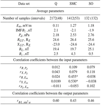
Table 1. Characteristics of different magnetospheric states.
Data set Q SMC SO
Average parameters
Number of samples (intervals) 2172(48) 1412(53) 132 (132) Em, mV/m 0.11 1.27 1.18 IMFBz, nT 2.1 -2.1 -1.9 Pd, nPa 2.18 2.53 2.76 RGT, RE 24.6 26.4 25.6 XGT, RE -23.0 -24.6 -24.4 BL, nT 19.4 19.7 25.1 Bz, nT 2.5 4.3 0.5
Correlation coefficients between the input parameters rR,Pd 0.012 0.109 0.079
rX,Pd 0.043 0.079 0.118
rR,Em 0.024 0.455* -0.038
rX,Em 0.0189 0.530* −0.038
rPd,Em −0.011 −0.053 0.102
Correlation coefficients between the output parameters rBL,sin2α 0.60 0.43 0.46
their joint study gives more information than if they were an-alyzed separately.
The functional forms for BLand α were chosen based on
the results of previous works. According to Fairfield and Jones (1996), Mihalov and Sonnet (1968), BL is well
de-scribed by a power function of R. Though at large distances (tailward of ∼100 RE)the BLvalue should approach a
con-stant (Slavin et al., 1985), it is unimportant for the R range considered, so, unlike Fairfield and Jones (1996), we did not include a free term into the R-dependence. The BL
depen-dence on Pd was well described by a power law (Fairfield
and Jones, 1996; Borovsky, 1998). The BLdependence on Em(not considered in the previous works) was assumed
ex-ponential: for Em=0 the corresponding multiplier becomes
1 and the dependence is linear for small Em values, which
looks reasonable. Therefore, the BLmodel is presented as BL=a1Pda2Ra3exp(a4Em), (3a)
BL=A1PdA2XA3exp(A4Em). (3b)
The exponential flaring angle dependence on R and X was chosen based on the results of PR96, Nakai et al. (1991), while its Pd-dependence was well presented by a power
func-tion. The Em-dependence of sin2αis chosen at Eq. (3). This
gives
sin2α = b1Pdb2exp(b3R + b4Em), (4a)
sin2α = B1PdB2exp(B3X + B4Em). (4b)
To solve for Eqs. (3) and (4) we followed PR96 and took the logarithm of both sides of Eqs. (3), (4), obtaining two
Table 2. Regression and correlation coefficients obtained from the
regression analysis.
Lobe field BLmodel Q SMC Substorm onset
a1 195.4 138.9 192.7 a2 0.336 0.268 0.275 a3 −0.8059 −0.680 −0.739 a4 −0.0315 0.027 0.0631 r 0.923 0.781 0.927 rPd 0.607 0.649 0.556 rR 0.719 0.429 0.666 rEm 0.016 −0.271 0.257
Flaring angle α model
b1 0.5753 0.5881 0.7303 b2 −0.2000 −0.2664 −0.4175 b3 −0.0783 −0.0749 −0.0658 b4 −0.1826 −0.0313 0.0843 r 0.889 0.760 0.891 rPd 0.178 0.253 0.455 rR 0.838 0.655 0.802 rEm 0.018 0.279 0.070
r is the multiple correlation coefficient; rPd, rRand rEm are partial correlation coefficients with variations of Pd, R or Em.
linear systems for unknown coefficients a1, a2, a3, a4 and
b1, b2, b3, b4 (A1, A2, A3, A4 and B1, B2, B3, B4). The
obtained coefficients a1– a4, b1– b4are presented in Table 2
(see also Table 3 for the rest coefficients).
The results in Table 2 confirm that the most important fac-tors controlling both BLand α values are the spacecraft
geo-centric distance R and solar wind dynamic pressure Pd. For
the BL parameter the partial correlation coefficients
corre-sponding to R and Pd are high (∼0.6–0.7, except rR=0.429
for SMC) and close to each other. For the α parameter
rR>rPd, rPd>>rEm (the latter relation is violated for the
SMC state, see below). Thus R- and Pd-influence on BLare
of the same order, while the flaring angle is more affected by
R.
The influence of the dayside merging rate (Em) is less
im-portant, though more complicated to understand. Its negli-gible contribution during the quiet periods is expected. If we take a4=b4=0 for the Q data set, the multiple correlation
coefficients will change by <0.1% and variations of regres-sion coefficients are also very small. Thereafter, we neglect this dependence for the quiet state data set (new coefficients are given in Table 3). In the SO data set rEm=0.257 for the
BLparameter, so the influence of Emis not large but should
be taken into account. The α dependence on Em is small
(rEm=0.07); its exclusion reduces the multiple correlation
coefficient insignificantly (from 0.891 to 0.887) and changes the b1value by ∼10% from 0.73 to 0.81. We keep the Em
-dependence in the final model for both BLand α at substorm
onset.
The study of Eminfluence on BLand α for the SMC state
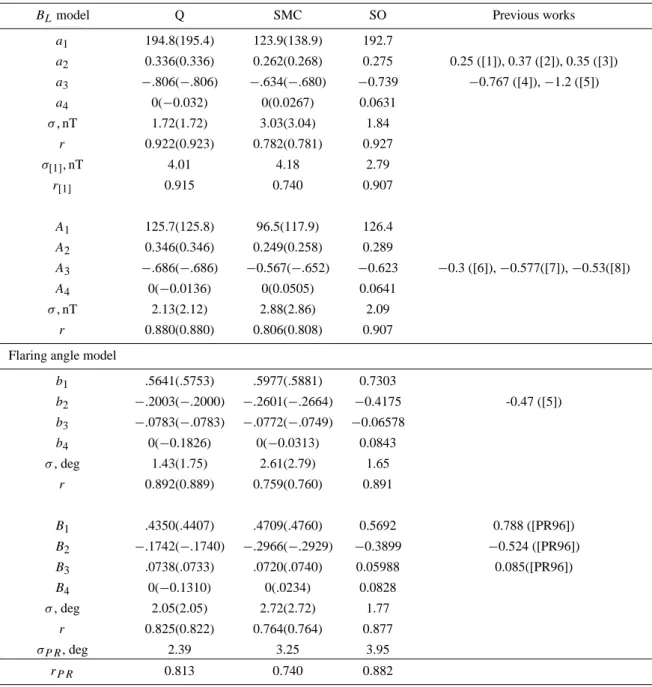
Table 3. Final (versus initial) regression model.
BLmodel Q SMC SO Previous works
a1 194.8(195.4) 123.9(138.9) 192.7 a2 0.336(0.336) 0.262(0.268) 0.275 0.25 ([1]), 0.37 ([2]), 0.35 ([3]) a3 −.806(−.806) −.634(−.680) −0.739 −0.767 ([4]), −1.2 ([5]) a4 0(−0.032) 0(0.0267) 0.0631 σ, nT 1.72(1.72) 3.03(3.04) 1.84 r 0.922(0.923) 0.782(0.781) 0.927 σ[1], nT 4.01 4.18 2.79 r[1] 0.915 0.740 0.907 A1 125.7(125.8) 96.5(117.9) 126.4 A2 0.346(0.346) 0.249(0.258) 0.289 A3 −.686(−.686) −0.567(−.652) −0.623 −0.3 ([6]), −0.577([7]), −0.53([8]) A4 0(−0.0136) 0(0.0505) 0.0641 σ, nT 2.13(2.12) 2.88(2.86) 2.09 r 0.880(0.880) 0.806(0.808) 0.907 Flaring angle model
b1 .5641(.5753) .5977(.5881) 0.7303 b2 −.2003(−.2000) −.2601(−.2664) −0.4175 -0.47 ([5]) b3 −.0783(−.0783) −.0772(−.0749) −0.06578 b4 0(−0.1826) 0(−0.0313) 0.0843 σ, deg 1.43(1.75) 2.61(2.79) 1.65 r 0.892(0.889) 0.759(0.760) 0.891 B1 .4350(.4407) .4709(.4760) 0.5692 0.788 ([PR96]) B2 −.1742(−.1740) −.2966(−.2929) −0.3899 −0.524 ([PR96]) B3 .0738(.0733) .0720(.0740) 0.05988 0.085([PR96]) B4 0(−0.1310) 0(.0234) 0.0828 σ, deg 2.05(2.05) 2.72(2.72) 1.77 r 0.825(0.822) 0.764(0.764) 0.877 σP R, deg 2.39 3.25 3.95 rP R 0.813 0.740 0.882
The values in parentheses correspond to the full regression model (including the Em-dependence); σ is the standard
deviation; σ[1], r[1], σP R, rP Rare the standard deviation and correlation coefficient given by [1] and PR96
correspond-ingly. [1] Fairfield and Jones (1996); [2] Borovsky (1998); [3] Tsyganenko (2000); [4] Mihalov and Sonnet (1968); [5] Nakai et al. (1991); [6] Behannon (1968); [7] Sonnet et al. (1971); [8] Slavin et al. (1985).
Em(X and Em) in this data set (marked by a star in Table 1).
Anyhow, the regression coefficients a4, b4, B4,
characteriz-ing the Em contribution for the SMC data set are less than
one half of the corresponding coefficients for the substorm data set (whereas the values of A4 are comparable for two
states), see Table 3. Besides, the coefficients a4 (0.0267)
and A4(0.0505), as well as b4(−0.0313) and B4(0.0234)
strongly differ from each other, though for independent input parameters the relations a4∼A4, b4∼B4are expected (which
is true for the SO array). These considerations show that
the regression coefficients describing the Em-dependence for
SMC state are unstable and definitely are not reliable with the data set we have. Therefore, we decided to omit this depen-dence from the final model (although we do not claim that such dependence does not exist). The regression and correla-tion coefficients for the modified final models are presented in Table 3.
It follows from Table 3 that both BLand α are slightly
bet-ter described by using R as an input paramebet-ter (correlation coefficients are slightly higher, and the standard deviation
slightly smaller than for X) for Q and SO, while X is a more preferable input for the SMC data set (except the α standard deviation behavior). Generally, both R and X give high (ap-proximately the same) correlation coefficients.
The final model is given by expressions (3, 4) with the coefficients from Table 3. Below we rewrite the final regres-sion expresregres-sions for each data set in the more convenient form by normalizing the input variables to their average values:
Quiet-time data set
BL=19.8(Pd/2.5)0.336(R/25)−0.806
(5a)
α =arcsin((0.4696(Pd/2.5)−0.200.1423R/25)1/2)
Steady convection data set
BL=20.5(Pd/2.5)0.262(R/25)−0.634
(5b)
α =arcsin((0.4712(Pd/2.5)−0.260.1459R/25)1/2)
Substorm onset data set
BL=23.0(Pd/2.5)0.275(R/25)−0.7391.085Em/1.3
(5c)
α =arcsin((0.4982(Pd/2.5)−0.420.193R/25 1.1158Em/1.3)1/2)
or, with X-variable: Quiet BL=19.0(Pd/2.5)0.346(|X|/25)−0.686 (6a) α =arcsin((0.371(Pd/2.5)−0.17420.1580|X|/25)1/2) SMC BL=19.5(Pd/2.5)0.249(|X|/25)−0.567 (6b) α =arcsin((0.3588(Pd/2.5)−0.29660.1653|X|/25)1/2) Substorm onset BL=22.2(Pd/2.5)0.289(|X|/25)−0.6231.087Em/1.3 (6c) α =arcsin((0.3982(Pd/2.5)−0.38990.2238|X|/25 1.1136Em/1.3)1/2)
2.3 Magnetotail radius calculation
The model expressions for the flaring angle α specify the tilt of axis-symmetric boundary (magnetopause) as a function of distance. Since tan α=dRT/dx(where RT is the tail radius),
it can be formally integrated over [0, X] to obtain the spatial variation of the tail radius for each data set as
RT(X) = RT0+
X Z
0
tanα(x) dx, (7)
where RT0is some initial value of the tail radius, hereafter
supposed to be taken at the terminator (X=0). Integration of (7) using (4b) gives:
RT(X) = RT0−
2/B3(arcsin(C exp(0.5B3X)) −arcsin(C)), (8)
where C=(B1PdB2exp(B4Em))1/2, and B1, B2, B3, B4
coef-ficients are given in Table 3.
Following PR96, we ignore the RT0 dependence on the
IMF, and use their formula
RT0=14.63(Pd/2.1)−1/6 (9)
The choice of this RT0 model will be later discussed and
compared with other versions in Sect. 3.2.
Now we should take into account that the lines BL=const
and α=const approximately correspond to magnetopause normals near the magnetopause, whereas BL isolines
fol-low the lines X=const in the central part of the tail. There-fore (see Figure 1), the X value at Geotail position should be replaced with some new X* value at the magnetopause where the BLvalue is the same. In the region of the tail
ap-proximation this correction is small and with simple geom-etry of BL=const lines we can use it as X∗=X−1X, where 1X=(RT−(Y2+Z2)1/2)sin α cos α, where X, Y, Z are the
coordinates of the observation point. Following PR96, with the corrected coordinates we can solve again the regression problem (finding new coefficients B1∗, B2∗, B3∗, (B4∗for SO; Eq. 4b), calculate the new RT(X∗) function according to
Eq. (8), and so on. Similar to PR96 we found the iteration procedure to converge quickly (the solution became stable already on the second-third iteration). The resulting regres-sion models for the tail radius are given in Table 4.
3 Discussion
3.1 The pressure balance and its violations
Simple pressure balance in the magnetosphere and on the magnetopause are the basic assumptions of this work. The validity of the pressure balance assumption in the magne-tosphere was explored theoretically (e.g. Rich et al., 1972; Birn, 1987) and checked experimentally (Fairfield et al.,
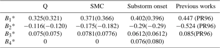
Table 4. Regression models for the tail radius using the terminator models from PR96 and from Shue et al. (1998) (the latter given in
parentheses).
Q SMC Substorm onset Previous works B1* 0.325(0.321) 0.371(0.366) 0.402(0.396) 0.447 (PR96)
B2* −0.116(−0.120) −0.175(−0.182) −0.29(−0.29) −0.524 (PR96)
B3* 0.075(0.075) 0.0781(0.0776) 0.0612(0.0612) 0.085(PR96)
B4* 0 0 0.076(0.080)
1981; Baumjohann et al., 1990; Petrukovich et al., 1999). It was shown that in general vertical balance exists in the magnetotail tailward of X∼−15 RE, though there are some
exceptions. For example, the 1-D balance may be violated in flux-rope-like structures (plasmoids and Traveling Compres-sion Regions, TCRs, e.g. Slavin et al., 1984). Such struc-tures, which are several minutes long and associated with a bipolar Bz-variation, are often observed close to substorm
onset (e.g. Maezawa, 1975). Another kind of anomalous event is reported by Petrukovich et al. (1999), who observed 3 cases of long (≥10 min) pressure pulses in the equatorial plasma sheet not seen in the tail lobe at the end of the sub-storm growth phase. Such rare observations were interpreted as a result of a collision of earthward and tailward flows in the plasma sheet, leading to the local plasma sheet thicken-ing. We took care to avoid such problems by inspecting Geo-tail data with a 2-min resolution. When such pressure peaks were found before substorm onsets, the events were “cut” (in 2 out of 132 selected substorms the BLvalue after or before
the pulse was taken) or discarded (for pulses longer than 5– 10 min).
The pressure balance along the magnetopause normal was demonstrated experimentally in PR96 (their Fig. 3). The va-lidity of this assumption is indirectly supported by a good coincidence of the magnetopause shape obtained in PR96 (where the pressure balance was a principal assumption like in our Sect. 2.3), with the statistics of observed magne-topause positions (Safrankova et al., 2002; Yang et al., 2002). 3.2 Comparison of BL, α and RT models with previous
re-sults
BLdependence on the geocentric distance R (or X coordi-nate), Pd, IMF and some other parameters was previously
studied by Behannon (1968), Mihalov and Sonnet (1968), Sonnet et al. (1971), Slavin et al. (1985), Nakai et al. (1991), Fairfield and Jones (1996), Borovsky (1998), Tsyganenko (2000). According to Table 3 the power indices describing the BL dependence on Pd (a2, A2)and R/X (a3/A3), on
average correspond well to previous results, except Behan-non (1968) for A3 and Nakai et al. (1991) for a3. The
lat-ter discrepancy is due to the different distance range (10 RE,
22 RE), analyzed in Nakai et al. (1991) (see discussion in
Fairfield and Jones, 1996). The Behannon (1968) A3value
is underestimated as compared to values obtained in all pre-vious works.
The agreement of our α model with previous results is not as good. On average, our α values show a weaker depen-dence on the distance and Pd than in Nakai et al. (1991),
PR96. The discrepancy of B3 values could be partly due
to the different X range (−10 RE, −22 RE) used in these
studies. As for the dynamic pressure dependence, the b2, B2
quantities differ significantly for different states, being much larger (and closer to the previous results) for the substorm data set than for the Q and SMC ones.
The IMF (Em) influence on the tail parameters cannot be
directly compared with other works, as they used other func-tions describing IMF contribution and also, this influence is of the second order of magnitude as compared to the influ-ence by R and Pd. However, we can compare BLand α
val-ues calculated with our model (Eqs. 5 and 6 and Table 3) with the expressions from Fairfield and Jones (1996) and PR96 (including their IMF-dependent terms) for our Q, SMC and SO data sets. These results are also presented in Table 3. Our correlation coefficients are, on average, slightly (by ∼1−3%) higher than those given by the models considered. However, the standard deviations in the previous models (Fairfield and Jones, 1996, PR96) are notably (sometimes more than twice) larger due to systematic differences in our three data sets (see Sect. 3.3).
When calculating the tail radius, some approximations were made, particularly, (a) we used a simplified procedure to compute the corresponding magnetopause X∗coordinate, and (b) we extrapolated the tail radius model (based on ob-servations made at X<−15 RE)until the terminator when
using Eq. (8). Therefore, the results for the tail radius re-quire a careful comparison with existing observation-based magnetopause models.
There is still a choice in selection of the terminator mag-netopause model. We used the simple model (Eq. 9) from PR96 ignoring the IMF-dependence of RT0, whereas Shue
et al. (1998) included the IMF effects together with dynamic pressure dependence. To check the validity of our choice we included the additional input parameter, 6-min average IMFBz, into our data sets, and repeated the iterative
proce-dure for both variants of the terminator model. The resulting coefficients describing the magnetopause shape (see Table 4) practically coincide for two terminator models tried, so the choice of either of these models is justified.
We also checked the influence of the assumed α isolines’ shape on the obtained RT value. It turned out that this shape
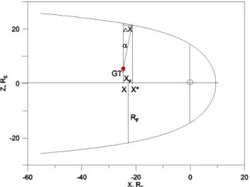
Fig. 1. The scheme presenting the geometry of Geotail
measure-ments for the day–night meridian. X is the Geotail position, X∗– the magnetopause coordinate, corresponding to the same BL/α val-ues, XF=0.5(X+X∗)and RT(XF)=0.5(RT(X)+RT(X∗))– the
quantities used when calculating the tail magnetic flux.
variant with circular symmetry of isolines (Fig. 1) somewhat better agrees with previous magnetopause models.
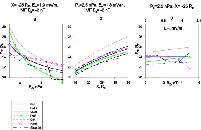
Figures 2a–c demonstrate the RT dependence on the
in-puts Pd, X, and Em for the present model compared with
previous ones, with other input parameters having their fixed average values. Note that other models use the IMF Bz
in-put instead of Em, and the relationship between these two
variables may vary. In Figs. 2a and b Em and Bz have
their average values for SO and SMC (1.3 mV/m and -2 nT), whereas in Fig. 2c the Bz value is calculated from Em
as-suming Vsw=400 km/s, 2=π , i.e. IMF By=0. According
to Fig. 2 our Q and SMC RT values everywhere lie
be-tween those given by other models (PR96, Sibeck et al., 1991 (S91); Roelof and Sibeck, 1993 (RS93); Shue et al., 1998), with the largest discrepancy (∼2 RE)being observed
with PR96 for Pd=6 nPa and with RS93 for IMF Bz=−5 nT.
Two dashed curves in Fig. 2b showing the empirical mag-netopause for dynamic pressure values bracketing our aver-age value (2.5 nPa) according to Sibeck et al. (1991) also have our Q and SMC curves between them. Such compar-isons allow us to be sure that numerically our magnetopause model has a good agreement with observed magnetopause positions, at least in the input parameters range near their av-erage values, where most of the empirical data points come from. The SO magnetotail models differ significantly from the empirical models and from our Q, SMC models, which is discussed below.
3.3 Magnetotail parameters in different dynamical states We have already noticed the large differences between the magnetotail parameters at substorm onset and in the dynam-ically equilibrium states (quiet and steady convection); now we discuss these differences in quantitative terms. We first
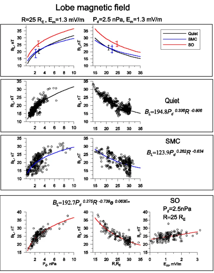
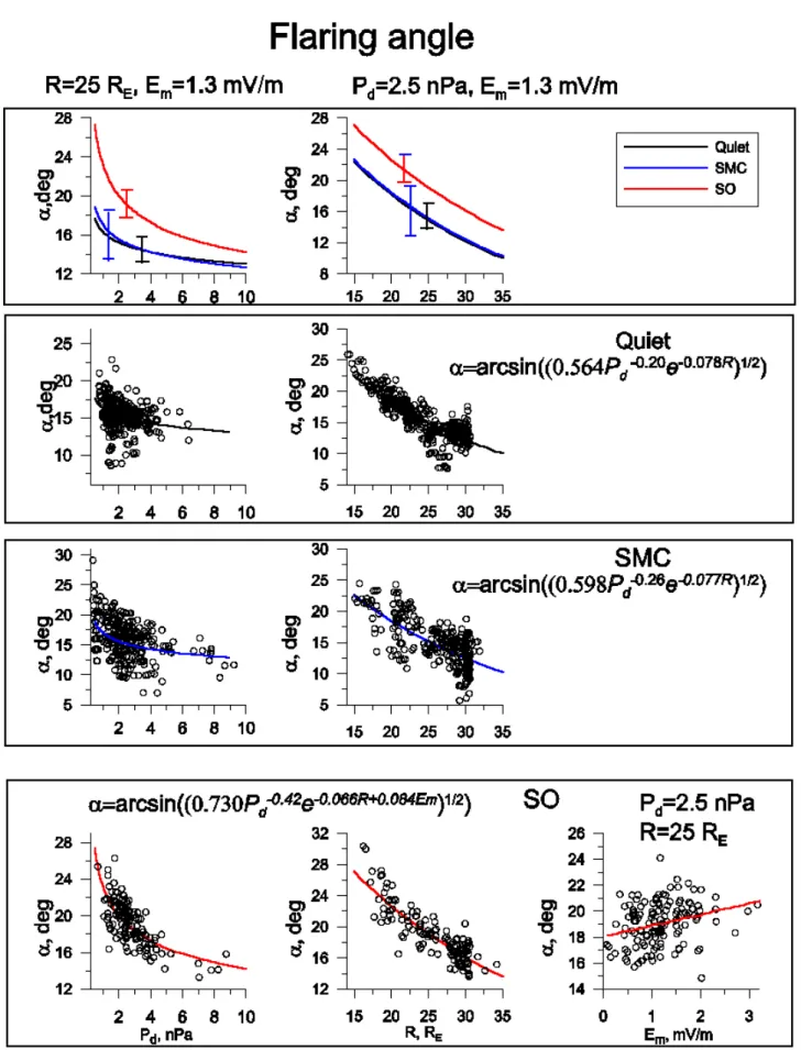
analyze the behavior of basic output variables, the lobe field and tail flaring angle, which is given by the coefficients in Table 3 and is illustrated in Figs. 3 and 4. Here we show the partial contributions of variations related to the distance (R), solar wind pressure (Pd) (and the Em-variation, only for
substorm data set). The top panel in each of Figs. 3 and 4 shows the variations in our Q, SMC, SO models (with other parameters fixed to their average values), with the error bars showing the standard deviations in each data set. The remain-ing plots illustrate each of these three models, as well as the scattering of data points. To produce these plots (to suppress the scatter due to variations of other input variables), the BL
and α values in each point were corrected according to the regression model (with the values of other variables reduced to their average values given in Table 1).
We emphasize that the scatter in BL(R), BL(Pd), α(R)
plots is small (corresponding partial correlations in Table 2 are high) for all states, so these dependencies are well de-fined, especially for Q and SO states. The α(Pd) plot is
characterized by substantially larger scatter. Finally, the Em
-dependence of BL is characterized by small (0.26) partial
correlation coefficient, whereas for α(Em) dependence the
correlation is negligible (0.07).
The next thing to emphasize is that the BL and α-values
for the SMC and Q data sets taken at the same distance and with the same solar wind dynamic pressure practically coin-cide within the error bars. The scatter for the SMC data set is larger, but the average behavior is well defined. In a case study of ISEE-1 observations at X=−20 RE during a steady
convection event, Sergeev and Lennartsson (1988) reported that the observed BL values for Q and SMC states were
19 nT and (18–22) nT correspondingly, whereas at substorm onset they exceeded 25 nT. According to our model, BL
values for Pd=1.5 nPa, R=20 RE, Em=(0.95−2.4) mV/m
(as in Sergeev and Lennartsson, 1988) are 19.6 nT(Q), 20.6 nT(SMC) and (25.0–27.4) nT (SO), in good agreement with these observations.
The third important feature is that the magnetotail at sub-storm onset has a well-defined state (parameters in Figs. 3 and 4 display a relatively low scatter), and its parameters are distinctly different from the Q, SMC data sets, with the dif-ference being larger than the error bar and larger than the difference between the Q and SMC models. Although the increase in the tail lobe field and flaring angle is well ex-pected from previous experience, this is the first quantitative model allowing one to compute the amount of tail lobe mag-netic field (and magmag-netic flux) increase prepared just before the onset of explosive large-scale tail instability (e.g. Baker et al., 1999) at different external conditions.
Maezawa (1975) studied experimentally the tail radius increase during the substorm growth phase. According to his estimates, the inferred RT increase in the X range
(−30, −70) RE during the growth phase is between 0.5 RE
and 4 RE, on average, being 1–2 RE, which agrees with the
difference between SO and Q, SMC RT values shown in our
Fig. 2. Magnetotail radius dependence on Pd, X, Em/Bzfor the present model compared with previous models.
3.4 Magnetotail magnetic flux variations
Having obtained the functions describing both the lobe mag-netic field and tail radius variations, we may estimate the tail magnetic flux (considering one tail lobe) as
F = BLπ RT2/2 (10) When calculating this parameter, one should take into ac-count the presumed circular geometry of BL=const lines. In
our approximation, for BL (referred to the coordinate X)
we determine X∗=X−1X, compute XF=0.5(X+X∗)(as in
Sect. 2.3, Fig. 1), calculate RT(XF)=0.5(RT(X)+RT(X∗))
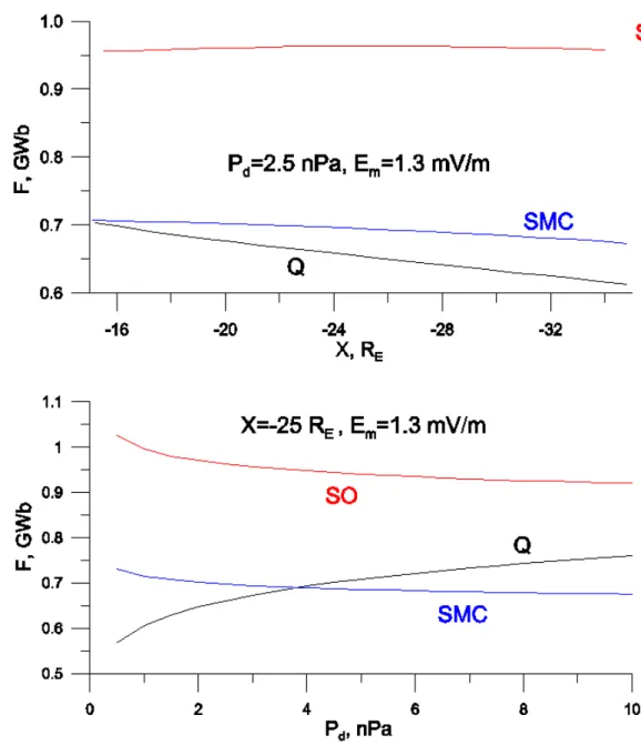
according to Eqs. (8) and (9) and Table 4, and use this value when computing Eq. (10). The results are presented in Fig. 5. Surprisingly, the so-computed F values have almost no de-pendence on the distance in the tail, as well as on the dy-namic pressure for the states with the strong coupling (sub-storms and SMC). In that sense the F value itself is a well-defined global parameter which could be considered as the global state variable for the magnetotail. According to this figure, the value of the tail magnetic flux at substorm on-set is about 1 GWb, exceeding that corresponding to Q state by 30–60% depending on Pd and X values. The SMC flux
value (∼0.7 GWb) coincides with the corresponding Q value within ∼15%.
There were a few previous estimates of this quantity. In a similar manner Petrinec and Russell (1996) calculated the tail magnetic flux for several time intervals. They com-puted the tail radius from their model and used the BL
value just measured by ISEE2 spacecraft in the tail lobe (ne-glecting the plasma sheet existence). They concluded that tailward of 15 RE the flux level dividing magnetotail states
both followed and not followed by a substorm onset is 1.0– 1.4 GWb, somewhat larger than our estimate ∼0.8 GWb. In their CDAW9 case study Baker et al. (1994b) estimated the polar cap size variation during the substorm growth phase; it corresponds to the polar cap magnetic flux ∼0.8 GWb at the beginning of the substorm growth phase and ∼1.1 GWb at substorm onset in reasonable agreement with our numbers. Much smaller values (0.46 GWb during substorm conditions compared to 0.40 GWb for average conditions) obtained by Newell et al. (2001) approach the lower limit of our Q/SMC estimates. Small difference between their substorm and non-substorm estimates is probably due to their non-substorm state definition, mixing the growth and expansion phases; for the same reason their average values are expected to correspond to Q/SMC ones.
The additional magnetic flux stored in one tail lobe be-fore the substorm onset according to Maezawa (1975) is
1F ∼0.05−0.13 GWb. This is much smaller than the dif-ference with the SO and Q states, which is about 0.28 GWb (0.15–0.4 GWb). However, our additional analysis (not pre-sented here) showed that not all events considered had the compact well-defined growth phase, and that in cases with a clear growth phase, BL and α values at the growth phase
beginning usually exceeded the quiet-time values, so the tail magnetic flux accumulated during the growth phase was
Fig. 3. The BL-dependence on Pd(left panel), on R (central panel), and on Em(for SO, left panel) for three magnetospheric states discussed.
Fig. 5. X-and Pd-variations of the model magnetic flux for different magnetospheric states.
about 0.15–0.20 GWb, less than the differences with the SO and Q states, but still larger than the value given by Maezawa (1975). This discrepancy seems natural, as the estimates of Maezawa (1975) correspond to the X range (−30, −70) RE,
where the F value is expected to be lower than in the more eartward region due to magnetic flux closure through the magnetopause.
Rybal’chenko and Sergeev (1985) studied the rate of the tail lobe magnetic flux increase during the substorm growth phase in the X range (−10, −20) RE. According to their
re-sults, for IMFBz=−3 nT, Vsw=450 km/s the corresponding dF /dt =6 ∗ 104Wb/s, which gives 1F =0.22 GWb for the growth phase duration of 60 min, in reasonable agreement with our estimates.
It is also instructive to compare our estimates with those based on empirical information on the flux transfer
rate. According to Dmitrieva and Sergeev (1983), for the growth phase of spontaneous substorms, the relationship τ Bs
(Vsw/300)=300 (where τ is the duration of southward IMF Bs in minutes, Bs in nT, Vswin km/s) is valid. The left side
of this relationship multiplied by the length of the dayside re-connection line L gives the merged solar wind magnetic flux value: Fm=LVswτ Bs. The L value can be estimated from
the cross-tail potential difference 8; according to Weimer et al. (1992), its average value during 30 min before sub-storm onset is 70 kV. For our average Em=1.3 mV/m we
ob-tain L=8/Em=8.5 RE, which gives Fm=0.29 GWb. This
value is close to our upper limit estimate (0.3 GWb differ-ence between SO and Q), but is about twice larger than the actual 1F discussed above. Such a relationship is expected in the real system, where a part of the tail magnetic flux is circulating back to the dayside magnetopause.
Holzer and Slavin (1979) estimated the value of magnetic flux Fm merged on the dayside during a 40-minute period
of Bs=−4.5 nT, Vsw=500 km/s. Note that the quantity τ Bs
(Vsw/300) exactly equals 300, so the input conditions are
just the same as considered above. Their estimates gave
Fm=0.21 GWb, in reasonable agreement with our estimates.
Our flux estimates are the upper limits, since Eq. (10) ne-glects the existence of the plasma sheet (where the magnetic field is smaller). Taking into account that average plasma sheet half-thickness is h ∼3RE (∼2 RE in the tail center
and ∼ 4 RE near the flanks) and suggesting that the
mag-netic field changes linearly between the neutral sheet and the lobe/plasma sheet boundary, the ratio χ of magnetic flux in the plasma sheet to the one given by Eq. (10) is χ =2h/π
RT. With RT∼24 RE, χ ∼0.08, which can easily be taken
into account (but is possibly smaller than other uncertainties involved in the flux calculation).
4 Conclusions
We obtained quantitative regression relationships describing the variations of equivalent lobe magnetic field BL, flaring
angle α and tail radius RT in the middle tail (X=[−15, −35]
RE), depending on the distance in the tail, as well as on the
solar wind dynamic pressure and dayside reconnection rate. With these relationships we were able to compute the tail magnetic flux. For the first time this was done separately for three distinct different states of the magnetotail, including the quiet state (low coupling between the tail and solar wind), the steady convection, and magnetotail state at substorm onset, just before the launch of the global tail instability.
In comparing different states of the magnetotail, we found that:
(1) All studied parameters (BL, α and RT) nearly
coin-cided (within the error bar) for the quiet and steady convec-tion states, implying that magnetotail configuraconvec-tion in a dy-namically equilibrium state is about the same in the middle tail region under different levels of external driving (there-fore, under different levels of magnetospheric convection). In particular, the tail radius values RT for Q and SMC states
are close to their values given by previous empirical magne-topause models.
(2) Magnetotail at substorm onset has a well-defined con-figuration showing a relatively small scatter. All studied pa-rameters (BL, α and RT) are considerably larger than during
the dynamically equilibrium states (SMC and Q). Particu-larly, the tail radius is larger by 1–3 RE, with the difference
increasing tailward and decreasing with Pd.
(3) The estimated lobe magnetic flux F in the midtail displays little changes with distance or with the solar wind dynamic pressure, so it could be considered as an impor-tant state parameter of the mid-magnetotail. The lobe mag-netic flux at substorm onset is ∼1 GWb, exceeding that at Q (SMC) states by about ∼50%.
Acknowledgements. We thank the teams of Geotail and Wind
spacecraft for the observations made available via the Internet throughout DARTS and CDAWeb data bases. We are also grateful to the teams of IMAGE, CANOPUS and 210 MM Internet sites. We thank WDC-C (Kyoto) for AE and SYM indices, O. Rassmussen for the Thule index and O. A. Troshichev for providing 1-min PC-index from Vostok. This work was supported by the grants RFBR N03-05-64811, Grant of Ministry of Education of Russian Federa-tion E02-8.0-3.
Topical Editor T. Pulkkinen thanks two referees for their help in evaluating this paper.
References
Baker, D. N,. Pulkkinen, T. I., Hones, E. W., Jr., Belian, R. D., McPherron, R. L., Angelopulus V.: Signatures of the substorm recovery phase at high-altitude spacecraft, J. Geophys. Res., 99, 10 967, 1994a.
Baker, D. N, Pulkkinen, T. I., McPherron, R. L., and Clauer, C. R.: Multispacecraft study of substorm growth and expansion phase features using a time-evolving field model, in: Solar System Plasmas in Space and Time, Geophys. Monogr. Ser., edited by Burch, J. I., and Waite, J. H., Jr., 84, 101, AGU, Washington, D. C., 1994b.
Baker, D. N., Pulkkinen, T. I., Buchner, J., and Klimas, A. J.: Sub-storms: A global instability of the magnetosphere-ionosphere system, J. Geophys Res., 104, 14 601, 1999.
Bargatze, L. F., Baker, D. N., McPherron, R. L., Hones, E. W., Jr.: Magnetospheric impulse response for many levels of geomag-netic activity, J. Geophys. Res., 90, 6387, 1985.
Baumjohann, W., Paschmann, G., and Luhr, H.: Pressure balance between lobe and plasma sheet, Geophys. Res. Lett., 17, 45, 1990.
Baumjohann, W. G.: The near-Earth plasma sheet: an AMPTE/IRM perspective, Space Sci. Rev., 64, 141, 1993.
Behannon, K. W.: Mapping of the Earth’s bow shock and magnetic tail by Explorer 33, J. Geophys. Res., 73, 907, 1968.
Birn, J.: Magnetotail equilibrium theory: the general three-dimensional solution, J. Geophys. Res., 92, 11 101, 1987. Borovsky, J. E., Thomsen, M. F., Elphic, R. C.: The driving of the
plasma sheet by the solar wind. J. Geophys. Res., 103, 17 617, 1998.
Boyle, C. B., Reiff, P. H.,and Harrison, M. R.: Empirical polar cap potentials, J. Geophys. Res., 102, 111, 1997.
Caan, M. N., McPherron, R. L., and Russell, C. T.: Solar wind and substorm related changes in the lobes of geomagnetic tail, J. Geophys. Res., 78, 8087, 1973.
Coronoti, F. V. and Kennel, C. F.: Changes in magnetospheric con-figuration during the substorm growth phase, J. Geophys. Res., 77, 3361, 1972.
Dmitrieva, N. P. and Sergeev, V. A.: Spontaneous and triggered onset of substorm expansion and duration of the substorm growth phase, Geomagn. Aeron., Engl. Transl., 23, 474, 1983.
Eriksson, S., Ergun, R. E., Carlson, C. W., and Peria, W.: The cross-polar cap potential drop and its correlation to the solar wind, J. Geophys. Res., 105, 18 639, 2000.
Fairfield, D. H. and Ness, N. F.: Configuration of the geomagnetic tail during substorms, J. Geophys. Res., 75, 7032, 1970. Fairfield, D. H., Lepping, R. P., Hones, E. W., Jr., Bame, S. J., and
Asbridge, J. R.: Simultaneous measurements of magnetotail dy-namics by IMP spacecraft, J. Geophys. Res., 86, 1396, 1981.
Fairfield, D. H.: Solar wind control of magnetospheric pressure (CDAW6), J. Geophys. Res., 90, 1201, 1985.
Fairfield, D. H., and Jones, J.: Variability of the tail lobe field strength, J. Geophys. Res., 101, 7785, 1996.
Holzer, R. E., and Slavin, J. A: A correlative study of magnetic flux transfer in the magnetosphere, J. Geophys. Res., 84, 2573, 1979. Hsu, T.-S. and McPherron, R. L.: The main onset of a magneto-spheric substorm, in: Proceedings of Fourth International Con-ference on Substorms (ICS-4), Terra Scientific Publishing Com-pany/Kluwer Academic Publishers, 79, 1998.
Maezawa, K.: Magnetotail boundary motion associated with geo-magnetic substorms, J. Geophys. Res., 80, 3543, 1975.
Mihalov, J. D. and Sonnet, C. P.: The cislunar geomagnetic tail gradient in 1967, J. Geophys. Res., 73, 6837, 1968.
Nakai, H., Kamide, Y., and Russell, C. T.: Influences of solar wind parameters and geomagnetic activity on the tail lobe magnetic field, J. Geophys. Res., 96, 5511, 1991.
Newbury, J. A., Russell, C. T., Phillips, J. L., and Gary, S. P.: Elec-tron temperature in the ambient solar wind: Typical properties and a lower bound at 1 AU, J. Geophys. Res., 103, 9553, 1998. Newell, P. T., Liou, K., Sotirelis, T., and Meng, Ch.-I.: Polar
ultra-violet imager observations of global auroral power as a function of polar cap size and magnetotail stretching. J. Geophys. Res., 106, 5895, 2001.
Ostapenko, A. A., and Maltsev., Y. P.: Relation of the magnetic field in the magnetosphere to the geomagnetic and solar wind activity, J. Geophys. Res., 102, 17 467, 1997.
Petrinec, S. M. and Russell, C. T.:. Near-Earth magnetotail shape and size as determined from the magnetopause flaring angle, J. Geophys. Res., 101, 137, 1996.
Petrukovich, A. A., Mukai, T., Kokubun, S., Romanov, S. A., Saito, Y., Yamomoto, T., and Zelenyi, L. M.: Substorm-associated pres-sure variations in the magnetotail plasma sheet and lobe, J. Geo-phys. Res., 104, 4501, 1999.
Pulkkinen, T. I.: A study of magnetic field and current configura-tions in the magnetotail at the time of the substorm onset, Planet. Space Sci., 39, 833, 1991.
Pulkkinen, T. I., Baker, D. N., Fairfield, D. H., Pelinnen, R. J., Mur-phee, J. S., Elphinstone, R. D., McPherron, R. L., Fennel, J. F., Lopez, R. E., and Nagai, T.: Modelling the growth phase of a substorm using the Tsyganenko model and multispacecraft ob-servations: CDAW-9, Geophys. Res. Lett., 18, 1963, 1991. Rich, F. J., Vasyliunas, V. M., and Wolf, R. A.: On the balance of
stresses in the plasma sheet, J. Geophys. Res., 77, 4670, 1972. Roelof, E. C. and Sibeck, D. G.: Magnetopause shape as a
bivari-ate function of interplanetary magnetic field Bzand solar wind
dynamic pressure: J. Geophys. Res., 98, 21 421, 1993.
Russell, C. T. and McPherron, R. L.: The magnetotail and sub-storms, Space Sci. Rev., 15, 205, 1973.
Rybal’chenko, V. V. and Sergeev V. A.: Rate of magnetic flux buildup in the magnetospheric tail, Geomagn. Aeron., 25, 378, 1985.
Safrankova, J., Nemecek, Z., Dusik, S., Prech, L., Sibeck, D. G., and Borodkova, N. N.: The magnetopause shape and loca-tion: a comparison of the Interball and Geotail observations with models, Ann. Geophysicae, 20, 301, 2002.
Sergeev, V. A., and Lennartsson, W.: Plasma sheet at X ∼ −20 RE during steady magnetospheric convection, Planet. Space Sci., 36, 353, 1988.
Sergeev, V. A., Pellinen, R. J., and Pulkkinen, T. I.: Steady Magne-tospheric Convection: a review of recent results, Space Sci. Rev., 75, 551, 1996.
Shue, J.-H., Chao, J. K., Fu, H. C., Khurana, K. K., Russell, C. T., Singer, H. J., and Song, P.: A new functional form to study the solar wind control of the magnetopause size and shape, J. Geophys. Res., 102, 9497, 1997.
Shue, J.-H., Chao, J. K., Fu, H. C., Khurana, K. K., Russell, C. T., Singer, H. J., and Song, P.: Magnetopause location under extreme solar wind conditions, J. Geophys. Res., 103, 17 691, 1998.
Sibeck, D. G., Lopez, R. E., and Roelof, E. C.: Solar wind control of magnetopause shape, location and motion, J. Geophys. Res., 96, 5489, 1991.
Siscoe, G. L.: On the plasma sheet contribution to the force balance requirements in the geomagnetic tail, J. Geophys. Res., 77, 6230, 1972.
Slavin, J. A., Smith, E. J., Tsurutani, B. T., Sibeck, D. G., Siscoe, G. L., Singer H. J., Baker, D. N., Gosling, J. T., Hones, E. W., Jr., and Scarf, F. L.: Substorm associated traveling compression regions in the distant magnetotail: ISEE 3 geotail observations, study of average and substorm conditions in the distant magne-totail, Geophys. Res. Lett., 11, 6577, 1984.
Slavin, J. A., Smith, E. J., Sibeck, D. G., Baker, D. N., Zwickl, R. D., and Akasofu S.-I.: An ISEE 3 study of average and sub-storm conditions in the distant magnetotail, J. Geophys. Res., 90, 10 875, 1985.
Sonnet, C. P., Mihalov, J. D., and Klozenberg, J. P.: The flux con-tent and form of the geomagnetic tail, Cosmic Electrodyn., 2, 22, 1971.
Spreiter, J. R, Alksne, A. Y., and Summers, A. L.: Hydromag-netic flow around the magnetosphere, Planet. Space Sci., 14, 223, 1966.
Tsyganenko, N. A.: Effects of solar wind conditions on the global magnetospheric configuration as deduced from data-based field models, Rur. Space Agency Spec. Publ., ESA SP-389, 181, 1996. Tsyganenko, N. A.: Solar wind control of the tail lobe magnetic field as deduced from Geotail, AMPTE/IRM, and ISEE2 data, J. Geophys. Res., 105, 5517, 2000.
Tsyganenko, N. A.: A model of the near magnetosphere with a dawn-dusk asymmetry. 1. Mathematical structure, J. Geophys. Res., 107, 10.1029/2001JA000219, 2002.
Weimer, D. R., Kan, J. R., and Akasofu, S.-I.: Variations of the polar cap potential measured during magnetospheric substorms, J. Geophys. Res., 105, 3945, 1992.
Yang, Y.-H., Chao, J. K., Lin, C. H., Shue, J.-H., Wang, X.-Y., Song, P., Russell, C. T., Lepping, R. P., and Lazarus, A. J.: Comparison of three magnetopause prediction models under extreme solar wind conditions, J. Geophys. Res., 107, 10.1029/2001IJA0000779, 2002.