Average thermospheric wind patterns over the polar regions, as observed by CHAMP

HAL Id: hal-00318319

https://hal.archives-ouvertes.fr/hal-00318319

Submitted on 4 Jun 2007

HAL is a multi-disciplinary open access

archive for the deposit and dissemination of

sci-entific research documents, whether they are

pub-lished or not. The documents may come from

teaching and research institutions in France or

abroad, or from public or private research centers.

L’archive ouverte pluridisciplinaire HAL, est

destinée au dépôt et à la diffusion de documents

scientifiques de niveau recherche, publiés ou non,

émanant des établissements d’enseignement et de

recherche français ou étrangers, des laboratoires

publics ou privés.

Average thermospheric wind patterns over the polar

regions, as observed by CHAMP

H. Lühr, S. Rentz, P. Ritter, Hong Liu, K. Häusler

To cite this version:

H. Lühr, S. Rentz, P. Ritter, Hong Liu, K. Häusler. Average thermospheric wind patterns over the

polar regions, as observed by CHAMP. Annales Geophysicae, European Geosciences Union, 2007, 25

(5), pp.1093-1101. �hal-00318319�

www.ann-geophys.net/25/1093/2007/ © European Geosciences Union 2007

Annales

Geophysicae

Average thermospheric wind patterns over the polar regions, as

observed by CHAMP

H. L ¨uhr1, S. Rentz1, P. Ritter1, H. Liu2, and K. H¨ausler1

1_{GeoForschungZentrum Potsdam, Germany}

2_{Div. of Earth and Planet. Science, Hokkaido University, Sapporo, Japan}

Received: 21 July 2006 – Revised: 13 April 2007 – Accepted: 13 April 2007 – Published: 4 June 2007

Abstract. Measurements of the CHAMP accelerometer are

utilized to investigate the average thermospheric wind distri-bution in the polar regions at altitudes around 400 km. This study puts special emphasis on the seasonal differences in the wind patterns. For this purpose 131 days centered on the June solstice of 2003 are considered. Within that period CHAMP’s orbit is precessing once through all local times. The cross-track wind estimates of all 2030 passes are used to construct mean wind vectors for 918 equal-area cells. These bin averages are presented in corrected geomagnetic coordi-nates. Both hemispheres are considered simultaneously pro-viding summer and winter responses for the same prevailing geophysical conditions. The period under study is character-ized by high magnetic activity (Kp=4−) but moderate solar

flux level (F10.7=124). Our analysis reveals clear wind fea-tures in the summer (Northern) Hemisphere. Over the polar cap there is a fast day-to-night flow with mean speeds sur-passing 600 m/s in the dawn sector. At auroral latitudes we find strong westward zonal winds on the dawn side. On the dusk side, however, an anti-cyclonic vortex is forming. The dawn/dusk asymmetry is attributed to the combined action of Coriolis and centrifugal forces. Along the auroral oval the sunward streaming plasma causes a stagnation of the day-to-night wind. This effect is particularly clear on the dusk side. On the dawn side it is evident only from midnight to 06:00 MLT. The winter (Southern) Hemisphere reveals sim-ilar wind features, but they are less well ordered. The mean day-to-night wind over the polar cap is weaker by about 35%. Otherwise, the seasonal differences are mainly confined to the dayside (06:00–18:00 MLT). In addition, the larger offset between geographic and geomagnetic pole in the south also causes hemispheric differences of the thermospheric wind distribution.

Keywords. Ionosphere (Ionosphere-atmosphere interac-tions) – Meteorology and atmospheric dynamics (Polar meteorology; Thermospheric dynamics)

Correspondence to: H. L¨uhr (hluehr@gfz-potsdam.de)

1 Introduction

The dynamics of the Earth’s upper thermosphere is character-ized by a large variability in density, temperature and winds. This is primarily in response to enhanced fluxes of solar ex-treme ultraviolet (EUV) radiation and to geomagnetic distur-bances. Due to the dependence of the thermosphere on both the ionized and neutral particle dynamics, the morphology of the disturbances is rather complicated, and thus difficult to describe. This is true, in particular, for the high-latitude re-gions. Here, the plasma flow is subjected to strongly varying electric field patterns. The question we want to address in this paper is: How strong is the influence of the ion drift on the average bulk motion of the neutral gas in the polar ther-mosphere? Some earlier studies suggest a tight control of the thermospheric winds by ion-neutral coupling (e.g. Roble et al., 1984; Thayer et al., 1987; Killeen and Roble, 1988). All of these studies are based on DE-2 wind measurements. Op-posed to that McCormac and Smith (1984) deduced a much weaker response of the neutral wind on changes in the plasma flow from Fabry-Perot Interferometer (FPI) measurements.

The thermospheric wind is an important component of the upper atmospheric dynamics. In particular, at high latitudes the motion of neutral particles is controlled by both electro-dynamic and hydroelectro-dynamic processes. Unfortunately, the wind is a quantity difficult to measure. There is a large amount of wind observations derived by Fabry-Perot inter-ferometers (FPI) (e.g. Rees et al., 1980; Killeen et al., 1986; Emmert et al., 2001, and references herein). Although a number of important features have been derived from these data sets, the interferometer technique has its limitation (e.g. uncertainty in emission height, restriction to dark hours, clear sky and reduced moon phases).

Another technique for determining thermospheric winds is to use incoherent scatter radars. EISCAT measurements over more than 10 years were utilized to derive meridional winds (e.g. Aruliah et al., 1996; Witasse et al., 1998). From this data set the climatology of the meridional wind component at auroral latitudes was deduced. Its validity, however, is re-stricted to the observation site (near Tromsø).

1094 H. L¨uhr et al.: Average thermospheric wind patterns over the polar regions, as observed by CHAMP There is a whole wealth of wind data obtained by the DE-2

satellite (see Killeen and Roble, 1988, for a review). Reliable wind measurements could only be made over the perigee part of the orbit. Due to the highly eccentric orbit only one polar region could be sampled during a given season. By consider-ing DE-2 data from the December solstices of the years 1981 and 1982, Thayer et al. (1987) investigated the dependence of the neutral wind pattern on the interplanetary magnetic field (IMF) By component. They found that in the Northern

Hemisphere the strongest anti-sunward winds over the polar cap are heading towards the pre-midnight sector for nega-tive Byand towards the post-midnight sector for positive By.

Opposite responses were found, as expected, in the Southern Hemisphere.

Winds can also be measured by accelerometers on board the satellites. Here, it is predominantly the cross-track component of the wind which exerts an interpretable force onto the spacecraft. Results from early missions have been reported by e.g. Marcos and Forbes (1985); Forbes et al. (1993). Only recently have wind estimates derived from the measurements of the sensitive accelerometer on CHAMP been presented (e.g. Liu et al., 2006). The advantage of this kind of measurement is that it is quite direct and requires no special assumptions. On its circular, near-polar orbit at about 400-km altitude CHAMP is covering all latitudes. The triaxial accelerometer has been providing continuous read-ings since August 2000. Due to a precession of the orbital plane by 15◦_{in 11 days, all local times are covered within}

131 days. This provides an excellent opportunity to study the climatology of the wind field.

Another important tool for interpreting the upper atmo-spheric dynamics is numerical modelling. Several of the observed properties can be reproduced rather well, for ex-ample by the advanced National Center for Atmospheric Research’s Thermosphere, Ionosphere and Electrodynamics General Circulation Model (NCAR TIEGCM) (Richmond et al., 1992). However, for the verification of such models reli-able observations are indispensreli-able. This is true, in particu-lar, for the polar regions.

In this study we focus on the thermospheric winds at high-latitude regions. Emphasis is put on the near-simultaneous observation of the average wind distribution in both hemi-spheres. This has not been available so far. The question we want to address is: What is the seasonal impact on the aver-age wind distribution at high latitudes? To answer this ques-tion we investigated wind estimates derived from CHAMP accelerometer measurements taken around the June 2003 sol-stice. The average distribution of the horizontal wind pat-terns was obtained with good spatial resolution and under identical geophysical conditions in both hemispheres.

In the sections to follow, we present the method of inter-preting accelerometer data in terms of wind velocity and then outline the approach of binning the data. Subsequently, the observed features of the wind fields are shown. In the Dis-cussion section we offer physical interpretations for the

ob-served wind characteristics, and the results are compared to previous reports.

2 Data set and processing approach

The thermospheric winds presented here are derived from the triaxial accelerometer measurements on board CHAMP. The pre-processed data of this instrument are 10-s averages. Sev-eral corrections were applied to the data in order to isolate the forces caused by air drag. Disturbing forces originate, for example, from solar radiation pressure and from attitude manoeuvres, but also drifts of the instrument biases have to be considered in the processing. A detailed description of all necessary correction steps is given in the Appendix of Liu et al. (2006).

The acceleration, a, experienced by a satellite due to air drag can be expressed as

a = −1

2 ρ

Cd

m AeffV

2_{v, (1)}

where ρ is the thermospheric mass density, Cd the drag

co-efficient, Aeff the attitude-dependent effective cross section

area of the satellite in the ram direction, m the spacecraft mass, V the total velocity of the satellite with respect to the air at rest, and v is the unit vector of this velocity in the ram direction. A more detailed interpretation of the air drag mea-surements based on Eq. (1) can be found in Liu et al. (2005). Furthermore, from Eq. (1) we see that the acceleration vec-tor is aligned with the velocity, v. Thus, for the components ratios of these two vectors we can write

vy

vx = −

ay

ax

. (2)

The coordinate system used here has its origin in the satel-lite’s center of gravity, the x-component is aligned with the spacecraft mean velocity vector along the orbit, y is perpen-dicular to the orbit plane, and z completes the triad, pointing downward. In this frame the value of vxis in good

approxi-mation, equal to the orbital velocity (7.6 km/s), and vy

repre-sents the desired cross-track wind component. An advantage of Eq. (2) is that vyis unaffected by the uncertainty of several

spacecraft-related quantities like Cdor Aeff.

Since we want to compare our results with ground-based wind measurements, we have to subtract the co-rotation ef-fect of the atmosphere from the satellite measurements:

Ucross= − ay

ax

vx− vc, (3)

where Ucross is the estimated cross-track component of the

wind in a co-rotating frame. Since CHAMP is on a near-polar orbit (87.3◦_{inclination), we may use for the co-rotation}

velocity of the Earth at 400 km altitude, vc=490 cos(lat) in

m/s, where “lat” is the geographic latitude. The values for ax

and ay are taken from the measurements of the

accelerom-eter. For vx we employ the orbital velocity. Head and tail

winds are not considered in Eq. (3), but due to the large or-bital velocity their effect is generally less than 10%. Esti-mates of the uncertainty in the derived cross-track wind ve-locity, Ucross, are based on the resolution of the

accelerom-eter, 1a=3×10−9_m/s2_{, which converts according to Eq. (3)}

to about 50 m/s (for details, see Liu et al., 2006, Appendix). For the estimate of the resolution we take into account the lower air density at polar regions compared to low latitudes.

The time period considered in this study are the 131 days centered on the 2003 June solstice. During this interval CHAMP has visited all local times once. The solstice is se-lected in order to identify possible seasonal differences be-tween the sunlit and dark polar region.

With CHAMP we can derive only one wind component. In order to obtain an idea of the two-dimensional distribution of the horizontal wind field, we apply a statistical approach. For that purpose the polar region is divided into many equal-area bins. To construct these bins, we divide the area into con-centric rings centered on the corrected geomagnetic (cgm) pole. Each one has a width of 2◦_{in latitude. Subsequently,}

these rings are subdivided into sectors. The inner ring, 89◦

to 87◦_{cgm, is divided into 6 sectors, the second ring, 87}◦

to 85◦_{cgm, into 12 sectors, the third ring, 85}◦ _{to 83}◦_cgm,

into 18 sectors and so forth, until 55◦_{cgm lat. In total this}

yields 918 bins of the size 222×232 km. This scheme of gridding is also illustrated in Fig. 1. For the sorting of the wind data we use corrected geomagnetic coordinates of the apex system (Richmond, 1995) rather than geographic coor-dinates, in order to highlight the thermospheric response to the high-latitude plasma dynamics. The bin-averaged wind velocity vector is presented in Solar-Magnetic (SM) coordi-nates. In this Cartesian frame the z component points from the corrected geomagnetic North Pole to the Earth’s centre,

x is aligned with the magnetic noon meridian pointing

sun-ward, y completes the triad pointing dawnward.

For the reconstruction of the horizontal wind vector from distributed single-component measurements we used the least-squares error minimisation procedure, as described by Codrescu et al. (2000, Appendix). We search in each bin for the direction and magnitude of the vector which is best sup-ported by all the individual cross-track measurements. By assuming that all observed cross-track winds are related to a mean wind at speed v blowing in direction γ , we can com-pute an error function, fe

f e (v, γ ) =

n

X

i=1

[Ucross i− v sin (γ − αi)]2, (4)

where n is the number of samples in a bin, Ucross i are the

wind estimates, as described in Eq. (3) and the angles αigive

the observation directions, as defined in Fig. 1. According to Codrescu et al. (2000) the optimum wind direction, γm, can

be found by scanning the value of γ in Eq. (4) through all directions and identifying the minimum of fe. By some basic

87° 85° 83° ux ux 12 MLT 12 MLT 0 h 0 h 18 h 18 h 6 h6 h uy uy vy vy vx vx a

Fig. 1. Schematic illustration of the binning concept. The polar

region is divided into concentric rings; each is 2◦_{wide in latitude.}

The rings are subdivided further in equal-area sectors. The mea-sured cross-track wind components, vy, from all fly-overs under

various angles α are sorted into the bins. The estimated mean wind vectors are presented in SM coordinates by the components uxand

uy.

algebraic modifications of Eq. (4) (see Codrescu et al., 2000), and by inserting γm, the mean wind speed can be computed

v = − n P i=1 Ucross i sin (γm− αi) n P i=1 sin2 (γm− αi) . (5)

Furthermore, it is possible to determine the formal uncer-tainty of the derived average wind vector

σ = 1 n − 1 v u u t n X i=1 [Ucross i− v sin (γm− αi)]2. (6)

In practice, the determination of the optimal wind direction,

γm, was not always a straight forward task in this study, since

the minima of the error function, fe, are in some cases very shallow. In those cases the maxima of fe are, however, well developed. The maximum of fe is expected to be achieved at an angle γ , which is 90◦ _{apart from γ}

m. It turned out that

most consistent wind distributions are obtained by using a suitably weighted average of the two angles γmderived from

1096 H. L¨uhr et al.: Average thermospheric wind patterns over the polar regions, as observed by CHAMP

18

00

06

12 MLT

100

200

300

400

500

600

06

00

18

12 MLT

100

200

300

400

500

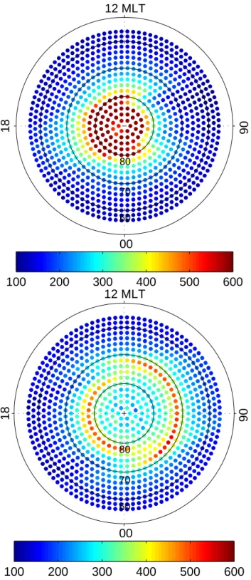
600

Fig. 2. Distribution of sample number per bin for the Northern (top)

and Southern (bottom) Hemisphere. In the north a high sample fre-quency of 600 per bin is attained within the polar cap, reducing to 100 at sub-auroral latitudes. In the Southern Hemisphere the sam-ples are distributed more evenly.

3 Statistical features of polar region winds

For this first CHAMP-based statistical study of high-latitude thermospheric winds we considered the time interval 16 April to 25 August 2003 centred on the June solstice. After binning the readings of the 2053 passes (in each hemisphere) in the way described in the previous section, we obtain indi-vidual maps for both hemispheres. The number of readings per bin is quite large. This helps one to obtain statistically significant results. Figure 2 shows the distribution of sample numbers per bin for the northern and southern polar regions. Within the northern polar cap the bins contain typically 600 samples and at sub-auroral latitudes still more than 100 sam-ples. From a single pass up to three consecutive readings may fall into the same bin. This means that about half of the readings in a bin can be regarded as fully independent sam-ples. Due to the larger offset between the geographic and geomagnetic pole, the sample distribution is different in the Southern Hemisphere. Here, the sample frequency is lower by about a factor of 2 in the polar cap, but at lower latitudes it is more favourable than in the north.

Figure 3 shows the distribution of derived wind speeds in the two hemispheres. In each case the mean velocity calcu-lated for a bin represents an independent result. No smooth-ing between neighboursmooth-ing bins was performed. Nevertheless, we find a smooth velocity distribution across both polar re-gions.

In the Northern (summer) Hemisphere (Fig. 3, top) high velocities, partly exceeding 600 m/s, are observed in the polar cap, in particular on the morning side. Another re-gion of high wind speeds is the auroral/sub-auroral 06:00 to 09:00 MLT sector. The auroral regions from noon to late evening and also past midnight are characterised by low wind velocities ranging around 100 m/s.

In the Southern (winter) Hemisphere (Fig. 3, bottom) the wind speed is significantly lower. There is one exception in the pre-midnight auroral region. These measurements seem to be related to a storm/substorm period. A counterpart to that high-velocity patch is also found in the northern auro-ral region. Geneauro-rally, the wind speed across the polar cap is about two-third of that in the north. Qualitatively, the fea-tures are comparable. Again, the auroral regions from noon to evening and the sector past midnight are dominated by low wind velocities.

So far we have looked only at the distribution of the wind speed. Much more information can be obtained if the direc-tion is known. Figure 4 shows the average wind distribudirec-tion in the polar region of both hemispheres. Velocity vectors are plotted for every second bin. Qualitatively, the wind fields look quite similar in both hemispheres. There are a number of specific features that are more evident in the north. For that reason we will start with that hemisphere.

Poleward of 80◦_{cgm lat. (polar cap) we find the highest}

velocities directed from noon to midnight. On the dawn side we observe strong zonal winds also blowing from day to

18

00

06

12 MLT

100

200

300

400

500

600

06

00

18

12 MLT

100

200

300

400

500

600

Fig. 3. Distribution of the mean thermospheric wind speed (m/s)

in the northern (top) and southern (bottom) polar region around the June 2003 solstice.

night. The wind velocity is markedly reduced in the local time sector before 05:00 MLT. The wind pattern is quite dif-ferent on the dusk side. Here we find moderate zonal winds

18

00

06

12 MLT

CHAMP, 2003, June solstice, NH

v=500 m/s

06

00

18

12 MLT

CHAMP, 2003, June solstice, SH

v=500 m/s

Fig. 4. Distribution of mean thermospheric wind vectors in the

Northern (summer) (top) and Southern (winter) (bottom) Hemi-sphere for June solstice conditions. The vectors are recovered from multiple single component wind measurements.

at sub-auroral latitudes. Along the auroral oval there is a wind stagnation zone reaching from 19:00 MLT until mag-netic noon. Poleward of that zone an anti-cyclonic vortex forms with a focal point near 70◦_{cgm lat. in the 18:00 MLT}

sector. Around midnight the predominant wind direction is duskward.

When looking at the southern polar region, in principle, all the mentioned features can also be recognised. However,

1098 H. L¨uhr et al.: Average thermospheric wind patterns over the polar regions, as observed by CHAMP

18

00

06

12 MLT

0

10

20

30

06

00

18

12 MLT

0

10

20

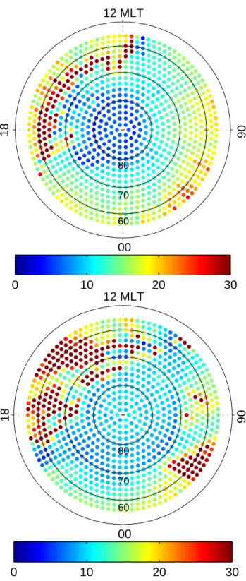
30

Fig. 5. Relative standard deviation of the estimated wind vector

(in %) for each bin in Northern (top) and Southern (bottom) Hemi-sphere. The obtained values do not reflect the uncertainty of the measurements but the variability of the prevailing wind.

the day-to-night wind speeds are markedly lower (∼2/3) and the patterns seem to be less organised. It may be stressed

here that the remarkable similarity of wind patterns in the two hemispheres provides further confidence in our approach of wind estimates.

Furthermore, the applied method of wind vector estima-tion allows for the determinaestima-tion of the mean vector uncer-tainty (cf. Eq. 6). The resulting values reflect the variability of wind readings within a bin. It should not be confused with the precision of the wind measurement. This was esti-mated to be 50 m/s. The relative uncertainty of the presented winds in percent is shown in Fig. 5. In the polar cap and in large parts of the auroral oval, where we have good sam-pling statistics, uncertainties do not exceed 10%. Toward the fringes of the considered region the errors approach 20%. Only in areas of vanishing wind speed does the uncertainty exceed, as expected, the 30% level. The low uncertainty can be regarded as an indication that the derived mean wind vec-tors are suitable for further scientific interpretation.

4 Discussion

We have presented the average thermospheric wind pat-terns at polar regions around the 2003 June solstice. It is the first time that a complete quasi-simultaneous picture of both hemispheres is derived from spacecraft (CHAMP) ac-celerometer measurements. The advantage of interpreting accelerations in terms of winds is that the physically clean method requires no special assumptions. Furthermore, satel-lites with high inclination orbits sample the whole polar re-gion. This gives a high statistical significance for the ob-tained distribution.

A certain limitation of our survey is introduced by the fact that only one horizontal wind component (cross-track) can be determined. This requires very homogenous coverage of the whole polar region, in order to obtain an unbiased mean ve-locity. The CHAMP mission, with its almost 100% data cov-erage and fast precession through all local times, overcomes this problem. For the recovery of the mean wind vector af-filiated to a bin the whole ensemble of measurements falling into that bin is considered, although the individual samples were taken at different times. We regard the implicitly as-sumed condition of stationarity as justified because of the large number of samples in a bin (100–600). This is sup-ported by the relative small uncertainty of the mean values (10%–20%) (cf. Fig. 5).

An advantage of the presented results compared to ground-based observations is the good spatial resolution (220×230 km). Furthermore, seasonal and hemispheric ef-fects can be investigated for identical geophysical conditions. A drawback of the applied method is that it cannot be used for studying transient effects, such as the response of the wind direction to the IMF By. A given pass delivers only

one wind component. From that it is not possible to distin-guish between changes in magnitude or direction.

In the following we will thus focus on the average con-ditions. The year 2003 was characterized by a decline in sun spot number, while the geomagnetic activity reached its peak within this solar cycle. For the period under study we computed the median (average) solar flux index, F10.7=124 (128), and obtained for the magnetic activity, Ap=21 (24)

(corresponding to Kp=4−). Thus, the prevailing conditions

suggest enhanced electrodynamic effects, whereas the hydro-dynamic processes, which depend more on the solar EUV in-tensity, are expected to be reduced. The thermospheric winds are regarded as being influenced by both forces.

When looking at the wind vector plots (Fig. 4) we find strong day-to-night winds over the polar cap. In this re-gion, the pressure gradient force of the neutral density and the mean plasma drift directions are well aligned. It is there-fore no surprise to observe anti-sunward wind speeds of more than 600 m/s in the north. In the Southern (winter) Hemi-sphere peak values are slightly lower. Opposed to the situa-tion at the polar cap, the plasma is generally streaming sun-ward along the auroral oval on the dawn and dusk sides. In those regions there is a competition between neutral and elec-trodynamic forces.

In the Northern (summer) Hemisphere particularly clear wind patterns are derived. Both the strong zonal winds on the dawn side along the auroral oval, and the formation of a clockwise vortex on the dusk side can be explained by the effect of the Coriolis force. Since we are using an Earth-fixed frame for the velocities, this additional force has to be taken into account. Particles starting from noon and mov-ing westward experience a centrifugal force equatorward and the Coriolis force poleward. The polar distance, θ , at which these forces balance, depends on the zonal speed, v, and can be calculated for the size of the Earth and at the CHAMP altitude as

sin θ = v/985, (7)

where v is measured in m/s. For θ =30◦_{we obtain v=498 m/s.}

This value fits well the range of zonal velocities that we ob-serve in the dawn sector. For eastward air flow Coriolis and centrifugal forces both push the particles equatorward. Ac-cording to the scheme presented by Fuller-Rowell and Rees (1984), an eastward zonal wind will be deflected clockwise forming an arc of an anti-cyclonic spiral. The radius of the vortex depends on the initial zonal velocity and on the dis-tance from the pole. This behaviour matches exactly our ob-servations in the dusk sector (cf. Fig. 4, top). Zonal winds near the dusk side polar cap are bent clockwise heading to-wards the equator before they leave our field of view. Faster streams exhibit larger bending radii.

Another obvious feature in both hemispheres is the wind stagnation in the cusp region (cf. Fig. 4). As was shown in earlier studies, this region is characterized by an air up-welling fuelled by Joule heating (L¨uhr et al., 2004; Schlegel et al., 2005). In a dedicated model study Demars and Schunk

(2007) could reproduce the experimental data, and they fur-thermore predict divergent horizontal winds flowing away from the cusp in all directions. When combining their re-sults with the background winds they seem to be in good agreement with our observations.

The effect of the plasma drift on the thermospheric air mo-tion is also quite evident. Along the auroral oval on the dusk side, where the plasma streams sunward, we observe a zone of wind stagnation. In the pre-midnight sector plasma motion bends the cross-polar cap wind duskward, and in the post-midnight sector the counter-streaming plasma and neutrals largely cause wind stagnation. In the dayside sub-auroral re-gions we observe anti-sunward zonal flows on both sides of noon. These may be supported by the sub-auroral plasma drifts (e.g. Foster and Vo, 2002).

When looking at the Southern (winter) Hemisphere we no-tice the clearly weaker cross-polar cap flow. The average speed of all bins between 80◦ _{and 90}◦_{cgm lat. is 490 m/s}

in the north and 300 m/s in the south. This difference can clearly be regarded as a seasonal effect. When assuming sim-ilar plasma drift velocities in both hemispheres, the ion drag, closely controlled by ion/neutral collision frequency, must be lower in the winter hemisphere. This proposition is consis-tent with a lower electron density in the F region of the dark polar cap.

In this context, the seasonal effects on polar cap plasma convection orientation were studied by Jayachandran and MacDougall (1999). They found that plasma is streaming towards midnight in the winter hemisphere and towards pre-midnight hours in summer. This anti-clockwise rotation of the high-latitude electric field pattern by about 21_{/2h during}

winter had been mentioned earlier (e.g. de La Beaujardiere et al., 1991; Ruohoniemi and Greenwald, 1995). Opposed to that, our wind velocity is rotated clockwise by about 15◦_in

the winter hemisphere. We strongly suggest that the observed deflection of the thermospheric wind is caused by the Corio-lis force. An air parcel moving in the anti-sunward direction is continuously deflected in the −uydirection, and the lower

the ux velocity, the stronger the deflection. Consequently,

a clockwise rotation of the 35% slower air flow in the dark hemisphere is expected. For completeness, we also checked the prevailing IMF Byconditions and found an average value

of By=−0.2 nT for the studied period. This value is too small

to account for the observed rotation of wind direction. At lower latitudes we find almost identical wind patterns in the two hemispheres on the night side (18:00–06:00 MLT). Conversely, on the dayside (06:00–18:00 MLT) larger differ-ences are evident. This observation is consistent with the finding of Wang et al. (2005), who reported that seasonal dif-ferences in the auroral current systems are largely confined to the dayside of the oval. The night-side currents are almost unaffected by solar illumination conditions. Highlighting these seasonal differences was the prime reason for choosing the June solstice for this first example of polar region wind pattern derived from CHAMP accelerometer measurements.

1100 H. L¨uhr et al.: Average thermospheric wind patterns over the polar regions, as observed by CHAMP Thermospheric winds at polar latitudes were recorded

ear-lier by the DE-2 satellite. A dedicated study of both hemi-spheres during the 1980/81 and 1981/82 December solstices was conducted by Thayer et al. (1987). Due to sampling limi-tations, not all local times could be covered and only a coarse binning of 5◦_{lat. by 1 h in MLT was used for the estimation}

of mean wind vectors. Their results show some features in agreement with ours, for example, strong day-to-night winds across the polar cap, fast zonal flows on the dawn side and an indication of an anti-cyclonic vortex on the dusk side of the summer hemisphere. However, our results do not con-firm their prominent sunward winds at auroral latitudes on the dusk side. In general, DE-2 shows a rather tight relation between the expected plasma drift and the reported neutral wind. This may partly be due to the solar maximum con-ditions. Based on ground observations of plasma drift and thermospheric wind for the same solar maximum years, Mc-Cormac and Smith (1984) found, however, a much weaker response of the neutral wind to external influences, such as the IMF By, than was observed in the plasma drift.

Consis-tent with these later findings, our average wind distribution also shows less resemblance to the average plasma drift pat-tern.

As mentioned before, there are several forces acting on the neutral particles. Unfortunately, these forces are ordered best in different coordinate systems. The pressure gradi-ent, for example, is sorted best in solar local time and ge-ographic latitude, the Coriolis force in gege-ographic latitude and the plasma motion in magnetic local time and magnetic latitude. For the presentation of the CHAMP-derived winds we used the geomagnetic frame in order to emphasize the in-fluence of electrodynamic forces. In the Northern (summer) Hemisphere this sorting provides rather clear results. In the south the offset between geomagnetic and geographic poles is significantly larger. This influences the balance between ion drag, Coriolis force and curvature term. It is therefore no surprise that the wind pattern in the Southern Hemisphere is so well ordered.

In summary, we have presented the thermospheric wind distribution in the polar region for different solstice condi-tions. Important seasonal differences could be identified, such as the reduction of the day-to-night wind velocity over the polar cap by about 35% in the winter hemisphere. Also the zonal winds at sub-auroral latitudes from noon to dawn and to dusk are significantly reduced under winter condi-tions. Generally, seasonal differences are much more pro-nounced in the dayside auroral zone than on the night side. In addition, we identified hemispheric differences likely caused by the difference in offset of the geomagnetic pole. Investi-gations of further time intervals are required to better distin-guishing between the two prevailing effects.

The technique presented here can only provide an aver-age picture of a 4-month time period. This minimum “expo-sure time” of 131 days is needed to obtain evenly distributed samples at all local times. In this way a fairly independent

picture of the hemispheric differences can be generated for each season. Our approach may therefore be regarded as a suitable tool for climatologically studies. When considering the CHAMP data set, which starts in August 2000 and is ex-pected to continue until middle of 2009, almost a full solar cycle may be covered in a coherent way. This would provide a marvellous benchmark for testing upper atmospheric wind models.

We regard this study as a first step and an appetizer for a better characterization of the high-latitude neutral wind structures. The understanding of the high-latitude neu-tral wind patterns is indispensable for a proper characteri-zation of the magnetosphere-ionosphere-thermosphere cou-pling. The recent CHAMP measurements may help to reach that goal.

Acknowledgements. We thank W. K¨ohler for pre-processing the

Accelerometer data used in this study. The operational support of the CHAMP mission by the German Aerospace Center (DLR) and the financial support for the data processing by the Federal Min-istry of Education and Research (BMBF), as part of the Geotechnol-ogy Programme, are gratefully acknowledged. The DFG supported S. Rentz through the Priority Programme “CAWSES”, SPP 1176.

Topical Editor U.-P. Hoppe thanks two referees for their help in evaluating this paper.

References

Aruliah, A. L., Farmer, A. D., Rees, D., and Brandstrøm, U.: The seasonal behaviour of high-latitude thermospheric winds and ion velocities observed over one solar cycle, J. Geophys. Res., 101, 15 701–15 711, 1996.

Condrescu, M. V., Fuller-Rowell, T. J., Foster, J. C., Holt, J. M., and Cariglia, S. J.: Electric field variability associated with the Millstone Hill electric field model, J. Geophys. Res., 105, 5265– 5273, 2000.

de La Beaujardiere, O., Alacayde, D. A., Fontanari, J., and Leger, C.: Seasonal dependence of high-latitude elelctric fields, J. Geo-phys. Res., 96, 5723–5735, 1991.

Demars, H. G. and Schunk, R. W.: Thermospheric response to ion heating in the dayside cusp, J. Atmos. Solar-Terr. Phys., 69, 649– 660, 2007.

Emmert, J. T., Fejer, B. G., Shepherd, G. G., and Solheim, B. H.: Climatology of middle-and low-latitude daytime F region distur-bance neutral winds measured by Wind Imaging Interferometer (WINDII), J. Geophys. Res., 106, 24 701–24 712, 2001. Forbes, J. M., Roble, R. G., and Marcos, F. A.: Magnetic activity

dependence of high-latitude thermospheric winds and densities below 200 km, J. Geophys. Res., 98, 13 693–13 702, 1993. Foster, J. C. and Vo, H. B.: Average characteristics and activity

dependence of the sub-auroral polarization stream, J. Geophys. Res., 107(A12), 1475, doi:10.1029/2002JA009409, 2002. Fuller-Rowell, T. J. and Rees, D.: Interpretation of an anticipated

long-lived vortex in the lower thermosphere following simulation of an isolated substorm, Plant. Space Sci., 32, 69–86, 1984. Jayachandran, P. T. and MacDougall, J. W.: Seasonal and Byeffect

on the polar cap convection orientation, Geophys. Res. Lett., 26, 975–978, 1999.

Killeen, T. and Roble, R. G.: Thermosphere dynamics: Contribu-tions from the first 5 years of the Dynamics Explorer program, Rev. Geophys., 26, 329–367, 1988.

Killeen, T., Roble, R. G., Smith, R. W., Spencer, N. W., Meriwether, J. W., Rees, D., Hernandez, G., Hays, P. B., Cogger, L. L., Sipler, D. P., Biondi, M. A., and Tepley, C. A.: Mean neutral circulation in the winter polar F-region, J. Geophys. Res., 91, 1633–1649, 1986.

Liu, H., L¨uhr, H., Henize, V., and K¨ohler, W.: Global distribution of the thermospheric total mass density derived from CHAMP, J. Geophys. Res., 110, A04301, doi:10.1029/2004JA010741, 2005. Liu, H., L¨uhr, H., Watanabe, S., K¨ohler, W., Henize, V., and Visser, P.: Zonal wind in the upper thermosphere observed by CHAMP: Climatology, J. Geophys. Res., 111, A07307, doi:10.1029/2005JA011415, 2006.

L¨uhr, H., Rother, M., K¨ohler, W., Ritter, P., and Grunwaldt, L.: Thermospheric up-welling in the cusp region, evidence from CHAMP observations, Geophys. Res. Lett., 31, L06805, doi:10.1029/2003GL019314, 2004.

Marcos, F. A. and Forbes, J. M.: Thermospheric winds from the satellite electrostatic triaxial accelerometer system, J. Geophys. Res., 90, 6543–6552, 1985.

McCormac, F. G. and Smith, R. W.: The influence of the Interplan-etary magnetic field Y component on the ion and neutral motions in the polar thermosphere, Geophys. Res. Lett., 11, 935–938, 1984.

Rees, D., Fuller-Rowell, T., and Smith, R. W.: Measurements of high latitude thermospheric winds by rocket and ground-based techniques and their interpretation using a three-dimensional time-dependent dynamical model, Planet. Space Sci., 28, 919– 932, 1980.

Richmond, A. D.: Ionospheric dynamics using magnetic Apex co-ordinates, J. Geomagn. Geoelectr., 47, 191–212, 1995.

Richmond, A. D., Ridley, E. C., and Roble, R. G.: A thermo-sphere/ionosphere general circulation model with coupled elec-trodynamics, Geophys. Res. Lett., 19, 601–604, 1992.

Roble, R. G., Emery, B. A., Dickinson, R. E., Ridley, E. C., Killeen, T. L., Hays, P. B., Carignan, G. R., and Spencer, N. W.: Thermo-spheric circulation, temperature and compositional structure of the Southern Hemisphere polar cap during October–November, 1981, J. Geophys. Res., 89, 9057–9068, 1984.

Ruohoniemi, J. M. and Greenwald, R. G.: Observations of IMF and seasonal effects in high-latitude convection, Geophys. Res. Lett., 22, 1121–1124, 1995.

Schlegel, K., L¨uhr, H., St.-Maurice, J.-P., Crowley, G., and Hack-ert, C.: Thermospheric density structure over the polar regions observed with CHAMP, Ann. Geophys., 23, 1659–1672, 2005, http://www.ann-geophys.net/23/1659/2005/.

Thayer, J. P., Killeen, T. L., McCormac, F. G., Tschan, C. R., Pon-thieu, J.-J., and Spencer, N. W.: Thermospheric neutral wind sig-natures dependent on the east-west component of the interplan-etary magnetic field for Northern and Southern Hemispheres, as measured from Dynamics Explorer-2, Ann Geophys., 5, 363– 368, 1987.

Wang, H., L¨uhr, H., and Ma, S.-Y.: Solar zenith angle and merging electric field control of field-aligned currents: A statistical study of the southern hemisphere, J. Geophys. Res., 110, A03306, doi:10.1029/2004JA010530, 2005.

Witasse, O., Lilensten, J., Lathuillere, C., and Pibraret, B.: Merid-ional thermospheric neutral wind at high latitude over a full solar cycle, Ann Geophys., 16, 1400–1409, 1998.