HAL Id: hal-00317331
https://hal.archives-ouvertes.fr/hal-00317331
Submitted on 8 Apr 2004
HAL is a multi-disciplinary open access
archive for the deposit and dissemination of
sci-entific research documents, whether they are
pub-lished or not. The documents may come from
teaching and research institutions in France or
abroad, or from public or private research centers.
L’archive ouverte pluridisciplinaire HAL, est
destinée au dépôt et à la diffusion de documents
scientifiques de niveau recherche, publiés ou non,
émanant des établissements d’enseignement et de
recherche français ou étrangers, des laboratoires
publics ou privés.
band, and a comparison with OH(6-2) rotational
temperatures at Davis, Antarctica
F. Phillips, G. B. Burns, W. J. R. French, P. F. B. Williams, A. R. Klekociuk,
R. P. Lowe
To cite this version:
F. Phillips, G. B. Burns, W. J. R. French, P. F. B. Williams, A. R. Klekociuk, et al.. Determining
rota-tional temperatures from the OH(8-3) band, and a comparison with OH(6-2) rotarota-tional temperatures
at Davis, Antarctica. Annales Geophysicae, European Geosciences Union, 2004, 22 (5), pp.1549-1561.
�hal-00317331�
SRef-ID: 1432-0576/ag/2004-22-1549 © European Geosciences Union 2004
Annales
Geophysicae
Determining rotational temperatures from the OH(8-3) band, and a
comparison with OH(6-2) rotational temperatures at Davis,
Antarctica
F. Phillips1, G. B. Burns1, W. J. R. French1, P. F. B. Williams1, A. R. Klekociuk1, and R. P. Lowe2
1Australian Antarctic Division, Kingston 7050, Tasmania, Australia
2Department of Physics and Astronomy, University of Western Ontario, London N6A3K7, Canada
Received: 30 June 2003 – Revised: 11 November 2003 – Accepted: 20 November 2003 – Published: 8 April 2004
Abstract. Rotational temperatures derived from the OH(8–3) band may vary by ∼18 K depending on the choice of transition probabilities. This is of concern when abso-lute temperatures or trends determined in combination with measurements of other hydroxyl bands are important. In this paper, measurements of the OH(8–3) temperature-insensitive Q/P and R/P line intensity ratios are used to select the most appropriate transition probabilities for use with this band. Aurora, airglow and solar and telluric absorption in the OH(8–3) band are also investigated. Water vapour absorp-tion of P1(4), airglow or auroral contamination of P1(2) and
solar absorption in the vicinity of P1(5) are concerns to be
considered when deriving rotational temperatures from this band.
A comparison is made of temperatures derived from OH(6–2) and OH(8–3) spectra collected alternately at Davis (69◦S, 78◦E) in 1990. An average difference of ∼4 K is found, with OH(8–3) temperatures being warmer, but a dif-ference of this magnitude is within the two sigma uncertainty limit of the measurements.
Key words. Atmospheric composition and structure (air-glow and aurora; pressure, density, and temperature)
1 Introduction
Warming of the troposphere due to increases in greenhouse gas concentrations is associated with enhanced cooling in the stratosphere and mesosphere (Berger and Dameris, 1993; Portman et al., 1995; Akmaev and Fomichev, 1998, 2000). Several authors have used rotational temperatures derived from hydroxyl airglow emissions to investigate trends in the upper mesosphere (Golitsyn et al., 1996; Lysenko et al., 1999; Bittner et al., 2002; Burns et al., 2002; Espy and Stegman, 2002). Hydroxyl airglow emissions originate from a layer near 87 km with a mean thickness of 8 km (Baker and Correspondence to: Gary Burns
(gary.burns@aad.gov.au)
Stair, 1988) and can be used as a proxy for kinetic tempera-ture at ∼87 km (She and Lowe, 1998).
Hydroxyl airglow rotational temperatures are derived by comparing intensities of two or more lines from different up-per rotational states, as up-per Eq. (1):
T = (hc/k)(Fb−Fa)/ln[IaAb(2Jb0+1)/IbAa(2Ja0+1)]
. (1)
Fa, Fbare the energy levels of the initial rotational states (the energy level values as given by Coxon and Foster, 1982, are used); Ia, Ibare the emission intensities of the OH lines from different upper states; Aa, Abare the transition probabilities;
Ja0, Jb0 are the upper state, total angular momentum quantum numbers; and h, c and k are Planck’s constant, the speed of light and Boltzmann’s constant, respectively. Transition probabilities are used to apportion the percentage of the up-per rotational states that decay via the transitions measured.
Hydroxyl bands are designated by transitions from an up-per state, v0 (=vibration quantum number), to a lower state, v00, as the OH(v0–v00) band. As 1v increases the bands be-come less intense and appear at lower wavelengths. The choice of band to monitor is thus generally selected based on the upper wavelength limit of the detector. The hydroxyl line nomenclature used in this paper is similar to that pre-sented by Osterbrock and Martel (1992) and Osterbrock et al. (1996, 1997). A summary is presented in the Appendix.
Rotational temperatures have been derived from OH(6–2) spectra collected at Davis Station, Antarctica (69◦S, 78◦E) during 1990 and each winter since 1995 using a Czerny-Turner spectrometer (CTS, Burns et al., 2002). The OH(6–2) band near λ 840 nm is the brightest band that can be mea-sured with GaAs photomultipliers. Greet et al. (1998) ex-amined the minor spectral features, auroral and Fraunhofer contamination of the OH(6–2) P-branch to quantify uncer-tainties for climate studies.
Absolute values of derived hydroxyl rotational temper-atures depend on the transition probabilities, Aa, Ab in Eq. (1). The discrepancy in published transition probabil-ities increases with higher 1v bands, resulting in increas-ing discrepancies in the determined temperatures (Turnbull
and Lowe, 1989; hereafter T&L). For example, Langhoff et al. (1986; hereafter LWR) OH(6–2) transition probabili-ties yield an average winter hydroxyl temperature at Davis of 206 K (Burns et al., 2002) compared with 211 K, if Mies (1974, hereafter Mies) transition probabilities are used and 218 K, if the T&L transition probabilities are used, giving differences of 5 K and 12 K, respectively. In comparison, for an analysis of the OH(8–3) band that returns a tempera-ture of 206 K using the LWR probabilities, the corresponding temperature using the Mies OH(8–3) transition probabilities would be 213 K and 224 K for the T&L transition probabil-ities, giving differences of 7 K and 18 K, respectively. In-tensity ratios of emissions from the same hydroxyl upper state are independent of the kinetic temperature. French et al. (2000) measured these temperature-independent ratios for the OH(6–2) band and compared them with ratios calculated using LWR, Mies and T&L transition probabilities. They found that LWR values were most compatible with the ex-perimental measurements. Pendleton and Taylor (2002) pro-vide a theoretical interpretation of the French et al. (2000) results. When comparing temperatures from different transi-tional bands or with temperatures derived by other methods, particularly bands with high 1v, care must be taken to ensure that the choice of transition probabilities does not introduce an offset in the hydroxyl temperatures.
Differences in hydroxyl rotational temperatures derived from different bands have been interpreted as providing ev-idence for a height variation of hydroxyl upper state vibra-tional levels. This is a possible source of hydroxyl tempera-ture variability when different bands are measured. Theoreti-cal considerations suggest the vertiTheoreti-cal distribution for v0=1 to v0=9 is 1 to 2 km (McDade, 1991). The average winter tem-perature gradient measured at Syowa (69◦S, 39◦E) using a sodium lidar is −1.7 K km−1, at 87 km (Burns et al., 2003). The temperature difference due to variations in average alti-tudes is expected to be small for small 1v0.
The OH(8–3) band was commonly used for hydroxyl tem-perature measurements in past years (for example, Takahashi et al., 1974; Takahashi and Batista, 1981; Myrabo, 1984; Sivjee and Hamwey, 1987). In particular, hydroxyl airglow OH(8–3) band measurements have been made in Antarctica as early as 1979 (Stubbs et al., 1983; Williams, 1996). A de-sire to understand this spectral region, with the possibility of recovering more accurate rotational temperatures from early records, prompted this research.
In 1990 at Davis Station, Antarctica, spectra were col-lected alternately in the OH(8–3) and (6–2) region. In 1999, high-spectral-resolution, full-band OH(8–3) spectra were collected over a 5 week period. In this paper, these high-resolution spectra are used to identify possible auroral and Fraunhofer contamination, and the location of spectral features which may effect temperature determinations from the OH(8–3). Temperature-independent intensity ratios are determined from the high-resolution spectra and compared with the ratios predicted by published transition probabili-ties to determine which transition probabiliprobabili-ties are most ap-propriate to use when determining rotational temperatures
in this band. Information gained from the high-resolution 1999 spectra is used to determine rotational temperatures from OH(8–3) spectra collected in 1990. These temperatures are compared with temperatures from alternately collected OH(6–2) spectra, derived using information on this band published by Greet et al. (1998) and French et al. (2000), to quantify differences which may influence temperature trends determined from combining measurements of these bands from different eras.
2 Instrumentation and data
Spectra were collected with a scanning Czerny-Turner spec-trometer (CTS) at Davis during 1990 and 1999, using a cooled (−28◦C) GaAs photomultiplier. The CTS has a 6◦ field-of-view (fov). An expanded description of the in-strument is provided by Williams (1996).
Spectral response is determined by scanning a low bright-ness source (LBS) which uniformly illuminates the instru-ment’s fov. The lamp is calibrated against a spectral stan-dard at the Australian Measurement Laboratories. A total of 63 scans from four separate occasions were collected dur-ing 1999. The LBS intensities at λ724 nm and λ740 nm, the largest separation of lines compared, yielded a consistent cal-ibration ratio to within 0.4%.
In April 1999, the CTS was aligned to the zenith and scanned OH(8–3) R-, Q-, and P-branches from λ723.5 to λ740.5 nm at intervals of 0.005 nm and an integration time of 0.5 s. Acquisition time for each spectrum was 32 min. An order-separating filter (λ<475 nm) limited observations to the first order. Rowland “ghosts” (Longhurst, 1957) of magnitudes 0.5% and 0.2%, displaced by 0.3 nm and 0.6 nm, respectively, were measured. An instrument profile of 0.086 nm full-width-at-half-maximum (fwhm) was deter-mined for these measurements. Knowledge of the instrument function is needed to allow for contamination by lines not fully resolved from adjacent features. This is important for the determination of intensity ratios of emissions from the same upper state. A frequency stabilised laser was used to define the instrument function at 632.82 nm. Two equal in-tensity functions of the measured laser profile separated by the OH(8–3) P1(3) 3-doublet spacing (0.0145 nm) are then
best-fitted to an average P1(3) profile by jointly varying the
fwhm of the two laser profiles. The fwhm-adjusted laser profile is the instrument function at the P1(3) wavelength,
λ734.1 nm.
During 1990, the optical axis of the CTS was aligned 30◦ above the SE horizon (azimuth 130◦E), away from the most aurorally active region of the sky. Spectra were accumula-tions of five sequential scans, with photon counts in each scan made at 0.1-s integration and 0.005-nm intervals. OH(8–3) and (6–2) P-branch spectra were acquired alternately. For the OH(8–3) band, each spectrum covers λ730 to λ744.5 nm and took ∼50 min to acquire. For the OH(6–2) band, each spectrum covers λ837.5 to λ856.0 nm and took an hour to acquire. The instrument function at OH(8–3) wavelengths
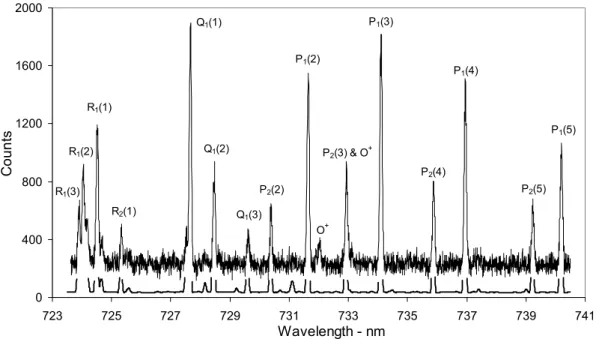
P1(3) P1(2) P1(4) P1(5) Q1(1) Q1(2) R1(1) R1(2) R1(3) R2(1) Q1(3) P2(2) O+ P2(3) & O+ P2(4) P2(5) 0 400 800 1200 1600 2000 723 725 727 729 731 733 735 737 739 741 Wavelength - nm Cou nt s
Fig. 1. OH(8–3) hydroxyl airglow (94 summed spectra, clear skies or “thin cloud”, Moon below horizon, no aurora apparent). A theoretical
spectrum, plotted below the summed spectrum, indicates the expected thermalized hydroxyl airglow contribution to the background.
has a fwhm of ∼0.158 nm and at OH(6–2) wavelengths has a fwhm of ∼0.154 nm.
In 1990, a calibration lamp was scanned on 9 separate oc-casions, with 5 scans on each occasion. The lamp was first calibrated against a spectral standard in 1996. It has been as-sumed that the 1996 calibration measures the spectral shape in 1990 (see Greet et al., 1998). Spectral calibration uncer-tainties for the 1990 spectra equate to a 2.0 K uncertainty in derived temperatures from both the OH(8–3) and OH(6–2) bands.
The CTS was operated without an appropriate order sep-aration filter during 1990. This does not significantly ef-fect the OH(8–3) spectra, but results in the dominant auroral contamination in the 1990 OH(6–2) spectra being second-order N+21Neg (0–1) and (1–2) band emissions. Further de-tails of the 1990 OH(6–2) spectra are presented by Greet et al. (1998), but we adopt a different approach to background removal which is noted later.
A broad classification of sky conditions (clear, thin cloud, patchy cloud, overcast) was maintained through visual obser-vation and (1999 only) reference to an all-sky video system. The “thin cloud” classification describes times of uniform, thin, high cloud, through which bright stars are visible. Dur-ing cold Antarctic winters at Davis, this is a common sky condition.
When selection against auroral contamination was re-quired, reference was made to wide-angle (60◦fov), zenith-oriented photometer measurements of the aurorally activated N+21NG band at λ428 nm.
Data acquired during twice-daily balloon flights con-ducted by the Australian Bureau of Meteorology at Davis were used to determine atmospheric water vapour content.
3 The OH(8–3) spectral region and its contamination The dominant emissions of the OH(8–3) spectral region are labelled in Fig. 1. The spectrum in Fig. 1 is a summation of 94 of the April 1999 spectra for which the sky conditions were classified as clear or “thin cloud” (hereafter referred to as “clear sky”) and no auroral emission was apparent in the wide-angle photometer monitoring the N+21NG (0–1) band at λ428 nm. The broad features of the R-, Q- and lower rota-tional state P-branch structure are apparent.
A theoretical hydroxyl spectrum derived from LWR tran-sition probabilities using a temperature of 214 K, convolved with our instrument function (including the grating Rowland ghosts which are just visible for the most intense lines at the resolution displayed), is presented below at the combined spectrum in Fig. 1. It shows minor OH features at the mag-nitude they are expected within the background. The tem-perature used to derive the theoretical spectrum is the “best-fit” value determined from the summed spectrum. Tables 1 and 2 include lists of the wavelengths of the major OH(8– 3) lines and weak intensity hydroxyl features in this spectral region, respectively. Adjacent spectral emissions contribute to the intensities at specified wavelengths depending on the instrument function. The wavelength location of the maxi-mum intensity may also be slightly shifted in this manner. To provide the reader with an indication of the relative inten-sities of significant OH(8–3) emissions, also listed in Table 1 are the expected and measured peak intensities and locations of the major features relative to P1(3). The relative
theoret-ical peak intensities and locations are determined after con-volution with the instrument function. Note that the spec-trum compared is the sum of 94 individual spectra of vary-ing temperatures, and these comparisons thus serve only as a
Table 1. The main OH(8–3) branch lines. A theoretical spectrum
(LWR, 214 K) has been convolved with the instrument function and
the peak wavelength (λpeak conv.) and peak intensity (Ptheory)
rela-tive to the P1(3) emission is listed and compared with measurements
from Fig. 1 (λobsand Pobs). Blended lines are indicated by symbols
(∗, +, x).
Line Oair
(nm) O(nm)peak conv. (nm)Oobs P(%) Theory P(%) obs
R1(3)f e 723.88723.88 723.88 723.89 26.3 25.4 R1(2)f 724.02 e 724.02 724.02 724.03 43.4 42.5 R1(4)e 724.09 * f 724.09 * R2(3)e 724.14 * f 724.15 * R2(4)e 724.19 * f 724.20 * 724.12 724.13 19.2 19.2 R1(1)f 724.49 + e 724.49 + R2(2)e 724.51 + f 724.51 + 724.50 724.51 59.1 58.0 R1(5)e 724.65 × f 724.66 × R2(5)e 724.66 × f 724.66 × 724.66 724.66 7.6 12.1 R2(1)f 725.31 e 725.32 725.32 725.32 16.5 16.2 Q2(1)e 727.51 f 727.52 727.51 727.52 12.5 16.2 Q1(1)e 727.64 f 727.64 727.64 727.65 106.1 102.1 Q1(2)e 728.44 f 728.45 728.45 728.46 43.1 39.4 Q1(3)e 729.58 f 729.61 729.59 729.61 16.6 14.1 P2(2)e 730.37 f 730.38 730.38 730.38 25.2 24.9 P1(2)e 731.62 f 731.63 731.63 731.63 80.6 83.1 P2(3)e 732.91 f 732.92 732.92 39.9 P1(3) 734.08 f 734.10 734.09 734.09 100.0 100.0 P2(4)e 735.87 f 735.87 735.87 735.87 36.7 36.1 P1(4)e 736.93 f 736.95 736.94 736.95 82.2 75.2 P2(5)f 739.22 e 739.22 739.22 739.22 26.2 27.0 P1(5)e 740.17 f 740.20 740.19 740.19 49.2 50.6
guide. Goldman (1982) derives satellite line (see Appendix) transition probabilities consistent with Mies transition prob-abilities of the main branch transitions. In order to estimate the satellite line intensities equivalently for LWR transition probabilities, we have scaled the Goldman (1982) values in the same ratio to the appropriate P-branch transition
proba-Table 2. OH(8–3) background features and unthermalised OH emissions. A theoretical spectrum (LWR, 214 K) has been con-volved with the instrument function and the peak wavelength (λpeak conv.) and peak intensity (Ptheory) relative to the P1(3) emis-sion is listed for the thermalised components. Blended lines are indicated by a symbol (∗).
Line
O
air(nm)
O
(nm)
peak conv.P
(%)
TheoryR
2(6)e
725.53 *
f
725.53 *
R
1(6)e
725.58 *
f
725.60 *
725.58
1.8
Q
2(2)e
728.15
728.16
4.2
f
728.17
(7-2) P
2(12)f
728.57
729.22
1.8
e 728.65
(7-2) P
1(12)e
728.97
f 729.11
Q
2(3)e
729.21
f
729.23
Q
2(4)e
730.69
730.69
1.0
f
730.70
Q
1(4)e
731.08
731.11
5.1
f
731.13
QR
12(1)e
734.49
734.49
1.1
f
734.49
(7-2) P
2(13)f
734.69
e 734.79
(7-2) P
1(13)e
735.06
f 735.21
PQ
12(2)e
737.40
737.41
1.4
f
737.41
PQ
12(3)e
739.00
739.01
1.4
f
739.02
bility. These are used to calculate the satellite line theoretical values provided, along with those for other weak-intensity, thermalised hydroxyl emissions in Table 2.
At some level of J0, the hydroxyl rotation state populations become non-thermal (see, e.g. Pendleton et al., 1993). States of high J0may have wavelengths sufficiently different from the dominant band lines, to extend into another band. Mea-sured intensities, while low relative to the major P-branch lines (at most a few %), may be several orders of magnitude larger than the theoretical thermalised intensities (Pendleton et al., 1993). While of low intensity, these emissions may contaminate major lines or background regions in a system-atic manner. Greet et al. (1998) noted and demonstrated that unthermalised OH(5–1) P1(12) emissions are blended with
OH(6–2) P1(3), rendering this major line suspect for
rota-tional temperature determinations. Osterbrock et al. (1996) using spectra from the high resolution (∼0.02 nm) echelle
P1(3) P1(2) P1(4) P1(5) Q1(1) Q1(2) R1(1) R1(2) R1(3) R2(1) & O Q1(3) P2(2) O+ P2(3) & O+ P2(4) P2(5)
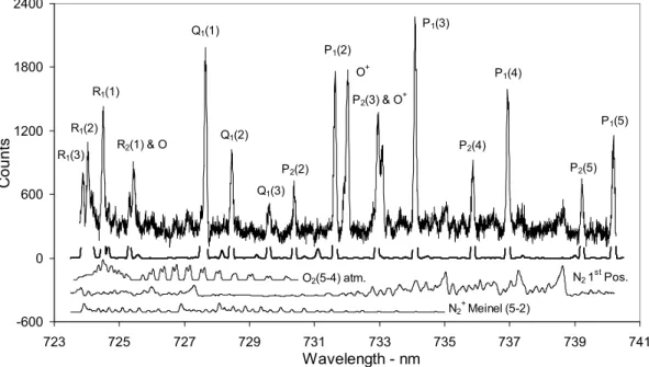
O2(5-4) atm. N21st Pos. N2+Meinel (5-2) -600 0 600 1200 1800 2400 723 725 727 729731 733 735 737 739741 Wavelength - nm C ount s
Fig. 2. Auroral contamination (116 summed spectra, Moon below horizon, aurora apparent). A theoretical hydroxyl and O2(5–4)
Atmo-spheric, N21stPositive and N+2 Meinel (5–2) theoretical auroral spectra are shown below the summed spectrum.
spectrograph on the Keck 10-metre telescope at Mauna Kea, lists the unthermalised OH emissions that extend into the OH(8–3) spectral region. The wavelength of these OH(7–2) emissions are also listed in Table 2. On the long wavelength side of Q1(2) in Fig. 1 is an unassigned feature that could be
mistaken for unthermalised OH(7–2) P2(12). We consider
this association unlikely, because OH(7–2) P1(12), which
should be of similar intensity, is not as readily apparent in the spectrum. We can make no definitive assignment for the feature noted.
Despite our efforts, some high-altitude dayglow or weak auroral features are apparent in Fig. 1. The O+(2Po1/2→2Do5/2)emission at λ731.92 nm and the more
intense O+(2Po3/2→2Do5/2) emission at λ732.02 nm are
merged at our instrument resolution but separated from P1(2) at λ731.63 nm. Values derived from our spectra
are used for these wavelengths (see later in this section), but the “air” wavelengths listed in the Atomic Line List (www.pa.uky.edu/∼peter/atomic/) are used for other atomic and ionic emissions. Further O+ emissions at λ732.97 nm (2Po1/2→2Do3/2)and at λ733.07 nm (2Po3/2→2Do3/2)are
blended with P2(3) at λ732.92 nm. These O+ lines result
from a metastable state with a theoretical radiative lifetime of ∼5 s (Smith et al., 1982). The upper state is activated by low energy auroral electrons or sunlight. Collisional deacti-vation limits intense O+emissions at λ732 nm and λ733 nm to altitudes above 200 km (Rusch et al., 1977; Smith et al., 1982). The high altitude of these ionic emissions means they can still be activated by sunlight after the hydroxyl layer at ∼87 km is in darkness. For this reason, specific care must be taken when deriving rotational temperatures using low-resolution (fwhm>∼0.16 nm) measurements of the OH(8–3) P1(2) line which may be contaminated by dayglow O+
emis-sions collected when the Sun is illuminating the atmosphere at ∼300 km (solar elevation >−17◦for zenith observations). N21stPositive (6–4), (5–3), (4–2), N+2 Meinel (5–2) and
O2(b16g+−X36g)(5–4) bands potentially contaminate the
OH(8–3) band. Figure 2 is a summation of 116 spectra collected when optical aurora is apparent on the wide-angle photometer monitoring the N+2 1NG (0–1) band at λ428 nm and the Moon is below the horizon. The O+emissions near
λ732 nm and those blended with P2(3) near λ733 nm are
sig-nificantly more intense relative to the OH features in Fig. 2 than in Fig. 1, indicating an auroral contribution to their in-tensity. An atomic oxygen triplet near λ725.44 nm, from the transitions3So1→3P0,1,2, is also readily apparent. The
in-tensity of the atomic and ionic auroral emissions in Fig. 2, relative to the OH(8–3) P1(3) intensity, are listed in Table 3.
To assist with the determination of auroral band features in this spectral region, theoretical spectra of the O2(5–4)
atmo-spheric, the N+2 Meinel (5–2) and the summed N21stPositive
bands [(5–3), (6–4) and (4–2)] have been convolved with the instrument function and separately displayed below the com-bined, measured spectra in Fig. 2. The N21stPositive (3–1)
and (7–5) and N+2 Meinel (6–3) bands do not extend into the OH(8–3) spectral range considered, and the N+2 Meinel (4–1) band contributes less than 3% of the auroral contami-nation at any wavelength in the OH(8–3) spectral range con-sidered. Programs for generating synthetic auroral spectra of the nitrogen bands were obtained by private communication (Gattinger; see also Gattinger and Vallance Jones, 1974). A temperature of 300 K is used for the theoretical nitrogen au-rora spectra.
The N21st Positive (5–3) band is the dominant auroral
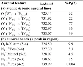
P1(3) P1(2) P1(4) P1(5) Q1(1) Q1(2) R1(1) R1(2) R1(3) R2(1) Q1(3) P2(2) O+ P2(3) & O+ P2(4) P2(5) telluric solar + telluric solar -800 0 800 1600 2400 3200 4000 4800 5600 723 725 727 729 731 733 735 737 739 741 Wavelength - nm Co un ts
Fig. 3. Scattered moonlight influence (126 summed spectra, scattered moonlight, no aurora apparent). The Kitt Peak solar and telluric
spectra, both combined and separately, and a theoretical hydroxyl spectrum are shown below the summed spectrum.
Table 3. Airglow and auroral, atomic and ionic lines and molecular
bands in the OH(8–3) region, their wavelength of peak intensity within the interval λ723 nm to λ741 nm and their intensity relative
to OH(8–3) P1(3) (scaled from Fig. 2).
Auroral feature Oair(nm) %P1(3)
(a) atomic & ionic auroral lines
O (3So1o3P0,1,2) 725.44 32 O+ (2Po1/2o2Do5/2) 731.92 22 O+ (2Po3/2o2Do5/2) 732.02 77 O+ (2Po 1/2o2Do3/2) 732.97 36 O+ (2Po 3/2o2Do3/2) 733.07 39
(b) auroral bands (O peak in region)
O2 b-X Atm (5-4) 724.50 9.9
N2 1stPos (6-4) 727.30 5.3
N2+ Meinel (5-2) 728.07 4.5
N2 1st Pos (5-3) 738.63 15
N2 1st Pos (4-2) 739.99 0.004
N21stPositive theoretical spectrum has been matched to the
combined, measured spectra by minimising the least-square residuals to selected portions within this region of the spec-trum. This “best-fit” theoretical spectrum is used to set the intensity for theoretical calculations of all nitrogen aurora in this region, including the N+2 Meinel (5–2) band. The peak intensities and associated wavelength of each of the auroral N21stPositive bands and the N+2 Meinel (5–2) band in Fig. 2,
as determined from the theoretical spectra, are listed in Ta-ble 3. These values, which are listed relative to the peak P1(3)
intensity, depend on the intensity of the aurora but provide an indication of the relative importance of the auroral bands in the OH(8–3) spectral region for average auroral conditions at Davis (magnetic latitude 74.6◦S). When viewing Table 3, please note that the N21stPositive (4–2) band is more intense
at longer wavelengths than within the OH (8–3) spectral re-gion considered.
The O2 b-X Atmospheric (5–4) band is the most
signif-icant auroral band contaminant in the R- and Q-branch re-gions, although the N21st Positive (6–4) and N+2 Meinel
(5–2) bands also contribute. Slanger et al. (1997) have re-ported detection of O2Atmospheric (5–4) nightglow using
the Keck/HIRES spectra from Mauna Kea. The peak in-tensities of the O2b-X Atmospheric (5–4) nightglow lines
are more than two orders of magnitude less intense than the brightest OH(8–3) emissions (Slanger et al., 2000) but can be significantly enhanced during aurora (Gattinger and Vallance Jones, 1976). We have used the theoretical spectrum of the O2b-X Atmospheric (5–4) band published by Slanger and
Osterbrock (1998), convolved with our instrument function, and minimised the least-square residuals of fitting it to a re-gion between the R-and Q-branches. The theoretically deter-mined N21stPositive (6–4) and N+2 Meinel (6–2) band
con-tributions were subtracted before the O2 b-X Atmospheric
(5–4) contribution was determined. Measured in this man-ner, the peak intensity of the O2b-X Atmospheric (5–4) band
relative to the P1(3) emission is ∼10% (see Table 3), strongly
indicating auroral enhancement of this band.
The “air” wavelengths listed in the Atomic Line List for O+(2Po3/2→2Do5/2) and O+(2Po1/2→2Do5/2) are
λ732.00 nm and λ731.89 nm, respectively. A least-squares best-fit of the CTS instrument function to this region of Fig. 2 yields wavelengths of λ732.02 nm and λ731.915 nm
and a relative intensity of 1:0.28. Smith et al. (1982), who observed this region with a Fabry-Perot spectrometer, use a wavelength of λ732.02 nm for the O+(2Po
3/2→2Do5/2)
emission. This value is consistent with our measurement. However, Smith et al. (1982) list in their Abstract a separa-tion of 0.08 nm for these O+lines. This may not be a value that they have measured, and it is not supported by our mea-surements, which indicate a separation of 0.105 ±0.005 nm. Scattered sunlight may influence spectra collected at low solar depression angles or when moonlight and cloud are present. The spectrum in Fig. 3 is a summation of 126 spectra collected when scattered moonlight could enter the field-of-view of the instrument and no auroral activity is apparent. Below this are presented, both combined and separately, so-lar and telluric spectra determined from Kitt Peak spectra at varying solar zenith angles (Wallace et al., 1998), convolved with the CTS instrument function. Both solar and atmo-spheric absorption lines are clearly visible in the CTS spec-trum, and collectively account for the absorption features in the spectrum. Comparison with HITRAN data (Rothman et al, 1998, 2003; www.HITRAN.com) indicates water vapour is the only significant atmospheric absorber in this wave-length region.
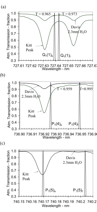
Figures 4a, b and c show expanded portions of the com-bined solar and telluric, high-resolution Kitt Peak spectrum in the vicinity of the Q1(1), P1(4) and P1(5) emissions and
the Doppler-broadened, lamda-doubled, OH emission lines (after Espy and Hammond, 1995). The average winter wa-ter vapour content above Davis in 1999, derived from twice-daily meteorological balloon flights, is 2.3 mm (7.695 E+22 molecules cm−2). Also shown in Figs. 4 a, b and c, are
the pressure-broadened, absorption profiles for typical Davis winter conditions, based on HITRAN 2001 line parameters. For average Davis winter conditions, we calculate that 3.1% of OH(8–3) Q1(1) and 2.3% of OH(8–3) P1(4) are absorbed.
Other OH(8–3) lines of interest with measurable absorption are R1(2) and R1(1). These are, respectively, 1.2% and 0.6%
absorbed. A table of atmospheric absorption of the major OH(8–3) lines for a range of atmospheric conditions printed in Espy and Hammond (1995) is unfortunately a printing er-ror, being a repeat of the OH(6–2) Table. The actual values calculated for that paper are comparable with our estimates (Espy, private communication). The absorption by water vapour for the lines noted will be significantly exacerbated at lower latitude sites, which typically have much wetter at-mospheres. Espy and Hammond (1995) use 29, 21, 8.5 and 4.2 mm of H2O as typical mid-latitude summer, high-latitude
summer, mid-latitude winter and high-latitude winter atmo-spheric water vapour content estimates.
Typically P-branch hydroxyl lines are used to derive ro-tational temperatures. In order to quantify the effect of at-mospheric water vapour on temperatures derived using the OH(8–3) P1(4) emission, consider a relatively dry
atmo-sphere containing 5 mm of water vapour. Zenith measure-ments of the P1(4) intensity would be reduced by ∼5%
and temperatures derived using LWR transition probabili-ties from the P1(2)/P1(4) intensity ratio would be reduced
(a)
(b)
(c)
0.3 0.4 0.5 0.6 0.7 0.8 0.9 1.0 740.15 740.16 740.17 740.18 740.19 740.2 740.21 Wavelength - nm Atm. Tran smis sion - fraction Davis 2.3mm H2O Kitt Peak P1(5)f P1(5)e 0.3 0.4 0.5 0.6 0.7 0.8 0.9 1.0 736.90 736.91 736.92 736.93 736.94 736.95 736.96 Wavelength - nm Atm. Tran smission - fra ctio n Davis 2.3mm H2O Kitt Peak T = 0.959 T=0.995 P1(4)e P1(4)f 0.3 0.4 0.5 0.6 0.7 0.8 0.9 1.0 727.61 727.62 727.63 727.64 727.65 727.66 727.67 Wavelength - nmAtm. Transmission - fraction
Davis 2.3mm H2O Kitt Peak T = 0.965 T = 0.973 Q1(1)e Q1(1)f
Fig. 4. An expansion of the OH(8–3) Q1(1), P1(4) and P1(5) spec-tral regions, showing the Kitt Peak combined solar and telluric, high-resolution spectrum and a pressure-broadened, water vapour
spectrum for typical Davis winter conditions (2.3 mm H2O,
HI-TRAN 2001 line parameters). The hydroxyl line e and f compo-nents are shown with appropriate Doppler broadening (after Espy and Hammond, 1995).
by ∼10 K, from the P1(3)/P1(4) ratio would be reduced by
∼17 K and from the P1(4)/P1(5) ratio would be increased by
∼15 K. The magnitude of these errors is dependent on the highly variable atmospheric water vapour content.
Osterbrock et al. (1997) briefly address the issue of atmo-spheric absorption of the hydroxyl airglow lines observed by the Keck telescope on Mauna Kea (altitude ∼4200 m).
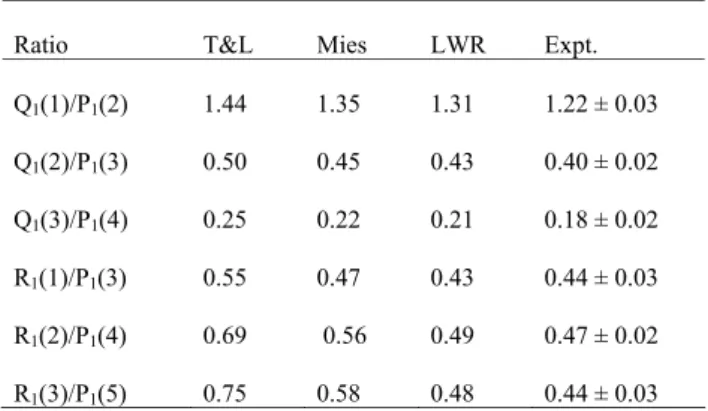
Table 4. OH(8–3) temperature-insensitive intensity ratios derived
from T&L, Mies and LWR transition probabilities and values deter-mined from the summed high-resolution spectrum in Fig. 1.
Ratio T&L Mies LWR Expt. Q1(1)/P1(2) 1.44 1.35 1.31 1.22 ± 0.03 Q1(2)/P1(3) 0.50 0.45 0.43 0.40 ± 0.02 Q1(3)/P1(4) 0.25 0.22 0.21 0.18 ± 0.02 R1(1)/P1(3) 0.55 0.47 0.43 0.44 ± 0.03 R1(2)/P1(4) 0.69 0.56 0.49 0.47 ± 0.02 R1(3)/P1(5) 0.75 0.58 0.48 0.44 ± 0.03
They discuss the OH(8–3) P1(4)e line and its proximity to
a water vapour absorption line, but conclude that absorp-tion did not appear to be significant. The pressure broad-ening of the water vapour lines is significantly less at the altitude of Mauna Kea (∼0.006 nm) compared to sea-level (∼0.008 nm), thus absorption may be significantly reduced for the Mauna Kea site compared with Davis. On-going research utilizing Mauna Kea observations (Cosby, private communication ) supports the possibility of measurable at-mospheric absorption of the OH(8–3) P1(4) emission even
for this high-altitude observatory.
Figure 4c shows an expansion of the P1(5) wavelength
re-gion. P1(5) lies close to a solar absorption line. If scattered
moonlight enters an instrument’s field-of-view, this solar line can potentially be a source of error in determining the inten-sity of P1(5), thus influencing derived temperatures.
4 Temperature-insensitive OH(8–3) intensity ratios Hydroxyl emissions from the same upper rotation-vibration state maintain the same intensity ratio independent of tem-perature. Temperature-independent intensity ratios are deter-mined from the high-resolution summed spectrum in Fig. 1. The 94 spectra contributing to Fig. 1 were collected when the Moon was below the horizon and auroral contamination was negligible. The analysis is similar to that presented by French et al. (2000) for the OH(6–2) region. Photon counts are determined in wavelength regions, centred on emissions of interest. The width of the “count-region” for P1(2), P1(3),
P1(4), Q1(1), Q1(2), R1(1) and R1(3) is 0.155 nm. A
count-region of 0.135 nm is used for P1(5), Q1(3) and R1(2). The
percentage of the emission of interest contained in the count region, and from “blended” emissions, is determined by ref-erence to the instrument function.
For the spectra contributing to Fig. 1, the average wa-ter vapour content dewa-termined from the balloon flights on those days was 1.7 mm. The HITRAN 2001 line parame-ters were used to calculate and to allow for the absorption by this amount of water vapour on the measured OH(8–3)
Q1(1), P1(4), R1(1) and R1(2) intensities. The
contribu-tion of unresolved hydroxyl emissions to the count region is calculated from the instrument function and LWR transmis-sion probabilities at a temperature of 214 K. Error estimates of these contaminations are calculated as the difference ob-tained using LWR transition probabilities at temperatures of 200 K and 230 K. A total uncertainty for each intensity mea-surement is determined by adding in quadrature errors from counting statistics, in estimating the background level, and uncertainties in calculating the contribution of contaminat-ing emissions. The most difficult line intensities to estimate are R1(1), R1(2) and R1(3). R1(1) is significantly blended
with R2(2), with minor contributions from R1(5) and R2(5).
28.2% of the signal under the R1(1) count region is
con-tributed by other hydroxyl emissions. R1(2) is significantly
blended with R1(4), which is itself significantly absorbed by
water vapour (20.0% for 1.7 mm H2O), with minor
contribu-tions from R2(3) and R1(3). 13.0% of the signal under the
R1(2) count region is contributed by other hydroxyl
emis-sions. The R1(3) count region is contaminated by R1(2),
which contributes 6.0% of the measured signal. The count regions for other emissions contain less than a 1% contribu-tion from blended hydroxyl emissions.
The OH(8–3) temperature-insensitive intensity ratios de-termined from the summed 1999 spectrum, along with the corresponding values from Mies, T&L and LWR, are de-tailed in Table 4. The experimentally determined Q/P ratios are lower than the values determined from the published tran-sition probabilities, although the LWR ratios are closest. Of the LWR Q/P ratios, only Q1(1)/P1(2) is significantly
differ-ent from the measured values, being higher by ∼7%. The experimental R/P ratios are significantly lower than the T&L and Mies values but within the measurement uncertainty of the LWR values. The LWR transition probabilities are thus most consistent with temperature-insensitive intensity ratios measured for the OH(8–3) band. French et al. (2000) re-ported that LWR transition probabilities were most consis-tent with the temperature-insensitive intensity ratios in the OH(6–2) band. Therefore, it is appropriate to use LWR tran-sition probabilities when comparing OH(8–3) and OH(6–2) hydroxyl rotational temperatures. No implication can be drawn from our experimental measurements of the relative merit of the absolute values of the published transition proba-bilities, or of the accuracy of the relative differences between vibrational bands (see, for example, Melo et al., 1997).
5 Comparison of OH(6–2) and OH(8–3) winter temper-atures
Rotational temperatures were determined from OH(6–2) and (8–3) spectra collected in 1990, using LWR transition prob-abilities. The intensities of the P1(2), P1(3), P1(4) and P1(5)
emissions were calculated from 0.255-nm wide count regions centred on each emission, with an allowance made for the instrument function and lambda doubling of the lines (as per Greet et al., 1998). Background regions were chosen
160
185
210
235
260
50
100
150
200
250
300
Te
mp
erat
ur
e
(K
)
OH(6-2) T160
185
210
235
260
50
100
150
200
250
300
Te
mp
erat
ur
e
(K
)
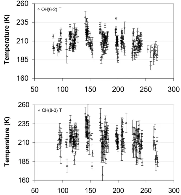
OH(8-3) TFig. 5. OH(6–2) and OH(8–3) rotational temperatures determined from spectra collected at Davis in 1990, with ± one sigma errors.
individually for each emission to match minor auroral and scattered moonlight contaminations, for the instrument func-tion used. Temperatures were calculated for each possible ratio. For the OH(6–2) band, a weighted mean tempera-ture is determined after neglecting those ratios involving the P1(3) emission as this line is blended with the unthermalised
OH(5–1) P1(12) emission (Greet et al., 1998). For the OH(8–
3) band, a weighted mean temperature was determined after ignoring those ratios involving the P1(4) emission. As has
been demonstrated in this paper, measured OH(8–3) P1(4)
intensities vary depending on the atmospheric water vapour content. Figure 5 shows the measured OH(6–2) and OH(8– 3) temperatures and associated one-sigma errors. Average errors for individual spectra are 4 K and 6 K for OH(6–2) and (8–3), respectively. The OH(8–3) errors are generally larger because of the lower intensity of this emission.
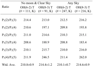
Table 5 shows a comparison of OH(8–3) and (6–2) average temperatures for the winter interval (106≤day-of-year≤258; Burns et al., 2002) for “any sky” and “no Moon and clear sky” conditions. Standard errors are listed for the weighted-average temperatures. In 1990, spectra were collected in the two-week intervals centred on “new Moon”. Only ∼20% of the “any sky” data are collected with the Moon above the horizon. Excluding these data varies the weighted-average temperatures by no more than 0.4 K. More OH(6–2) spectra were available for analysis, and this is noted in Table 5. This may result in a bias, so a separate comparison using only the temperatures from alternate spectra was made. There are 80 alternate OH(6–2) and OH(8–3) temperature measure-ments from “no Moon and clear” spectra. The average tem-perature difference is 2.6 K and the standard error is 1.2 K, with OH(8–3) temperatures being warmer. For “any sky”
Table 5. Average hydroxyl rotational temperatures for individual
line ratios in the OH(8–3) and OH(6–2) bands over the 1990 win-ter (106≤day-of-year≤258), separately presented for “no Moon and clear sky” and “any sky” conditions. Standard errors are listed for the “weighted average” temperatures.
No moon & Clear Sky Any Sky Ratio OH(6-2) T (# = 111, K) OH(8-3) T (# = 91, K) OH(6-2) T (# = 247, K) OH(8-3) T (# = 216, K) P1(2)/P1(3) 214.4 213.0 212.5 216.2 P1(2)/P1(4) 210.6 197.1 209.8193.8 P1(2)/P1(5) 211.0 214.6 210.3 215.1 P1(3)/P1(4) 208.6 188.9 208.8 183.4 P1(3)/P1(5) 210.1 215.7 210.0 216.0 P1(4)/P1(5) 211.9 246.5 211.4 262.0 Wtd. Ave. 210.8±0.9 214.4±1.2 210.1±0.7 214.6±0.9
conditions, there are 227 alternate spectra measurements. For these, the mean difference is 3.9 K and the standard error is 0.8 K, with the OH(8–3) temperatures again being warmer. After including the results from Table 5, the average temper-ature differences range from 2.6 K to 4.5 K. All are signifi-cant at twice the standard error, however, there are sufficient sources of systematic error that could account for differences of these magnitudes. Combining the spectral calibration er-rors for each band in 1990 in quadrature yields a relative tem-perature uncertainty of 2.8 K. The measured differences are all within twice this uncertainty.
The influence of water vapour absorption on the OH(8–3) P1(4) line ratio temperatures is readily apparent in Table 5.
The result is similar for temperatures determined from the 1999 clear-sky, summed spectrum. To determine the impact of absorption on the P1(4) emission, the average intensity of
the P1(4) emission for each of these data sets is increased
until the temperature returned from P1(4) ratios equals the
temperatures derived from the other rotational lines. A sim-ilar, more rigorous, method was used by Turnbull and Lowe (1983) to calculate atmospheric water vapour content. For the 1999 clear-sky spectrum (zenith viewing, air mass 1), we estimate 4.5% of P1(4) emission has been absorbed. For
the 1990 spectra (60◦ off-zenith viewing, air mass 2) 7.4% of P1(4) for the clear-sky spectrum and 8.9% for the any
sky spectrum has been absorbed. Taking into account the factor of two in the atmospheric path-length between the 1990 and 1999 spectra, and the expected increase in water vapour between “no Moon and clear” and “any sky” con-ditions, the agreement between these results is reasonable. From HITRAN 2001 line parameters, this equates to an at-mospheric water content of 5.0 mm for the 1999 spectrum, and 4.1 mm and 4.9 mm for the 1990 clear-sky and any sky spectra. This is high compared with 1.7 mm water vapour
content for the 1999 spectrum and 2.3 mm for the average Davis winter value, estimated from the meteorological data. The water vapour content estimated from the reduction in the OH(8–3) P1(4) intensity and HITRAN line parameters is
thus ∼2.5 times greater than measured by the meteorological balloons at Davis.
Several assumptions have been made in the estimate of the absorption, but the errors introduced are expected to be small. The 3-doubled components of the P1(4) emission are
assumed to be of equal intensity, with absorption of the rota-tional line calculated as an average of the individual absorp-tions. Osterbrock et al. (1997) measures the intensity of indi-vidual 3-doubled components and reports that the OH(8–3) P1(4)e line is 4% more intense than OH(8–3) P1(4)f. The
OH(8–3) P1(4)e line is the component subjected to greater
absorption by water vapour (see Fig. 4b). If the OH(8–3) P1(4)e line were actually 10% brighter than its companion,
our water vapour estimates would be high by only ∼8%. Er-rors in HITRAN 2001 line intensities for water are only ex-pected to be of the order of a few percent.
Another source of error may be uncertainties in the LWR transition probabilities. Repeating the calculation for the 1999 spectrum using the Mies transitional probabilities, the estimated absorption is similar (4.3%). A recent compar-ison of radiosonde and satellite measurements, Wang et al. (2002), suggests meteorological balloon data may under-estimate the atmospheric water vapour content. Applying the suggested correction indicates an underestimation of the Davis winter water vapour content measurements by only ∼7%. Some H2O in the atmosphere above Davis in
win-ter may be missed by meteorological balloon measurements when it is in the ice-phase, and the absorption parameters for ice may differ from water vapour. The reason for the discrep-ancy may lie in one or a combination of these factors, which we cannot yet quantify.
6 Conclusions
Measurements of the OH(8–3) temperature-independent Q/P and R/P line ratios are generally consistent with LWR tran-sition probabilities, and lower than Mies and T&L trantran-sition probabilities. This is broadly consistent with measurements reported by French et al. (2000) for the OH(6–2) band, and provides additional support for those results. Of the LWR ratios in the OH(8–3) band, only Q1(1)/P1(2) is significantly
different from the measured values, being higher by ∼7%. For the transition probabilities considered, which yield an ∼18 K variation in derived temperature, the LWR values are the most appropriate for determining rotational temperatures from OH(8–3) measurements.
The location of O+(2Po3/2→2Do5/2) and
O+(2Po1/2→2Do5/2)has been determined to be λ732.02 nm
and λ731.915 nm, respectively, and their relative auroral intensity to be 1:0.28. There is some inaccurate information in the literature about the location of these lines. These ionic emissions are also activated by sunlight. Care must
be taken when deriving rotational temperatures involving OH(8–3) P1(2) at λ731.63 nm, that either the observing
instrumentation has sufficient spectral resolution to fully resolve this emission (fwhm<∼0.16 nm) from the O+lines, or that the Sun is no longer illuminating the atmosphere at ∼300 km (solar elevation <−17◦ for zenith observations) and auroral activity is negligible. If not correctly accounted for, the influence on derived temperatures depends strongly on the degree to which OH(8–3) P1(2) is overestimated
due to contamination by the O+ lines. Overestimation of the P1(2) intensity results in calculation of a reduced
rotational temperature. Contamination of the P1(2) intensity
by O+ emissions would typically result in an erroneously determined temperature increase through the early evening as the O+dayglow faded.
Water vapour absorption of OH(8–3) P1(4), ∼1% for
1 mm of water vapour (3.346E+21 molecules cm−2), is of significant concern for temperature derivations from this band despite some published information unfortunately sug-gesting that this is not the case. For a relatively dry atmo-sphere containing 5 mm of water vapour, temperatures de-rived from zenith measurements of the P1(2)/P1(4) intensity
ratio would be reduced by ∼10 K, from the P1(3)/P1(4) ratio
would be reduced by ∼17 K and from the P1(4)/P1(5) ratio
would be increased by ∼15 K. The magnitude of these er-rors is dependent on the highly variable atmospheric water vapour content and would distort night-to-night and seasonal temperature variations.
We cannot resolve a discrepancy of ∼2.7 between the esti-mated P1(4) absorption from airglow measurements and the
combination of the HITRAN 2001 line parameters and Davis meteorological balloon measurements of water vapour.
The relative intensities of the major auroral contaminants of the OH(8–3) band at Davis have been determined. The major auroral contaminant of the P-branch lines is the N21st
Positive (5–3) band.
P1(5) lies close to a solar absorption line. If scattered
moonlight enters an instrument’s field-of-view, this solar line can be a source of error in determining the intensity of P1(5)
and thus for the use of this line in determining rotational tem-peratures.
For consecutive measurements of OH(8–3) and OH(6–2) spectra at Davis in 1990, we determine a difference of ∼4 K in rotational temperatures, with the OH(8–3) derived temper-atures being warmer. This may be due to transition probabil-ity uncertainties or inaccuracies in our spectral calibrations. It also demonstrates a difficulty in melding hydroxyl temper-atures derived from different hydroxyl bands when determin-ing climate trends.
Appendix A
A short summary of the nomenclature used in this paper to describe hydroxyl airglow emissions is presented here to as-sist readers.
The hydroxyl ground state is spin-orbit degenerate into X253/2 and X251/2 states with total angular momentum
J=1.5 and 0.5 respectively. Orbital angular momentum, L, of positive integer value can be added, thus, the X253/2state
can be labelled with J =0.5, 1.5, 2.5,..., and the X251/2state
can be labelled with J =0.5, 1.5, 2.5,... . Alternatively, the ro-tational states can be labelled by the orbital angular momen-tum, where L=J −1/2for the X253/2state and L=J +1/2
for the X251/2state. We label hydroxyl transitions
OH(v0−v00)1L1Js0s00(L00)300.
In this nomenclature, v is the vibrational quantum number, L and J are as described above, s is the spin quantum number, 3is the 3-doubling designator and0and00indicate upper or lower state values, respectively.
For transitions within the spin-orbit degenerate ground states, s0=s00 and 1L=1J , then the redundant s00 and 1L are dropped. Transitions between the spin-orbit degenerate ground states are known as satellite transitions and have in-tensities of at most, a few percent of the brightest branch lines.
1J is limited by a quantum selection rule to −1, 0 or 1 and is given a letter label which denotes the P-, Q- and R-branches, respectively. 1L can have values −2, −1, 0, 1 or 2 and is represented by an expanded lettering system as O, P, Q, R or S. The spin quantum number is either 1 or 2. Transitions within the lower potential spin-orbit degener-ate ground stdegener-ate, X253/2, are designated by the 1 subscript
and are approximately three times as bright as the equivalent transitions within the higher potential spin-orbit degenerate ground state, X251/2, which is designated by the 2 subscript.
Each rotational state is further split (3-doubled) due to nuclear-spin, electron-orbit interactions. Transitions are dis-tinguished by letter subscripts e or f , indicating the parity of the lower state. The 3-doubled components are spectrally close, but the separation increases with L00. Our CTS typi-cally cannot resolve the 3-doubled components but the vary-ing separation of 3-doubled components within rotational lines must be allowed for with the methods we use, for deter-mining line peaks and total intensities. For the purpose of the point being made, if there is no need to distinguish between the 3-doubled components, then the 300subscript (e or f ) is often dropped.
The 1J quantum selection rule means that an upper ro-tational state, within a specified vibrational band transition, may emit via three possible transitions within its spin-orbit degenerate ground state (the associated P- Q- and R-branch lines) or via three weak transitions between the spin-orbit de-generate ground states (the associated satellite lines). It is the relative proportions emitted via these possible transitions that are allowed for by the transition probabilities, Aaand Ab, in Eq. (1).
Acknowledgements. The authors gratefully acknowledge the sup-port of the Antarctic Science Advisory Committee, Expeditioners at Davis station (1990 and 1999), and Australian Antarctic Division staff in collecting these data. The Australian Bureau of Meteorology provided Davis radiosonde data. Computer models of auroral spec-tra were kindly provided by R. L. Gattinger. The authors are grateful for correspondence on issues addressed in this paper from L. Wal-lace, P. Cosby and P. J. Espy. NSO/Kitt Peak FTS data used here were produced by NSF/NOAO. Wavelengths listed in the Atomic
Line List (www.pa.uky.edu/∼peter/atomic/) have been used.
Topical Editor U.-P. Hoppe thanks two referees for their help in evaluating this paper.
References
Akmaev, R. A. and Fomichev, V. I.: Cooling of the mesosphere and
lower thermosphere due to doubling of CO2, Ann. Geophys., 16,
1501–1512, 1998.
Akmaev, R. A. and Fomichev, V. I.: A model estimate of cooling in
the mesosphere and lower thermosphere due to the CO2increase
over the last 3–4 decades, Geophys. Res. Lett., 27, 2113–2116, 2000.
Baker, D. J. and Stair, A. T.: Rocket measurements of the altitude distributions of the hydroxyl airglow, Phys. Scr., 37, 611–622, 1988.
Berger, U. and Dameris, M.: Cooling of the upper atmosphere due
to CO2increases: a model study, Ann. Geophys., 11, 809–819,
1993.
Bittner, M., Offermann, D., Graef, H.-H., Donner, M., and Hamil-ton, K.: An 18-year time series of OH rotational temperatures and middle atmosphere decadal variations, J. Atmos. Sol.-Terr. Phys., 64, 1147–1166, 2002.
Burns, G. B., French, W. J. R., Greet, P. A., Phillips, F. A., Williams, P. F. B., Finlayson, K., and Klich, G.: Seasonal variations and inter-year trends in 7 years of hydroxyl airglow rotational
tem-peratures at Davis station (69◦S, 78◦E), Antarctica, J. Atmos.
Sol.-Terr. Phys., 64, 1167–1174, 2002.
Burns, G. B., Kawahara, T. D., French, W. J. R., Nomura, A., and Klekociuk, A. R.: A comparison of hydroxyl rotational
temper-atures from Davis (69◦S, 78◦E) with the sodium lidar
temper-atures from Syowa (69◦S, 78◦E), Geophys. Res. Lett., 30,
25-1:25-4, 2003.
Coxon, J. A. and Foster, S. C.: Rotational analysis of
hy-droxyl vibration-rotation emission bands: Molecular constants
for OH X25, 6 ≤ v ≤ 10, Can. J. Phys., 60, 41–48, 1982.
Espy, P. J. and Hammond, M. R.: Atmospheric transmission coef-ficients for hydroxyl rotational lines used in rotational temper-ature determinations, J. Quant. Spectrosc. Radiat. Transfer, 54, 879–889, 1995.
Espy, P. J. and Stegman, J.: Trends and variability of mesospheric temperature at high-latitudes, Phys. Chem. Earth, 27, 543–553, 2002.
French, W. J. R., Burns, G. B., Finlayson, K., Greet, P. A., Lowe, R. P., and Williams, P. F. B.: Hydroxyl (6-2) airglow emission intensity ratios for rotational temperature determination, Ann. Geophys., 18, 1293–1303, 2000.
Gattinger, R. L. and Vallance Jones, A.: The vibrational
develop-ment of the O2(b16+g−X36−g)system in auroras, J. Geophys.
Res., 81, 4789–4792, 1976.
Gattinger, R. L. and Vallance Jones, A.: Quantitative spectroscopy of the aurora, 2, the spectrum of medium intensity aurora
be-tween 4500 and 8900 ˚A, Can. J. Phys., 52, 2343–2356, 1974.
Goldman, A.: Line parameters for the atmospheric band system of OH, Appl. Opt., 21, 2100–2102, 1982.
Golitsyn, G. S., Semenov, A. I., Shefov, N. N., Fishkova, L. M., Lysenko E. V., and Perov, S. P.: Long-term temperature trends in the middle and upper atmosphere, Geophys. Res. Lett., 23, 1741–1744, 1996.
Greet, P. A., French, W. J. R., Burns, G. B., Williams, P. F. B., Lowe, R. P., and Finlayson, K.: OH(6-2) spectra and rotational temperature measurements at Davis, Antarctica, Ann. Geophys., 16, 77–89, 1998.
Langhoff, S. R., Werner, H.-J., and Rosmus, P.: Theoretical transi-tion probabilities for the OH Meinel system, J. Mol. Spectr., 118, 507–529, 1986.
Longhurst, R. S.: Geometrical and physicsal optics, Longmans, London, 1957.
Lysenko, E. V., Perov, S. P., Semenov, A. I., Shefov, N. N., Sukhu-doev, V. A., Givishvili, G. V., and Leshchenko, L. N.: Long-term trends of the yearly mean temperature at heights from 25 to 100 km, Atmos. Oceanic Phys., 35, 435–443, 1999.
Melo, S. M. L., Takahashi, H., Clemesha, B.R., and Simonich, D.M.: An experimental study of the nighglow OH(8-3) band emission process in the equatorial mesosphere, J. Atmos. Sol.-Terr. Phys., 59, 479–486, 1997.
Mies, F. H.: Calculated vibrational transition probabilities of
OH(X25), J. Mol. Spectr., 53, 150–188, 1974.
McDade, I.: The altitude dependence of the OH(X25) vibrational
distribution in the nightglow: some model expectations, Planet. Space Sci., 39, 1049–1057, 1991.
Myrabo, H. K.: Temperature variation at mesopause levels during
winter solstice at 78◦N, Planet. Space Sci., 32, 249–255, 1984.
Osterbrock, D. E., Fulbright, J. P., Martel, A. R., Keane, M. J., Trader, S. C., and Basri, G.: Night-sky high-resolution
spec-tral atlas of OH and O2emission lines for Echelle spectrograph
wavelength calibration, Publ. Astron. Soc. Pac., 108, 277–308, 1996.
Osterbrock, D. E., Fulbright, J. P., and Bida, T. A.: Night-sky
high-resolution spectral atlas of OH and O2emission lines for Echelle
spectrograph wavelength calibration II, Publ. Astron. Soc. Pac., 109, 614–627, 1997.
Osterbrock, D. E. and Martel, A. R.: Sky spectra at a light-polluted site and the use of atomic and OH sky emission lines for wave-length calibration, Publ. Astron. Soc. Pac., 104, 76–82, 1992. Pendleton, W. R., Espy, P. J., and Hammond, M. R.: Evidence for
non-local-thermodynamic-equilibrium rotation in the OH night-glow, J. Geophys. Res., 98, 11 567–11 579, 1993.
Pendleton, W. R. and Taylor, M. J.: The impact of L-uncoupling on Einstein coefficients for the OH Meinel (6,2) band: implications for Q-branch rotational temperatures, J. Atmos. Sol.-Terr. Phys., 64, 971–983, 2002.
Portman, R. W., Thomas, G. E., Soloman, S., and Garcia, R. R.: The
importance of dynamical feedbacks on doubled CO2-induced
changes in the thermal structure of the mesosphere, Geophys. Res. Lett., 22, 1733–1736, 1995.
Rothman, L. S., Rinsland, C. P., Goldman, A., Massie, S. T., Ed-wards, D. P., Flaud, J.-M., Perrin, A., Camy-Peyret, C., Dana, V., Mandin, J.-Y., Schroeder, J., McCann, A., Gamache, R. R., Wattson, R. B., Yoshino, K., Chance, K. V., Jucks, K. W., Brown, L. R., Nemtchinov, V., and Varanasi, P.: The HITRAN molecu-lar spectroscopic database and HAWKS (HITRAN Atmospheric Workstation) 1996 edition, J. Quant. Spectrosc. Radiat. Transfer, 60, 665–710, 1998.
Rothman, L. S., Barbe, A., Benner, D. C., Brown, L. R., Camy-Peyret, C., Carleer, M. R., Chance, K., Clerbaux, C., Dana, V., Devi, V. M., Fayt, A., Flaud, J.-M., Gamache, R. R., Goldman, A., Jacquemart, D., Jucks, K. W., Lafferty, W. J., Mandin, J.-Y., Massie, S. T., Nemtchinov, V., Newnham, D. A., Perrin, A., Rins-land, C. P., Schroeder, J., Smith, K. M., Smith, M. A. H., Tang, K., Toth, R. A., Vander Auwera, J., Varanasi, P., and Yoshino, K.: The HITRAN molecular spectroscopic database: edition of 2000 including updates of 2001, J. Quant. Spectrosc. Radiat. Transfer, 82, 5–44, 2003.
Rusch, D. W., Torr, D. G., Hays, P. B., and Walker, J. C. G.: The OII
(7319-7330 ˚A) dayglow, J. Geophys. Res., 82, 719–722, 1977.
She, C. Y. and Lowe, R. P.: Seasonal temperature variations in the mesopause region at mid-latitude: comparison of lidar and hy-droxyl rotational temperatures using WINDII/UARS OH height profiles, J. Atmos. Sol.-Terr. Phys., 60, 1573–1583, 1998. Sivjee, G. G. and Hamway, R. M.: Temperature and chemistry
of the polar mesopause OH, J. Geophys. Res., 92, 4663–4672, 1987.
Slanger, T. G., Cosby, P. C., Huestis, D. L., and Osterbrock, D.
E.: Vibrational level Distribution of O2(b16+g,v=0−15) in the
mesosphere and lower thermosphere region, J. Geophys. Res., 105(D16), 20 557–20 564, 2000.
Slanger, T. G., Huestis, D. L., Osterbrock, D. E., and Fulbright, J. P.: The isotopic oxygen nightglow as viewed from Mauna Kea, Science, 277, 1485–1487, 1997.
Slanger, T. G. and Osterbrock, D. E.: Aeronomy-astronomy col-laboration focuses on nighttime terrestrial atmosphere, EOS, 79, 153–154, 1998.
Smith, R. W., Sivjee, G. G., Stewart, R. D., McCormac, F. G., and Deehr, C. S.: Polar cusp ion drift studies through high-resolution
interferometry of O+ 7320- ˚A emission, J. Geophys. Res., 87,
4455–4460, 1982.
Stubbs, L. C., Boyd, J. S., and Bond, F. R.: Measurement of the OH rotational temperature at Mawson, East Antarctica, Planet. Space Sci., 31, 923–932, 1983.
Takahashi, H. and Batista, P. P.: Simultaneous measurements of OH(9,4), (8,3), (7,2), (6,2) and (5,1) bands in the airglow, J. Geo-phys. Res., 86, 5632–5642, 1981.
Takahashi, H., Clemesha, B. R., and Sahai, Y.: Nightglow
OH(8-3) band intensities and rotational temperatures at 23◦S, Planet.
Space Sci., 22, 1323–1329, 1974.
Turnbull, D. N. and Lowe, R. P.: Vibrational population distribution in the hydroxyl night airglow, Can. J. Phys., 61, 244–250, 1983. Turnbull, D. N. and Lowe, R. P.: New hydroxyl transition probabil-ities and their importance in airglow studies, Planet. Space Sci., 37, 723–738, 1989.
Wallace, L., Hinkle, K., and Livingston, W.: An atlas of the
spec-trum of the solar photosphere from 13,500 to 28,000 cm−1(3570
to 7405 ˚A), ftp://nsokp.nso.edu/pub/atlas/visatl/, N.S.O.
Techni-cal Report #98-001, 1998.
Wang, J., Cole, H. L., Carlson, D. J., Miller, E. R., Beierle, K., Paukkunen, A., and Laine, T. K.: Corrections of humidity mea-surement errors from the Vaisala RS80 radiosonde – applications to TOGA COARE data, J. Atmos. Oceanic Technol., 19, 981– 1001, 2002.
Williams, P. F. B.: OH rotational temperatures at Davis, Antarc-tica, via scanning spectrometer, Planet. Space Sci., 44, 163–170, 1996.