HAL Id: hal-00296880
https://hal.archives-ouvertes.fr/hal-00296880
Submitted on 9 Jan 2006
HAL is a multi-disciplinary open access
archive for the deposit and dissemination of
sci-entific research documents, whether they are
pub-lished or not. The documents may come from
teaching and research institutions in France or
abroad, or from public or private research centers.
L’archive ouverte pluridisciplinaire HAL, est
destinée au dépôt et à la diffusion de documents
scientifiques de niveau recherche, publiés ou non,
émanant des établissements d’enseignement et de
recherche français ou étrangers, des laboratoires
publics ou privés.
El Niño effects on rainfall in South America: comparison
with rainfalls in india and other parts of the world
R. P. Kane
To cite this version:
R. P. Kane. El Niño effects on rainfall in South America: comparison with rainfalls in india and
other parts of the world. Advances in Geosciences, European Geosciences Union, 2006, 6, pp.35-41.
�hal-00296880�
European Geosciences Union
© 2006 Author(s). This work is licensed under a Creative Commons License.
Geosciences
El Ni ˜no effects on rainfall in South America: comparison with
rainfalls in india and other parts of the world
R. P. Kane
Instituto Nacional de Pesquisas Espaciais, S˜ao Jose dos Campos, SP, Brasil
Received: 15 September 2005 – Revised: 1 December 2005 – Accepted: 2 December 2005 – Published: 9 January 2006
Abstract. As a finer classification of El Ni˜nos, ENSOW
were defined as years when El Ni˜no (EN) existed on the Peru coast, Southern Oscillation Index SOI (Tahiti minus Darwin pressure) was negative (SO), and Pacific SST anomalies were positive (W). Further, Unambiguous ENSOW were defined as years when SO and W occurred in the middle of the cal-endar year, while Ambiguous ENSOW were defined as years when SO and W occurred in the earlier or later part of the calendar year (not in the middle). In contrast with India and some other regions where Unambiguous ENSOW were as-sociated predominantly with droughts, in the case of South America, the association was mixed. In Chile on the western coast and Uruguay etc. on the eastern coast, the major ef-fect was of excessive rains. In Argentina and central Brazil, the effects were unclear. In Amazon, the effects were not at all uniform, and were different (droughts or excess rains) or even absent in regions only a few hundred kilometers away from each other. Even in Peru-Ecuador, the effects were clear only in the coastal regions. In the interior and in the An-des, the effects were obscure. In NE Brazil, El Ni˜nos have been popularly known to be causing severe droughts. The fact is that during 1871–1998, there were 52 El Ni˜no events, out of which 31 were associated with droughts in NE Brazil, while 21 had no association. The reason is that besides El Ni˜nos, another major factor affecting NE Brazil is the influx of moisture from the Atlantic. In some years, warmer At-lantic in conjunction with westward winds can bring mois-ture to NE Brazil, nullifying the drought effects of El Ni˜nos. A curious feature at almost all locations is the occurrence of extreme events (high floods or severe droughts) in some years, apparently without any El Ni˜no or La Ni˜na events. This possibility should always be borne in mind.
Correspondence to: R. P. Kane (kane@dge.inpe.br)
1 Introduction
Along the coast of Peru-Ecuador in South America (Ni˜no 1– 2 region), the average seasonal pattern (climatology) of sea surface temperature (SST) is annual, with a maximum tem-perature of ∼19◦C in February and a minimum temperature of ∼15.5◦ C in October (Deser and Wallace, 1987). There is also an ocean current called Peru or Humboldt current. El Ni˜no (means The Child, in Spanish) is defined as a warming of this ocean current, so called because it generally devel-ops near Christmas, the birth of Jesus Christ. In some years, the current may extend southward along the coast of Peru to latitude 12 S, killing plankton and fish in the coastal wa-ters. Quinn et al. (1978, 1987) determined the occurrence of El Ni˜no events on the basis of the disruption of fishery, hydrological data, sea-surface temperature and rainfall along and near the Peru-Ecuador coast, defining El Ni˜no intensi-ties based on the positive sea-surface temperature anomalies along the coast, namely, Strong, in excess of 3◦C; Moderate, 2.0–3.5◦C; Weak, 1.0–2.5◦C. (This is only the local feature, but the term El Ni˜no is now used to refer a much larger event, hence the term ENSO).
It is popularly believed that El Ni˜nos are associated with droughts in many parts of the globe (Ropelewski and Halpert, 1987). However, not all El Ni˜nos are equally effective. For relationship with El Ni˜nos, the listing given by Quinn et al. (1978, 1987) is often used. Kane (1997a, b; 1998a, b, c) noticed that not all El Ni˜nos in this list were associated with droughts in India and other locations. From the 25 El Ni˜no events selected from the Quinn et al. (1978, 1987) list by Rasmusson and Carpenter (1983), only 9 were associated with severe droughts in India, 11 with only slightly below normal rainfall but 5 with excess rainfall. Trenberth (1993) refers to different “flavours” of El Ni˜nos. However, these have not been identified so far for every individual El Ni˜no event in the past. As a hindsight study, Kane (1997a, b; 1998a, b, c) attempted a finer classification of El Ni˜nos, in
36 R. P. Kane: El Ni˜no effects on rainfall in South America
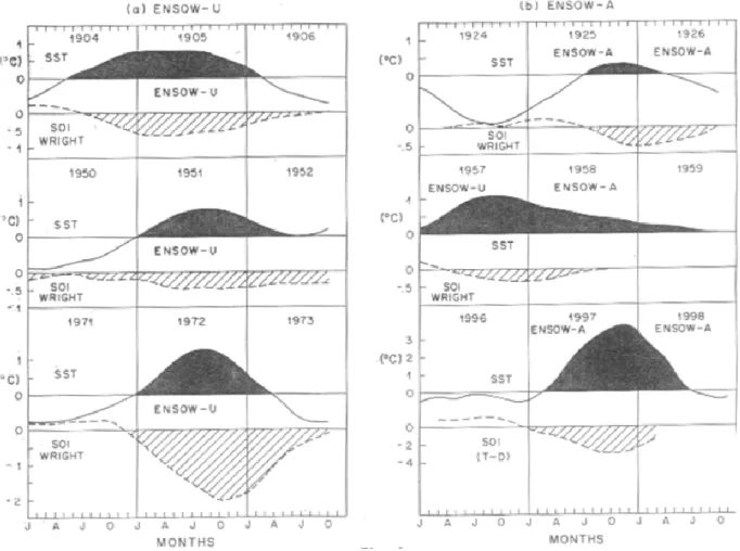
Fig. 1. Plots of 12-monthly running means of SST and SOI for selected El Nino events for 3 consecutive years, where the El Ni˜no event is
in the middle year, (a) Unambiguous ENSOW (ENSOW-U) 1905, 1951, 1972, for which SST maxima and SOI minima are in the middle of the calendar year, and (b) Ambiguous ENSOW (ENSOW-A) 1925, 1958, 1997, for which SST maxima and SOI minima are not in the middle of the calendar year.
which Unambiguous ENSOW type events (ENSOW-U, dis-cussed later on) were found to be overwhelmingly associated with droughts in India, Sri Lanka, South-eastern Australia and some other parts of the globe.
2 El Ni ˜no characteristics and their implications for rainfall
2.1 Finer classification of El Ni˜no events
The term ENSO is used nowadays for the general phe-nomenon of the El Ni˜no/Southern Oscillation. However, in our classification here, its components EN, SO are used in their literal sense. Thus, every year was examined to check whether it had an El Ni˜no EN (as listed in Quinn et al., 1978, 1987), and/or Southern Oscillation Index SOI mini-mum (SO) and/or warm (W) or cold (C) equatorial eastern Pacific sea surface temperature (SST) anomalies. For SO and SST, 12-month running means were used. Several years were ENSOW, i.e., El Ni˜no (EN) existed near Peru coast, SOI had minima (SO), and Pacific SST was warmer (W).
These were subdivided into two groups viz., Unambiguous ENSOW (ENSOW-U) where El Ni˜no existed near Peru coast and the SOI minima and SST maxima in the 12-month run-ning means were in the middle of the calendar year (May– Aug.) and, Ambiguous ENSOW (ENSOW-A) where El Ni˜no existed near Peru coast, but the SOI minima and SST max-ima were in the early or later part of the calendar year, not in the middle. Besides these, there were other El Ni˜no years of the type ENSO (El Ni˜no existed, SOI minima existed, but SST in the Pacific, away from the Peru-Ecuador coast, was neither warmer nor colder, just normal), ENW, ENC, i.e., El Ni˜no existed, SOI minima did not exist, but SST was warm W, or cold C (before or after the El Ni˜no) or just EN (i.e., El Ni˜no existed only near Peru coast, no SOI minima or cen-tral and eastern Pacific SST maxima or minima). Some other years did not have an El Ni˜no and were of the types SOW (SOI minima existed and Pacific waters were warm, but no El Ni˜no was reported by Quinn et al.), SOC, SO, W, and C, where the last category C contains all Anti-El Ni˜nos, i.e., La Ni˜nas. The types ENC or SOC look contradictory. Actually, in these years, EN and/or SO and C did not occur simulta-neously. EN or SO occurred in a part of the year and was
followed or preceded by a cold Pacific SST, i.e., C event. Years not falling into any of these categories were termed as Non-events. We have this classification ready for all years from 1871 onwards. Appendix 1 gives the classification for 1900 onwards.
Figure 1 shows the plots of the 12-monthly running aver-ages of Pacific SST (roughly, the Ni˜no 3.5 region) and the Southern Oscillation Index SOI for a few selected intervals of 3 consecutive years, the middle year being an El Ni˜no year. In Fig. 1a, SOI minima and SST maxima (12 monthly running means) are in the middle of the calendar year of the El Ni˜no year (middle part) and these are ENSOW-U (Un-ambiguous ENSOW) years. For such years, the AISM (All India Summer Monsoon) normalized rainfalls had negative deviations. Figure 1b shows similar plots for some years of the ENSOW-A (Ambiguous ENSOW) type. Here, the SOI minima and SST maxima of the El Ni˜no year (middle part) are not in the middle of the calendar year. For such years, the AISM deviations generally indicated almost normal or sometimes even excess rainfall (see below). During 1871– 1990, there were 47 El Ni˜no years. Among these, 16 could be designated as Unambiguous ENSOW, 15 as Ambiguous ENSOW and 16 as Other EN.
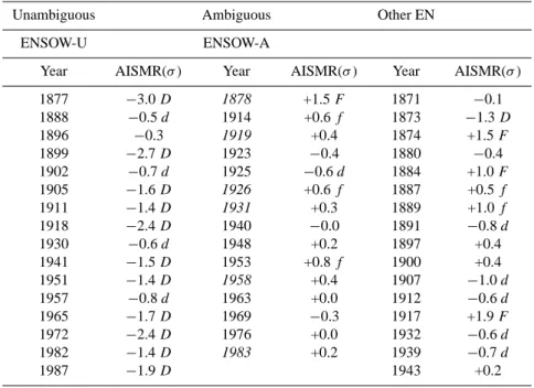
2.2 Rainfall effects in All India Summer Monsoon The various El Ni˜no years and the corresponding normal-ized AISMR (All India Summer Monsoon Rainfall) anoma-lies were as in Table 1. For AISMR, the mean and the stan-dard deviation (σ ) were calculated and the value of every year was expressed as normalized, i.e., deviation from the mean, divided by the standard deviation. These normalized deviations AISMR(σ ) were categorised as normal (no sym-bol) if these were within ±0.5σ ; f (moderate floods) and d (moderate droughts) if within 0.5 to 1.0σ and −0.5 to −1.0σ respectively; F (severe floods) if above 1.0σ and D (severe droughts) if below −1.0σ .
As can be seen, the Unambiguous ENSOW are all asso-ciated with droughts (d, D), while the Ambiguous ENSOW are mostly associated with normal rainfall. Here, the years shown in italics are II year events (1958 in 1957–1958, etc.) and it seems that these II years do not show droughts. The Other EN are associated with droughts, floods and normal rainfall.
2.3 Rainfall effects in other regions
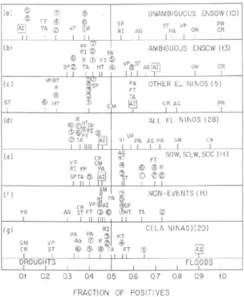
Overwhelming association of ENSOW–U with droughts or floods was observed for many other regions. The Tables will not be shown here. As a measure of the association, the fraction of positive rainfall deviations in any category of years could be considered. For example, for ENSOW-U category of 16 events, All India Summer Monsoon Rainfall had all negative deviations and the number of positive devi-ations was zero. Hence, the fraction of Positive/Total was 0.0. At other locations where there were floods, the fraction of positives would be near 1.0. Figure 2 shows the plot of
Fig. 2. Plot of positive fractions for various rainfalls for different
types of events. The central vertical line is for a fraction of 0.5, i.e., equal number of positive and negative rainfall deviations, implying poor relationship. Extreme left, droughts; extreme right, floods.
these fractions of positive deviations. It refers to regions in South America, but similar plots are available for other parts of the globe. The vertical line in the middle is for a fraction 0.5, implying equal number of positive and negative rainfall deviations and hence, a poor relationship. Regions in the left extreme have very low fractions (0.0, 0.1, 0.2) of pos-itive rainfall deviations, implying a good relationship with droughts. Regions in the right extreme have large fractions (0.8, 0.9, 1.0) of positive rainfall deviations, implying a good relationship with floods. Thus,
1. For Unambiguous ENSOW-U, a very good associa-tion is with droughts in India; Sri Lanka (southwest monsoon); Tasmania (Southeast Australia); Singapore, Brunei, Indonesia (Southeast Asia); Ceara, Rio grande do Norte, Paraiba, Pernambuco (Northeast Brazil). Also, there is good association with floods in Chile, Peru, Core Region, Gulf of Mexico and South Brazil. 2. For Ambiguous ENSOW-A and Other El Ni˜nos,
frac-tions are near 0.5, implying poor relafrac-tionships. But for Peru and Core regions, relationship with floods is good even for these events.
3. For other types of years not involving El Ni˜nos, rela-tionship is poor.
38 R. P. Kane: El Ni˜no effects on rainfall in South America
Table 1. All India Summer Monsoon Rainfall (AISMR) during El Ni˜no years of three types, Unambiguous ENSOW (ENSOW-U),
Ambigu-ous ENSOW (ENSOW-A), and Other EN.
Unambiguous Ambiguous Other EN
ENSOW-U ENSOW-A
Year AISMR(σ ) Year AISMR(σ ) Year AISMR(σ )
1877 −3.0 D 1878 +1.5 F 1871 −0.1 1888 −0.5 d 1914 +0.6 f 1873 −1.3 D 1896 −0.3 1919 +0.4 1874 +1.5 F 1899 −2.7 D 1923 −0.4 1880 −0.4 1902 −0.7 d 1925 −0.6 d 1884 +1.0 F 1905 −1.6 D 1926 +0.6 f 1887 +0.5 f 1911 −1.4 D 1931 +0.3 1889 +1.0 f 1918 −2.4 D 1940 −0.0 1891 −0.8 d 1930 −0.6 d 1948 +0.2 1897 +0.4 1941 −1.5 D 1953 +0.8 f 1900 +0.4 1951 −1.4 D 1958 +0.4 1907 −1.0 d 1957 −0.8 d 1963 +0.0 1912 −0.6 d 1965 −1.7 D 1969 −0.3 1917 +1.9 F 1972 −2.4 D 1976 +0.0 1932 −0.6 d 1982 −1.4 D 1983 +0.2 1939 −0.7 d 1987 −1.9 D 1943 +0.2
5. For C type events (La Ni˜nas), a very good association is with floods in India; and droughts in Chile, Core region, Gulf of Mexico.
2.4 Can ENSOW-U be predicted?
If the relationship with ENSOW-U is so good, it could be used for predicting extreme rainfall events, if the ENSOW-U can be predicted with some antecedence. Unfortunately, this does not seem to be possible at present with any reasonable accuracy. Take the example of the 1997–1998 El Ni˜no event. In the last two decades, many models have been developed to predict the evolution of El Ni˜no as well as the Southern Oscillation. However, instead of the predicted turning warm only in late 1997, the El Nino started early (in March 1997). As remarked by Trenberth (1998), in digesting these predic-tions in real time, it was not possible to make a forecast until about April 1997 when the SST warming became clearly evi-dent in the eastern tropical Pacific. Particulary deceptive was the forecast of the Cane-Zebiak model. This model had suc-cessfully forecast the 1986–1987 event (Cane et al., 1986; Zebiak and Cane, 1987). Hence their prediction of “normal by June 1997, warming thereafter” substantially inhibited the issuing of a forecast for March 1997.
In the Executive Summary for the La Ni˜na Summit Re-port of a Workshop held in Boulder, Colorado from 15–17 July, 1998, Glantz (1998) mentions the key points about prediction of the El Ni˜no 1997 as follows: (a) The perfor-mance in forecasting the onset of the 1997–1998 El Ni˜no was largely mediocre. (b) Dynamical models as yet do not outperform the statistical ones, with respect to forecasting El Ni˜no. (c) The communication between forecasters and users
still leaves something to be desired. It appears that neither really understands how the other thinks and what the other does or does not understand.
2.5 SST characteristics in the Pacific
The finer classification mentioned above is obtained by vi-sual examination of the plots and no physical basis is offered, except perhaps that the circulation patterns affecting rainfall operate best when these maximise in the northern summer months. However, some relationship with SST patterns in the Pacific may be involved. Fu et al. (1986) identified two dis-tinct patterns in Pacific SST, one operating in some El Ni˜no years and the other in other El Ni˜no years. Ward et al. (1994) separated years when AISM and Sahel had droughts or ex-cess rainfalls, during 1904–1990. From these, years having El Ni˜nos or La Ni˜nas were selected for analysis. The sym-bol FIT means years where rainfalls were as expected. Four categories were obtained:
– El Ni˜no Type I (FIT years): El Ni˜no years when India
and Sahel had droughts (1904, 11, 13, 25, 41, 51, 57, 63, 66, 72, 76, 77, 82, 87).
– El Ni˜no Type II (NOT FIT years): El Ni˜no years when
India and Sahel had excess rains (1912, 15, 18, 19, 23, 26, 30, 31, 32, 40, 47, 52, 53, 58, 65, 69, 83, 86, 90).
– La Ni˜na Type I (FIT years): La Ni˜na years when India
and Sahel had excess rains (1906, 09, 16, 24, 50, 54, 64, 70, 74, 75, 88).
– La Ni˜na Type II (NOT FIT years): La Ni˜na years when
India and Sahel had droughts (1908, 17, 20, 21, 28, 38, 39, 42, 43, 49, 55, 71, 73, 89).
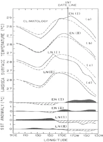
Type I were the FIT years (rainfall as expected), while Type II were the NOT FIT years. The average SST longi-tude profiles for these four groups for JAS months are shown in Fig. 3. The dashed plot shows the average pattern (clima-tology) for 1951–1980. The full lines show the average SST for El Ni˜no Type I (EN I) in the first plot, El Ni˜no Type II (EN II) in the second plot, La Ni˜na Type I (LN I) in the third plot and La Ni˜na Type II (LN II) in the fourth plot, with the climatology (dashed line) superimposed on each plot. When the climatology is subtracted, the residuals (SST anomalies) are as shown in the lower part of Fig. 3. EN I has positive SST anomalies in the longitudes 130–180 W while EN II has positive SST anomalies near 170 E. LN I has positive SST anomalies near 150–160 E and large negative SST anomalies in 130–180 W, while LN II has small positive SST anomalies near 120 E and small negative anomalies in 130–180 W.
To test whether the 1997–1998 El Ni˜no had a pattern like EN I or EN II, plots of SST anomalies were made at different longitudes 10◦ apart for JAS months for different latitude belts 4◦ apart (30 N–26 N, 26 N–22 N, ....2 N–2 S, ....22 S–26 S, 26 S–30 S). Substantial anomalies were seen in the 6 N–10 S belt, in a broad longitude around 120 W. Thus, the anomaly pattern resembled EN I pattern. As such, the 1997–1998 El Ni˜no should be of the FIT type, suitable as a “tropic-wide oscillation of boreal summer rainfall” men-tioned by Ward et al. (1994) and should have caused severe droughts in India, southeast Australia etc. However, this ex-pectation was not fulfilled for the 1997–1998 event, leaving in doubt whether the longitude distribution in Pacific SST is a deciding factor.
3 The El Ni ˜no of 1997–1998
In March 1997, an El Ni˜no developed and proved to be the strongest in the 20th century. Kane (1999a, b) has sum-marized its effects in different parts of the globe. For S. America, Southern Peru had droughts while eastern, north-ern Peru and Ecuador had floods. In Bolivia, parts adjacent to Brazil had floods while parts adjacent to Peru and Chile had droughts. In northeast Brazil, the observed rainfall for March–May 1997 (main rainy season) was 15–30% below normal. Thus, El Ni˜no effects could be claimed. In 1998, there was a very severe drought in northeast Brazil. So again, El Ni˜no effect could be claimed, though the El Ni˜no was on the decline during March–May 1998. There was intense, prolonged drought in Amazonia and Roraima (both in north-ern Brazil). By 1998 end, northeast Brazil had some rain-fall and came out of a prolonged severe drought. In South Brazil, Paraguay, Uruguay, Northeast Argentina and Chile, there were heavy rains in 1997. In Chile, deserts bloomed after 40 years. Thus, El Ni˜no effect was fully visible. North-ern Uruguay was wetter in April–July of 1998. September and October of 1998 were above normal in the southern part
Fig. 3. Plot of July-August-September average SST (full lines)
ver-sus longitude in the Pacific for El Nino years of (a) the FIT type EN(I), which favoured droughts in Sahel and India, (b) NOT FIT type EN(II), which did not favour droughts, and for La Nina years of (c) the FIT type LN(I), which favoured excess rainfall in Sahel and India, (d) NOT FIT type LN(II), which did not favour excess rainfalls (Ward et al., 1994). The dashed line superposed on each plot is the climatology. Deviations (SST anomalies) from the cli-matology are plotted in the bottom part.
of Brazil. However, November and December were below normal.
4 Conclusions
For southern S. America, Kane (2002) examined data for var-ious locations and concluded that whereas ENSOW-U events had very good association with floods, some ENSOW-A also had a good association. La Ni˜nas were mostly associated with droughts but some were associated with floods. Some non-events (neither El Ni˜nos nor La Ni˜nas) were also as-sociated with extreme rainfalls. These facts render dubi-ous the relationships of El Ni˜no and La Ni˜na with rainfalls. The Amazon river basin and its vicinity (15◦N–20◦S, 30◦– 80◦W) indicated that the rainfalls were highly variable both from year to year and from region to region. Correlations with even nearby regions hardly exceeded 0.50, though cor-relations were better (up to 0.70) in the regions near the
40 R. P. Kane: El Ni˜no effects on rainfall in South America
Table A1.
Unambiguous Ambiguous Other SOW etc. Non- C
ENSOW ENSOW El Ni˜nos events La Ni˜na
M 1902 RKP M 1914 R S 1912 ENSO 1904 SOW KP 1901 1903 K*P* M 1905 R P M 1919 II M 1929 EN 1913 SOW KP 1915 1906 K*P* S 1911 RKP M 1923 RK S 1932 EN 1944 SOW 1937 1908 K*P* S 1918 I RKP S 1925 I RKP M 1939 EN 1977 SOW 1945 1909 M 1930 I RKP S 1926 II M 1943 EN 1979 SOW 1947 1910 S 1941 II R P M 1931 II K* M 1907 ENC 1920 W K* 1952 1916 K*P* M 1951 RKP S 1940 I P S 1917 ENC 1968 W P 1966 1921 S 1957 I RKP W 1948 P S 1927 ENC 1986 W K 1978 1922 M 1965 RKP M 1953 RK S 1973 ENC 1959 SO 1980 1924 K* S 1972 I RKP S 1958 II 9 events 1974 SO 1981 1928 K* S 1982 KP W 1963 KP 1935 SOC 1984 1933 M 1987 W 1969 RKP 1936 SOC 1985 1934 12 events M 1976 RKP 1946 SOC P* 1989 1938 K* S 1983 II P* 1949 SOC K* 1990 1942 K*
14 events 14 events 14 events 1950
1954 K* 1955 P* 1956 1960 1961 1962 1964 K*P* 1967 P* 1970 K*P* 1971 1975 K* 1988 27 events
eastern coast of Brazil. Moderate relationship with ENSO indices was obtained for the Amazon river basin and the re-gions to its north, and for NE Brazil, while moderate rela-tionship with South Atlantic SST was obtained for NE Brazil and the region immediately to its west. All other relation-ships (with 30 mb wind, North Atlantic Oscillation Index, etc.) were obscure.
Appendix
Distribution of the years 1900–1990 in various categories. Symbols S (strong), M (Moderate), W (Weak) indicate the strengths of the El Ni˜nos involved. I and II indicate first and second years of double events (1957–1958 etc.). R, K, P in-dicate that these were selected as warm events by Rasmusson and Carpenter (1983), Kiladis and Diaz (1989) and Mooley and Paolino (1989). K* and P* indicate that these were se-lected as cold events by Kiladis and Diaz (1989) and Mooley and Paolino (1989).
Acknowledgements. This work was partially supported by FNDCT,
Brazil under contract FINEP-537/CT. Edited by: P. Fabian and J. L. Santos Reviewed by: J. L. Santos and another referee
References
Cane, M. A., Zebiak, S. E., and Dolan, S. C.: Experimental fore-casts of El Nino, Nature, 321, 827–832, 1986.
Deser, C. and Wallace, J. M.: El Nino events and their relation to the Southern Oscillation: 1925–1986, J. Geophys. Res. 92, 14 189– 14 196, 1987.
Fu, C., Diaz, H. F., and Fletcher, J. O.: Characteristics of the re-sponse of sea surface temperature in the central Pacific associ-ated with warm episodes of the Southern Oscillation, Mon. Wea. Rev., 114, 1716–1738, 1986.
Glantz, M. H.: A La Nina Summit: A review of the Causes and Consequences of Cold Events, Executive Summary of the work-shop, 15–17 July 1998, Boulder, Colorado, Environmental and Societal group, NCAR, Boulder, 1998.
Kane, R. P.: On the relationship of ENSO with rainfall over differ-ent parts of Australia, Aust. Met. Mag., 46, 39–49, 1997a. Kane, R. P.: Relationship of El Nino-Southern Oscillation and
Pa-cific sea surface temperature with rainfall in various regions of the globe, Mon. Wea. Rev., 125, 1792–1800, 1997b.
Kane, R. P.: Extremes of the ENSO phenomenon and the Indian summer monsoon rainfall, Int. J. Climatol., 18, 775–791, 1998a. Kane, R. P.: ENSO relationship to the rainfall of Sri Lanka, Int. J.
Climatol., 18, 859–871, 1998b.
Kane R. P.: El Ni˜no, Southern Oscillation, equatorial eastern Pacific sea surface temperatures and summer monsoon rainfall in India, Mausam, 49, 103–114, 1998c.
Kane, R. P.: Some characteristics and precipitation effects of the El Ni˜no of 1997–1998, J. Atmos. Solar-Terr. Phys., 61, 1325–1346, 1999a.
Kane, R. P.: Rainfall extremes in some selected parts of central and south America: ENSO and other relationships reexamined, Int. J. Climatol., 19, 423–455, 1999b.
Kane, R. P.: Precipitation anomalies in southern South America as-sociated with a finer classification of El Ni˜no and La Ni˜na events, Int. J. Climatol., 22, 357–373, 2002.
Kiladis, G. N. and Diaz, H. F.: Global climate anomalies associ-ated with extremes in the Southern Oscillation, J. Clim., 2, 1069– 1090, 1989.
Mooley, D. A. and Paolino, D. A.: The response of the Indian mon-soon associated with the change in sea surface temperature over the eastern south equatorial Pacific, Mausam, 40, 369–380, 1989. Quinn, W. H., Zoff, D. G., Short, K. S., and Kuo Yang, R. T. W.: Historical trends and statistics of the Southern Oscillation, El Nino and Indonesian droughts, Fish. Bull., 76, 663–678, 1978. Quinn, W. H., Neal, V. T., and Antunes de Mayolo, S. E.: El Nino
occurrences over the past four and a half centuries, J. Geophys. Res., 92, 14 449–14 461, 1987.
Rasmusson, E. M. and Carpenter, T. H.: The relationship between eastern equatorial Pacific sea surface temperatures and rainfall over India and Sri Lanka, Mon. Wea. Rev., 111, 517–528, 1983. Ropelewski, C. F. and Halpert, M. S.: Global and regional scale pre-cipitation patterns associated with El Nino/Southern Oscillation, Mon. Wea. Rev., 115, 1606–1626, 1987.
Trenberth, K. E.: The different flavors of El Nino, Proc. 18th An-nual Climate, Diagnostics Workshop, Boulder, CO, 50–53, 1993. Trenberth, K. E.: Development and forecasts of the 1997-98 El
Nino: CLIVAR Scientific Issues, Exchanges, 3, 4–14, 1998. Ward, M. N., Maskell, K., Folland, C. K., Rowell, D. P., and
Wash-ington, R.: A tropic-wide oscillation of boreal summer rain-fall and patterns of sea-surface temperature, Climate Research Technical Note CRTN48, Hadley Center, Meteorological Office, Bracknell, UK, 29pp., 1994.
Zebiak, S. and Cane, M.: A model El Nino-Southern Oscillation, Mon. Wea. Rev., 115, 2262–2278, 1987.