Super Earths Using an All-Sky Transit Survey and
Follow-up by the James Webb Space Telescope
The MIT Faculty has made this article openly available. Please share how this access benefits you. Your story matters.Citation Deming, D. et al. “Discovery and Characterization of Transiting Super Earths Using an All-Sky Transit Survey and Follow-up by the James Webb Space Telescope.” Publications of the Astronomical Society of the Pacific 121.883 (2009): 952–967.
As Published http://dx.doi.org/10.1086/605913
Publisher University of Chicago Press, The
Version Author's final manuscript
Citable link http://hdl.handle.net/1721.1/74029
Terms of Use Creative Commons Attribution-Noncommercial-Share Alike 3.0
arXiv:0903.4880v2 [astro-ph.EP] 3 Aug 2009
James W ebb Space T elescope
D. Deming1 , S. Seager2 , J. Winn3,4, E. Miller-Ricci5 , M. Clampin6 , D. Lindler7 , T. Greene8 , D. Charbonneau5 , G. Laughlin,9 , G. Ricker4 , D. Latham5 , & K. Ennico8 Received ; accepted Submitted to PASP 1
Solar System Exploration Division, Goddard Space Flight Center, Greenbelt, MD 20771
2
Department of Earth, Atmospheric & Planetary Sciences, and Department of Physics, Massachusetts Institute of Technology, 77 Massachusetts Ave,
Cambridge MA 02139-4307
3
Department of Physics, Massachusetts Institute of Technology, 77 Massachusetts Ave, Cambridge MA 02139-4307
4
Kavli Institute for Astrophysics and Space Research, Massachusetts Institute of Technology, 77 Massachusetts Ave, Cambridge MA 02139-4307
5
Harvard-Smithsonian Center for Astrophysics, Cambridge MA 02138
6
Exoplanet and Stellar Astrophysics Laboratory, Goddard Space Flight Center, Greenbelt MD 20771
7
Sigma Scientific Corporation, Goddard Space Flight Center, Greenbelt MD 20771
8
Space Science Division, Ames Research Center, Moffett Field CA 94035-1000
9
ABSTRACT
Doppler and transit surveys are finding extrasolar planets of ever smaller mass and radius, and are now sampling the domain of superEarths (1 − 3R⊕).
Recent results from the Doppler surveys suggest that discovery of a transiting superEarth in the habitable zone of a lower main sequence star may be possible. We evaluate the prospects for an all-sky transit survey targeted to the brightest stars, that would find the most favorable cases for photometric and spectroscopic characterization using the James Webb Space Telescope (JWST). We use the proposed Transiting Exoplanet Survey Satellite (TESS) as representative of an all-sky survey. We couple the simulated TESS yield to a sensitivity model for the MIRI and NIRSpec instruments on JWST. Our sensitivity model includes all currently known and anticipated sources of random and systematic error for these instruments. We focus on the TESS planets with radii between Earth and Neptune. Our simulations consider secondary eclipse filter photometry using JWST/MIRI, comparing the 11− and 15 µm bands to measure CO2 absorption
in superEarths, as well as JWST/NIRSpec spectroscopy of water absorption from 1.7− to 3.0 µm, and CO2 absorption at 4.3 µm. We find that JWST will be
capable of characterizing dozens of TESS superEarths with temperatures above the habitable range, using both MIRI and NIRspec. We project that TESS will discover about eight nearby habitable transiting superEarths, all orbiting lower main sequence stars. The principal sources of uncertainty in the prospects for JWST characterization of habitable superEarths are superEarth frequency and the nature of superEarth atmospheres. Based on our estimates of these uncertainties, we project that JWST will be able to measure the temperature, and identify molecular absorptions (water, CO2) in 1 to 4 nearby habitable TESS
1. Introduction
In the quest to measure the spectrum of a habitable exoplanet, the observer must successfully disentangle the planetary flux from that of the central star. Two methods are currently in use for the direct study of gas-giant exoplanets, and practitioners of each are working to apply these methods to the study of rocky exoplanets. In the first technique, the planet and star are separated spatially through high angular resolution imaging (Kalas et al. 2008; Marois et al. 2008). This method favors systems wherein the angular separation is as large as possible. The second method obviates the need for high angular resolution imaging by studying the combined light of the planet and star in transiting systems. In these systems, the planet and star undergo periodic mutual eclipses (see Charbonneau et al. 2007 for a review), and the emission from each is subsequently separated with the knowledge of the previously-characterized orbit. The primary disadvantage of the latter approach is obvious: only a small fraction of exoplanets will have their orbits aligned so as to undergo eclipses as viewed from the Earth.
The transit method offers several advantages that motivate its further study. The first is that of technological simplicity, since it does not require the development of extreme-contrast ratio direct imaging. The second is that of scientific impact: eclipsing systems, for which the photometric transit and stellar radial velocity orbit have been observed, permit a geometric determination of the planetary radius and a dynamical estimate of the planetary mass by a means that is virtually free of astrophysical assumption. For such systems, the interpretation of the hemisphere-averaged spectrum is likely to be more scientifically fruitful than for systems lacking direct measurements of the masses or radii. For example, without a knowledge of the planet radius, there exists a degeneracy between the emitting area and surface flux (see e.g., Kalas et al. 2008). More generally, the bulk composition and physical structures of transiting exoplanets are likely to be well
constrained, and inferences about the atmosphere (for example, its chemical composition) are likely to be far more penetrating than for cases in which only the spectrum is available.
Over the past 7 years, the characterization of the atmospheres of Gyr-old planets orbiting solar peers has proceeded rapidly and exclusively through the study of combined light of the planet and star in transiting systems. A partial list of such successful studies includes Charbonneau et al. (2002, 2005, 2008), Deming et al. (2005, 2006, 2007), Grillmair et al. (2007, 2008), Harrington et al. (2006, 2007), Knutson et al. (2007, 2008, 2009), Richardson et al. (2007), Swain et al. (2008, 2009), Tinetti et al. (2007), and Vidal-Madjar et al. (2003). All of the detections listed in the previous sentence were accomplished with either the Hubble Space Telescope or Spitzer Space Telescope, two general purpose, space-based facilities, neither of which were optimized for exoplanet studies (indeed, these studies were not anticipated during the development of either facility).
Since there is currently intense interest in rocky superEarth exoplanets,1
it is desirable to explore the factors that will limit their discovery and study using transit/eclipse methodology. We consider the coming James Webb Space Telescope (JWST) and ask what it could accomplish for studies of the atmospheres of transiting exoplanets, especially for smaller, rocky, and potentially habitable worlds. We note that neither Hubble nor Spitzer served as the discovery observatory for the planets they characterized: rather, the tasks of discovery and characterization were split, with ground-based surveys pursuing the former and these two spacecraft conducting the latter. Similarly, we anticipate that JWST will be able to undertake characterization studies of the atmospheres of habitable worlds, but only if these objects are identified in nearby, transiting systems by a separate discovery effort. Since the most favorable systems are the closest ones, and very high photometric precision is needed for long time periods, a bright star, all-sky, space-borne survey such as
1
the proposed Transiting Exoplanet Survey Satellite (TESS) is the natural starting point for our study.
The specific purpose of this paper is to evaluate the potential for discovery and characterization of exoplanets by using an all-sky transit survey and JWST follow-up. Our simulation includes planets ranging in size from Earth to Jupiter. JWST follow-up of Jupiter-size transiting planets would be of enormous scientific utility. Nevertheless, we here focus on planets of Neptune size and smaller. Our analysis includes ‘hot superEarths’ as well as those in the habitable zone (HZ)2
. We evaluate whether the sources of uncertainty for superEarth discovery and characterization are primarily astrophysical (e.g., occurrence rate for superEarths), or technological (sensitivity of instrumentation and surveys). Our evaluation begins by projecting the yield of TESS. Although TESS is still at the proposal stage, it provides the most well-studied basis from which to project the yield of a space-borne, bright star, all-sky, transit survey. We couple the TESS planets to sensitivity calculations for specific observing modes of the Near-Infrared Spectrograph (NIRSpec) and Mid-Infrared Instrument (MIRI) instruments on JWST. Our intent is not to define and compare the relative merits of all potential modes of JWST exoplanet observations. Instead, we concentrate on the likely success for exoplanet characterization using two of the most obvious observational modes.
Potential JWST exoplanet transit observations have been discussed by several authors (Clampin et al. 2009; Greene et al. 2007; Kaltenegger & Traub 2009; Lunine et al. 2008; Seager et al. 2008; Valenti et al. 2005, 2006; Valenti 2008). Our treatment here goes beyond previous work in that we specifically include simulations of an all-sky survey, coupled to a characterization simulation that includes the JWST’s pointing constraints (field-of-regard),
2
We use the term habitable to be synonymous with a thermal equilibrium temperature range of 273 to 373 Kelvins, with no other requirements.
and anticipated JWST instrument- and detector-related systematic errors, based on experience with Spitzer and current engineering data from the JWST instruments.
Sec. 2 presents an estimate of the likely distance to the closest transiting habitable exoplanet, and Sec. 3 describes our statistical model for the yield of TESS. Sec. 4 discusses a simple model for exoplanet characterization using transits and eclipses, and later sections develop more exhaustive simulations of JWST characterization of TESS planets: Sec. 5 gives our sensitivity and noise models for the JWST instruments, and Sec. 6 applies these noise models to the TESS planets. Sec. 7 gives our conclusions and comparisons to other work.
2. The Closest Transiting Habitable Exoplanet
It is of interest to consider the probable distance of the closest habitable planet that transits, assuming that we discover all nearby transiting planet systems. The probability of a transiting habitable planet within distance d can be calculated from the space density of nearby stars, if we know the distribution of planets vs. orbital size for each stellar spectral type. Because these distributions are not securely known, we adopt a very general assumption. We assume that a fraction f of stars host exactly one planet in their HZ, and we place half of them at the inner HZ boundary, and half at the outer HZ boundary.
The probability of at least one transiting planet within a sphere of radius d centered on the Sun equals 1 −Q
ipi, where pi is the probability that no planet transits star i, and
i indexes the stars within distance d. Given the above assumptions on the orbital radii of the planets, and the transit probability for each planet (Rstar/a), this is a straightforward
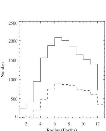
calculation. We adopt circular orbits, and the stellar space densities versus spectral type described in Sec. 3. The results are shown in Figure 1 for planet frequencies of f = 1.0, 0.3
and 0.1. This calculation shows that if every star hosts a planet in the HZ, then the closest transiting habitable planet is likely (i.e., probability 0.5) to be found at d = 5 pc. This distance increases to d = 7 and 10 pc for f = 0.3 and 0.1. Moreover, even for a HZ frequency as low as f = 0.01 per star, the probable distance for the nearest example (not illustrated) is d = 22 pc. These calculations suggest good prospects for JWST characterization even if HZ planets are moderately scarce. However, there remains the practical problem of whether a given transit survey such as TESS can necessarily find the nearest examples.
3. Yield of an All-Sky Transit Survey
We here simulate the yield of an all-sky survey targeted primarily to bright (V < 13.5) stars, and we elaborate on how the superEarth yield of such a survey depends on superEarth occurrence and orbital distribution properties. We use the TESS survey (Ricker et al. 2008) as a practical example of an all-sky bright star survey capable of detecting transiting superEarths. TESS is proposed to view the sky from near-Earth equatorial orbit, using an array of 6 wide-field (18 × 18 degree) refractive CCD cameras on a single spacecraft. TESS monitors 2.5 × 10⁶
bright (V < 13.5) stars, with special attention to lower main sequence stars. During each orbit, TESS will monitor a 72-degree strip of right ascension, using several pointings. Each star in the TESS catalog will be monitored for at least 72 days. Since TESS requires two transits to identify a planet, it is insensitive to orbital periods exceeding 72 days.
3.1. Making Transiting Planets
Our Monte-Carlo model of the planets to be found by TESS considers main sequence host stars from spectral types F5 through M9. We adopt the absolute visual magnitude vs.
spectral type relation from Henry et al. (1994), and the main sequence luminosity function from Reid & Hawley (2000). We convert spectral type to Tef f, stellar mass and radius,
using Table 4.1 of Reid & Hawley (2000).
We make planets by first generating a set of Monte-Carlo stars in a cubical volume of 20003
pc3
centered on the Sun. This cube is larger than the TESS search space and it contains all planets that TESS will find. We assign galactic coordinates (X, Y, Z) to each star by placing them randomly within this cube, constrained by their space densities at Z=0 vs. spectral type, and enforcing an exponential distribution in height above the galactic plane (Z), with 200 pc scale height. Since transiting planets require mass measurements via high precision radial velocities, we eliminate the visually faintest stars (having V > 13.5), but we keep all stars at distances closer than 35 pc (Charbonneau & Deming 2007), regardless of their visual magnitude. Planet-hosting M-dwarfs can lie at close distances and still be visually faint, because their spectral energy distribution peaks in the IR. We reason that superEarths transiting nearby M-dwarfs will be so important that their radial velocities will be measured by some means, regardless of their visual magnitude. For example, IR spectroscopy could be used when it is sufficiently developed to achieve the precision needed for superEarths (Blake et al. 2007).
We assign exactly one planet to each star. We use various simple distribution formulae for orbital size and planetary radius, because the actual distributions are poorly known. An important rationale for our work is to define the expected yield of superEarths under various orbital size distributions. Our default distribution in orbital size uses a uniform probability density in log(a′
), where a′
= a (L⊙/L∗)
1/2, between 0 and −1.3 in log(a′
). One rationale for the stellar luminosity scaling factor is that it produces a more compact planet distribution orbiting low-mass stars, consistent with evidence for close-in planet formation in some M-dwarf planetary systems (Forbrich et al. 2008). Also, this scaling puts the same
number of planets in each temperature zone, and is a natural way to cast the problem when interested in the HZ. At the opposite extreme, we also explore the effect of a distribution whose probability density for orbital size is uniform in a.
Because the magnitude of the transit signal depends on the radius of the planet, we use radius as the independent variable in our planet distributions. We distribute planet radii (Rp) with a uniform probability density in log(Rp/R⊕), between limits of 0 and 1.1 in
the log (these limits correspond to Earth and Jupiter-sized planets, respectively). Surface gravity is needed for subsequent simulations (Secs. 5 & 6). To that end, we calculate the mass from the radius by assigning a bulk composition, and inverting the mass-radius relations of Seager et al. (2007). When R > 2R⊕, we use an icy bulk composition (ocean
planets), and when R > 3R⊕ we add a H-He envelope having a depth of 1R⊕. Planets
having radii Rp < 2R⊕ are assigned bulk compositions of either Earth-like (silicate), or
Mercury-like, with equal probability. Using this radius distribution, approximately 40% of the simulated planets are superEarths (defined by TESS as having R≦ 3R⊕).
For each planet, we calculate whether it transits based on random selection in proportion to the transit probability. Transit probability is the ratio of the stellar radius to the planet’s orbital radius, and we used circular orbits for all planets. Using circular orbits is conservative, because transit probability increases for eccentric orbits (Barnes 2007). We also assign a random impact parameter to each transit, uniformly distributed between zero and unity. From the impact parameter, we calculate the duration of each planet’s transit. Finally, we calculate the temperature of each planet, based on its orbit radius and stellar luminosity, scaling from a 287K value at 1 AU with solar luminosity.
3.2. Finding Transiting Planets
In deciding whether TESS will discover a particular transiting planet, we take the duty cycle and sensitivity of the mission into account. TESS will observe a given location in the sky once per 96-minutes, for 72 days. For each transiting planet, we calculate the in-transit times from the planet’s orbital period, assigning a random phase. We then tabulate the number of transits that overlap the TESS observing cadence, using a 10-minute time resolution. Those planets seen by TESS during at least two transits are counted as detected, providing they meet the SNR requirement.
To calculate the observed SNR of each transit, we used Phoenix model atmospheres (Hauschildt et al. 1999) for stars of each spectral type, and derived the flux incident at the TESS telescopes. The flux into the 84.6 cm2
effective collecting area of the TESS telescopes (including optics throughput and detector quantum efficiency) was integrated over the 600-1000 nm bandpass of the TESS detectors, to establish a count rate for each transiting system. Given the duration of the transit, we calculate the photon-limited SNR for the aggregate of the phased transits, and we require SNR for the transit depth to be at least 7. We also eliminate planets having transit depths less than TESS’s estimated systematic noise floor (100 ppm).
It is of interest to determine whether a mission in near-Earth orbit like TESS has an adequate sampling cadence to find transits, or whether it misses many. In our simulation, only a very small fraction of planets (<< 0.1%) exhibiting more than two transits within the 72-day TESS observing period were missed because of sampling. Those few cases include grazing transits of short period planets orbiting small stars, where the transit duration was brief (typically 30 minutes). With short transit durations, a small fraction can be resonantly out of phase with the TESS 96-minute sampling interval, but the number of such cases is negligible.
We used the above simulation procedures to produce a Monte-Carlo realization of the TESS yield, adopting a frequency of one planet per star. The real planet frequency will differ from unity, but our results are linearly scalable to other values.
3.3. Distribution of Planets and Implications
Figure 2 shows the number of planets that TESS should find, versus their radii (Rp), under two different assumptions concerning their orbital sizes. Using our default
distribution of orbit sizes, scaling with a′ (see above), TESS finds 16,244 planets. The radii of the detected planets peak just above the exoNeptune regime, at 6 R⊕. We believe that
our default distribution for a is a resonable estimate. But using a distribution of orbital size that is uniform in a, the number of detected planets drops to 6845, a factor of 2.4 less. The decrease is relatively independent of planet radius, and occurs because a uniform distribution in a overweights larger orbital sizes compared to a uniform distribution in log a′. Larger orbital sizes translate to smaller transit probabilities, and thus the yield of the survey is reduced.
The total number of small planets detected is greatly affected by the photometric sensitivity of the survey. Our default radius distribution has uniform probability density in the logarithm of Rp, and that distribution (not illustrated) slopes downward on Figure 2,
with more planets occurring in bins at small radius. But many of those small planets orbit relatively distant faint stars, and are not detected by TESS because their transits are not measured to the requisite SNR. For example, our default distributions produce 7857 transiting superEarths with radii between 2 and 3 R⊕. TESS’s total for the 2- to 3 R⊕ bin
is 409 out of the 7857 due to incompleteness at the largest distances. (TESS is flux-limited, and is not designed to be a volume-limited survey.) The total yield of superEarths from an all-sky transit survey is extremely sensitive to the light grasp and photometric precision
of the survey, to a greater extent than uncertainties involving the superEarth orbital size distribution. For gas-giant planets, SNR is not a limiting factor. Instead, the number of transiting giant planets detected is sensitive to their orbital architecture, and to galactic structure.
Finally, we evaluated the effect of visual vs. IR brightness for M-dwarfs. Our default simulation of TESS finds 320 superEarths within 35 pc of the Sun, regardless of their star’s visual magnitude. If we strictly require V < 13.5 on the grounds that radial velocity confirmation would have to be done in the visible spectral range, then the number of TESS superEarths within 35 pc drops to 90. This implies that TESS is efficient for M-dwarf transits due to its bandpass extending to 1000 nm. It also implies that successful development of precision IR radial velocity techniques may significantly increase the number of confirmed superEarths from a transit survey of bright stars.
3.4. Completeness of TESS for Nearby Transiting Habitable SuperEarths
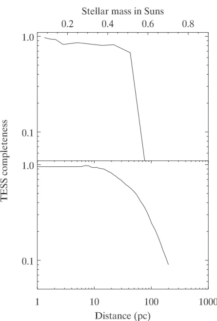
The potential discovery of habitable superEarths from the TESS survey is of special interest. We calculated the completeness of TESS for superEarths (1 − 3R⊕) by running
our Monte-Carlo simulation 500 times, and tabulating the fraction of habitable superEarths that TESS finds versus stellar mass and distance. The top panel of Figure 3 shows the completeness of TESS for transiting habitable superEarths vs. stellar spectral type, in a volume out to 35 pc. All of the habitable superEarths found by TESS orbit M-dwarfs. The completeness of TESS for M > 0.5M⊙ drops steeply because the habitable zone moves to
longer orbital periods, where TESS does not sample two transits. Although TESS misses habitable superEarths orbiting stars more massive than about 0.5M⊙, it efficiently finds
the transiting habitable superEarths nearest to our Sun. The completeness of TESS versus distance, including stars of all spectral types, is shown in the lower panel of Figure 3.
TESS completeness is 93% at 10 pc, 80% at 20 pc, and 62% at 35 pc. It falls steeply at greater distances. The high completeness at near distances is consistent with the fact that the nearest stars are predominately M-dwarfs. TESS misses the few transiting habitable superEarths that orbit stars more massive than about 0.5M⊙. These misses are few in
number because such stars have lower space densities than M-dwarfs, and planets in their habitable zones have lower probabilites to transit compared to M-dwarf habitable planets.
4. Overview of SuperEarth Characterization via Transits
The characterization of transiting exoplanets relies primarily on observations at transit (planet partially eclipsing star) as well as secondary eclipse (star eclipsing planet). Besides the mass and radius determined from transit photometry (e.g., Charbonneau et al. 2006; Winn et al. 2008), the atmosphere can be characterized via its transmission spectrum during transit (Charbonneau et al. 2002; Redfield et al. 2008; Tinetti et al. 2007; Swain et al. 2008) and the emergent atmospheric spectrum can be measured using photometry and spectroscopy at secondary eclipse (Charbonneau et al. 2005, 2008; Deming et al. 2005, 2006; Harrington et al. 2007; Knutson et al. 2008; Richardson et al. 2007; Grillmair et al. 2007, 2008). To estimate the sensitivity limits for these techniques as applied to superEarths, it is useful to first consider a simple characterization model. In this initial model, we assume that both the planet and star radiate as blackbodies. Some exoplanet atmospheric models predict that the atmospheric annulus of a transiting exoplanet will be opaque in the strongest lines over a height range of ∼ 5H (Seager & Sasselov 2002; Miller-Ricci et al. 2009), where H is the pressure scale height. Hence we approximate the magnitude of transit absorption, relative to a transparent continuum, as being equal to the area of an annulus of height = 5H. If the atmosphere is opaque over fewer scale heights, then the SNR in this simple model would be reduced in direct proportion. We calculate H using
a temperature of 323K, and a mean molecular weight of 22. These parameters are in an intermediate range for superEarths: the temperature is mid-way between the freezing and boiling point of water, and the atmospheric mean molecular weight is intermediate between free-hydrogen-rich and free-hydrogen-depleted (e.g., pure carbon dioxide) atmospheres (Miller-Ricci et al. 2009). Both this initial calculation, as well as our more detailed simulations (Secs. 5 & 6), adopt cloud-free atmospheres. We here use a superEarth mass of 10 M⊕, and a ‘dirty ocean planet’ bulk composition, intermediate between rocky and
icy. Using the mass-radius relations given by Seager et al. (2007) yields a planet radius of 2.3 R⊕. The depth of secondary eclipse is approximated as the planet-to-star area ratio,
times the ratio of Planck functions.
In analogy with Hubble Deep Field investigations (Gilliland et al. 1999), JWST characterization of a habitable superEarth would justify a large allocation of observing time, covering many transits and eclipses. We here adopt a total observation time of 200 hours. Calculation of signal-to-noise ratio (SNR) for each transit and eclipse observation requires accounting for the uncertainty of the out-of-transit (or eclipse) baseline flux level. However, for the most interesting cases (i.e., habitable planets) the orbit periods are relatively long compared to hotter planets. Habitable planet observations will be limited by the number of transits that are visible to JWST within its 5-year mission, not limited primarily by total observing time in hours. We therefore calculate the SNR using the condition that the 200 hours applies only to the in-transit/eclipse period, and that additional time will be available to measure baselines to a precision that does not significantly increase the error of the results.
Since we are here concerned with relatively nearby stars observed with a large-aperture space telescope, the observations are in the high-flux limit and we expect the dominant random noise source to be the photon noise of the host star and thermal background
radiation, and we include these noise sources for this zeroth order model in the same detail as for our full MIRI and NIRSpec noise models (Secs. 5 & 6). We adopt a telescope collecting area of 25 m2
, and an end-to-end efficiency (electrons out/photons in) of 0.3 (typical for Spitzer and expected for JWST).
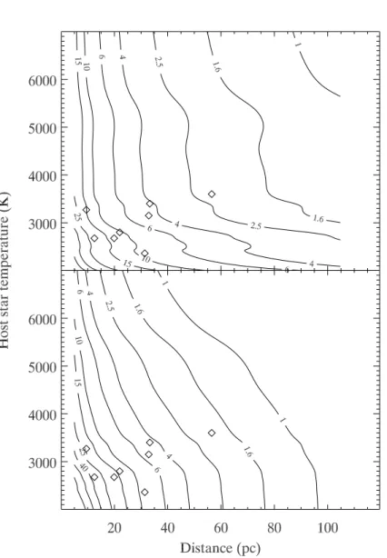
Figure 4 shows the results from this zeroth order calculation, as contours of constant SNR versus the distance to the system and the temperature (hence, mass and radius) of the host star. Transmission spectroscopy is more favorable at shorter wavelengths, because the transmission signal is proportional to the intensity of the stellar disk. We used water absorption at 2 µm for the top panel of Figure 4. We summed the FWHM of several strong bands in model transmission spectra (Miller-Ricci et al. 2009) as an estimate of the number of wavelength points (160) that would be optically thick over 5H in height. This signal is detectable to SNR ∼ 10 for systems out to ∼ 12 pc, for a wide range of stellar temperatures. Moreover, the SNR contours bulge outward to higher SNR for the lower main sequence, showing the ‘small star effect’ (Charbonneau & Deming 2007). The lower panel of Figure 4 gives the SNR for secondary eclipse photometry at 15 µm, near the peak of the planet’s thermal emission. Detection of the secondary eclipse to SNR ∼ 10 requires a distance closer than 10 pc for hotter stars, but the small-star effect extends SNR ∼ 10 to ∼ 30 pc for cooler stars like M-dwarfs.
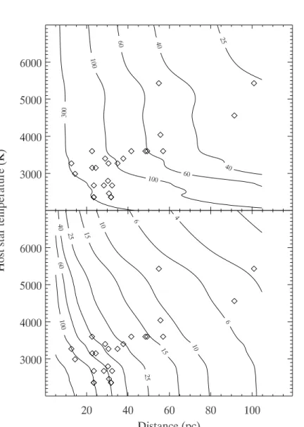
Figure 5 shows the results from our zeroth order model in the case where we raise the planet’s temperature to T = 500K, increase the mass to 20 M⊕, and lower the mean
molecular weight of the atmosphere to 2.3 (hydrogen-helium composition, with oxygen at solar abundance). This planet is a ‘hot superEarth’, and the SNR for its characterization is considerably more favorable than for habitable superEarths.
We have overplotted some examples of TESS planets on Figure 4, extracting those planets that closely bracket the parameters assumed in generating the SNR contours. For
Figure 4, we overplot the TESS planets having R = 2.3 ± 1.0 R⊕, and T = 323 ± 50 K,
i.e., habitable superEarths. For Figure 4, TESS finds 5 habitable superEarths that could be characterized by NIRSpec to SNR ∼ 10 or greater. A similar number of habitable superEarths could be characterized by MIRI secondary eclipse photometry. For Figure 5, TESS finds many more hot (T ≥ 500K) superEarths, and we have overplotted examples of these. As we will see in later Sections, these numbers are in reasonable agreement with much more exhaustive calculations.
5. Sensitivity and Noise Models for JWST Instruments
JWST is well suited to transiting planet characterization (Clampin et al. 2009). It will orbit at the L2 Lagrangian point, where continuous observations will be possible without significant blocking by the Earth. The telescope will experience a favorable thermal environment, with low background emission. Engineering studies have defined the pixel response functions, and have developed a stringent error budget for pointing jitter. Moreover, JWST instruments will incorporate direct-to-digital detector readouts, with minimal suceptibility to electrical interference. We have utilized JWST Preliminary Design Review engineering estimates of telescope performance, to couple our TESS yield calculations to simulations of JWST superEarth characterization.
Our simulations specify that JWST will observe all transits and eclipses of a given planet that are possible in principle during its 5-year mission (Gardner et al. 2006; Clampin 2008). The rationale is that the maximum number can be objectively calculated, and readers can scale the SNR for smaller programs as they deem appropriate. The maximum number of transits/eclipses is particularly large for the hotter planets, and scaling will show they can be observed to good SNR with far below the maximum number of transits.
Since the galactic coordinates of each Monte-Carlo planetary system are tagged by our simulation, we transform to ecliptic coordinates and thereby calculate the time that each individual system is available in the JWST field-of-regard. We simulate each of the observable transits/eclipses, and we specifically include non-white noise sources during observations of each transit/eclipse. However, we expect that the aggegate SNR for observations of multiple events will be proportional to the square root of the number observed, because each event is a relative measurement (in-transit/eclipse compared to out-of-transit/eclipse), and the various transits/eclipses are independent. Hence our results can be adjusted to less complete observational programs by scaling the aggregate SNR in proportion to the inverse square-root of the number of events that are actually observed.
In order to accurately evaluate the limits of characterization by JWST, we must construct a realistic noise model for the observations. In so doing, we draw on experience of Spitzer exoplanet programs, and current engineering error budgets and data for the JWST instruments, to simulate some effects that are forseeable for each JWST instrument. We concentrate on two of the many possible modes of JWST observation, namely filter photometry at secondary eclipse using MIRI, and transmission spectroscopy at transit using NIRSpec.
5.1. MIRI
JWST’s Mid-Infared Instrument (MIRI, Wright et al. 2004) will be the primary resource for exoplanet secondary eclipses, since it covers the 5− to 28 µm wavelength range where secondary eclipse contrast is maximized. MIRI will provide filter imaging, low resolution grism spectroscopy (R ∼ 100), and medium resolution spectroscopy (R ∼ 2000). We have concentrated our noise model on imaging filter photometry, rather than MIRI spectroscopy, because we want to explore a photometric technique in addition to
spectroscopic observations. This choice is conservative, because recording all wavelengths simultaneously could in principle give MIRI spectroscopy a factor of two improvement over photometric characterization.
Our MIRI noise model includes thermal background emission from the instrument, telescope, and sun shade, as calculated by Swinyard et al. (2004), as well as zodiacal thermal emission from our own solar system using the best available model (Kelsall et al. 1998) for the dependence on ecliptic latitude. We adopt a detector Fowler-8 read noise of 20 electrons per pixel, and we include 0.03 electrons/sec/pixel dark current. We use a total reflectivity for the telescope optics of 0.88, and a transmittance of 0.52 for the MIRI instrument optics including the filters. The transmission curves of the MIRI filters are not yet available, but we include the requirement on their peak transmittance (> 0.75) in the optics throughput, and we use square bandpass functions matching their required FWHM. We use detector quantum efficiencies of 0.5 and 0.6 at 11 and 15 µm, respectively (Swinyard et al. 2004).
Our JWST noise model also includes an anticipated source of systematic error, based on Spitzer experience. The Si:As detectors that will be used in JWST/MIRI are similar to those in Spitzer/IRAC, and JWST will have pointing jitter like Spitzer, but projected to be of smaller amplitude. Hence, high-precision Spitzer photometry at 8 µm provides our best current proxy for systematic errors in JWST/MIRI photometry.
Spitzer exhibits a periodic oscillation in pointing, with a 1-hour period and tens of milli-arcsec amplitude. This pointing error dithers the stellar image with respect to the detector pixels. Since the relative response of each pixel is imperfectly known (i.e., there are inaccuracies in the flat-fielding), the pointing oscillation causes an intensity oscillation in aperture photometry. Assuming (conservatively) that the MIRI flat-fielding is not improved over Spitzer, we can use the Spitzer data to calculate the magnitude of this systematic error
for MIRI photometry. This requires modeling some recent Spitzer data before turning our full attention to JWST/MIRI.
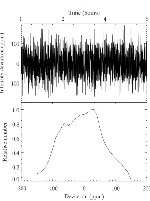
We developed a numerical model that simulates this effect. For the Spitzer data, we calculate the Fourier power spectrum of the Seager & Deming (2009) data, shown in Figure 6. This spectrum shows a peak at a period of slightly more than 1 hour, close to the known period of the telescope oscillation. The power in this peak is 1.1% of the power integrated over all frequencies, hence the amplitude of the 1-hour oscillation in intensity at 8 µm is 0.0111/2
σ = 0.105σ, where σ is the standard deviation of the intensity time series. We know the amplitude of pointing oscillations at this frequency, from measuring the stellar image displacement in the Seager & Deming (2009) data. The link between pointing oscillation and intensity oscillation is the imperfect pixel-to-pixel flat-fielding. Hence we have sufficient data to determine the magnitude of pixel-to-pixel flat-fielding error for Sptizer/IRAC.
Our numerical model resamples Spitzer’s 8 µm PSF to 10 times finer spacing, and convolves it with a simulated detector grid, also resampled to 10 times finer spacing. We do the convolution at a series of pointing values, simulating the pointing oscillation in synthetic time series photometry. The model includes flat-fielding errors on the scale of the actual IRAC pixels, with the error per pixel assigned from Gaussian random errors of a specified amplitude. We vary that amplitude until the standard deviation of the simulated time series photometry matches the observed amplitude in intensity inferred from the Fourier analysis described above. On this basis, we estimate the IRAC flat-fielding error at 8 µm to be 0.4%. We use that value in our MIRI noise model.
Our MIRI noise model adopts a PSF from a ray-traced optical model of the telescope plus instrument, for a central field location (S. Ronayette, private communication). This PSF is polychromatic, i.e., it is based on multiple wavelength samples over the 12.8 µm
filter bandpass. We spatially stretch it to represent the PSF at other wavelengths. The properties of the JWST pointing jitter can be anticipated from the engineering requirements (Ostazewski & Vermeer 2007). The telescope body pointing is controlled at a 16 Hz sampling rate, with a 0.02 Hz bandwidth. The fine guidance sensor is also sampled at 16 Hz, with a 0.6 Hz bandwidth. The 1σ amplitude of pointing jitter above the control bandwidth is 4.2 milli-arcsec (mas) per axis, and within the bandwidth it is 5.1 mas per axis. Uncontrolled drift is specified to be less than 2.2 mas per axis in a 10,000-second science exposure. We model the jitter within and above the control bandwidth as Gaussian random error of the specified magnitude, and we model the uncontrolled drift as monotonic and linear in time (worst case). This produces a 1σ deviation of 7 mas per axis for a 10,000-second exposure. We note that exoplanet observers find a monotonic drift of much larger amplitude (∼ hundreds of mas) in Spitzer pointing over ∼ tens of hours.
We use the above attitude control properties to generate pointing errors for a long time series of synthetic MIRI photometry. We adopt highly oversampled (100x) realizations of the MIRI detector grid and the PSF. The detector grid has 0.4% uncompensated response variation per original pixel. We shift the PSF relative to the detector grid, in accord with the synthetic pointing errors, multiply by the pixel sensitivities, and sum spatially to produce synthetic aperture photometry that contains only this error source. We model this error using a 10-second time resolution, but the actual exposure time for bright stars may be shorter than 10-seconds. Our noise model implicitly assumes that short exposures can be co-added (on the ground) to 10-second resolution, with no loss except for the increased overhead entailed by frequent detector reading (see below).
Noise from a representative 6-hour set of 10-second exposures, is shown in Figure 7. We generated a 200-hour times series using this methodology, and we draw a sequential portion of that noise reservoir, starting at a random time, when modeling each eclipse
for each planet. Figure 7 includes the histogram of modeled intensity fluctuations. This histogram is distinctly non-Gaussian, but the amplitude of this error source is generally small (< 10−4
). Although JWST has a higher spatial resolving power than Spitzer (tending to increase this error), it also has much finer pixel scale, and much better telescope pointing control, which greatly reduces this source of photometry error.
Some planets will orbit bright stars, filling the MIRI detector in less than a 10-second exposure time. These systems require increased overhead to read-out the detector frequently in subarray mode. We calculate the exposure time required for each planet-hosting star to fill the brightest pixel to 105
electrons (Wright et al. 2004). Our noise model includes a 50 msec overhead per subarray read, and thereby accounts for the observing efficiency.
5.2. NIRSpec
The principal use of NIRSpec for transiting exoplanets will be to measure the transmission spectrum of their atmospheres during transit. We have modeled observations of transit water absorption in the 1.6− to 3 µm region, and CO2 absorption near 4.3 µm,
as observed using slit spectroscopy at a spectral resolving power R = 1000. The optical design of NIRSpec has been discussed by Kohler et al. (2005). Our model adopts a total optical transmission for the NIRSpec optics after the slit of 0.4, and we also include the wavelength-dependent grating blaze function. As for optical losses at the entrance slit, we note the recent plan to include a 1.6 × 1.6 arc-sec entrance slit in NIRSpec, in specific response to the potential for exoplanet spectroscopy. No slit losses are included in our noise model because this large aperture will encompass virtually all of the energy in the telescope PSF.
filling the detector wells (full well = 60,000 electrons). We use the Phoenix model atmospheres to calculate the time to achieve that signal level for the brightest pixel. As in the MIRI case, we model the systematic errors assuming a 10-sec time resolution. Our model accounts for the number of times the detector must be read in a 10-second exposure, and we include the time to read a 16 × 4096-pixel subarray (0.85 seconds), since it reduces the observing time efficiency and increases the impact of read noise.
The noise properties of the NIRSpec detectors have been discussed by Rauscher et al. (2007). Our noise model for NIRSpec adopts a quantum efficiency of 0.8 for these HgCdTe detectors, independent of wavelength. We include detector read noise (6 electrons per Fowler-8) and dark current (0.03 e/sec) in our model, but these sources of noise are not significant in comparison to source photon noise and systematic error due to intra-pixel sensitivity variations. Recent measurements of the intra-pixel sensitivity variations in these detectors (Hardya et al. 2008) show that the detector pixels have maximum response near pixel center, similar to the effect seen in the shortest wavelength channels of Spitzer/IRAC (Morales-Calderon et al. 2006). Figure 8 shows this intra-pixel variation at a resolution of 0.1-pixels in each axis, as reconstructed by one of us (D.L.) based on engineering measurements at several locations in several pixels of the flight detectors. Our noise model synthesizes a large array of similar pixels, but we do not have complete information on possible pixel-to-pixel variation in the intrapixel curve. We therefore make the reasonable assumption that the average center-to-edge response variation is the same for all pixels, but that variations around a ‘smooth’ intrapixel curve will differ from pixel to pixel. We fit a quadratic to our available center-to-edge data to define the smooth intrapixel curve (i.e., the average pixel). We measure the magnitude of deviations from this smooth curve, and we add Gaussian random noise having that standard deviation to the smooth curve, and thereby define the variations in the response curve of each modeled pixel, at a spatial resolution of 0.1-pixels in each axis.
Because there will be pointing jitter in the telescope, the spectrum will be dithered over the grid of detector pixels. This will result in an intensity variation at each wavelength, similar to the effect seen in Spitzer/IRAC photometry at 3.6− and 4.5 µm (Charbonneau et al. 2008). We model this process by using an optical model of the NIRSpec PSF at 2 µm, and we scale the width of this PSF and convolve it at each wavelength with our synthetic pixel grid, using a spectrum of telescope pointing jitter and drift as described above. The optical model of the spectrograph PSF uses the telescope PSF, and disperses it using a Gaussian kernel with a FWHM equal to the spectral resolution. We resample both the PSF and the detector pixel grid to 0.02−pixel resolution, for maximum precision. Dithering the re-sampled PSF over the re-sampled pixel grid gives a spectrum of non-Gaussian intensity error at each wavelength. We find that these fluctuations are highly correlated at different wavelengths, the magnitude and nature of the correlation depending on where each wavelength falls relative to the pixel grid. Since NIRSpec exoplanet observers will decorrelate these fluctuations, we perform that decorrelation in our simulations. Specifically, we take two wavelengths separated by one spectral resolution element (2 pixels), and we decorrelate intensity fluctuations at the first wavelength with respect to intensity fluctuations at the second wavelength. We thus use two fiducial wavelengths to construct a reservoir of intensity fluctuations that survive the decorrelation process. We call these ‘fundamental’ fluctuations, and we draw from this reservoir when modeling other wavelengths, using a random selection process similar to our MIRI model. In real observations, observers will of course deal with this effect over all wavelengths simultaneously. Nevertheless, our procedure encapsulates the essence of the data analysis process that we envision, and it defines a core of fundamental fluctuations will not be correctable in exoplanet observations. These fluctuations (not illustrated) have a magnitude and non-Gaussian distribution similar to the MIRI photometry fluctuations (Figure 7).
6. TESS Planets as Observed by JWST
We couple all of the specific parameters for each simulated TESS planet (impact parameter, temperature, orbital period, etc.) to the JWST instrument noise models, to predict the number of TESS planets of different types that JWST can characterize. As noted in Sec. 5, we base the SNR values in this Section on observing all possible transits/eclipses of each planet, within JWST viewing constraints.
6.1. MIRI Filter Photometry
Our values for the SNR of MIRI eclipse characterization are obtained by synthesizing time series data, as described above, for every observable eclipse of every TESS planet. These time series data contain all of the random error (source photon noise, thermal background, etc.) and systematic non-Gaussian errors as described in Sec. 5.1. We solve for the depth of each eclipse, and we use the scatter in those derived eclipse depths to define the SNR for one eclipse. The aggregate SNR for all eclipses is the single eclipse SNR times the square-root of the number of eclipses that are observed.
Although we have concentrated our MIRI simulations on secondary eclipses, we point out the significant potential for ‘around-the-orbit’ observations (Knutson et al. 2007) applied to superEarths. A signal of small, or zero, amplitude in such observations can be used to establish that the planet has an atmosphere (Nutzman & Charbonneau 2008; Seager & Deming 2009), a fundamental inference. Note also that the sensitivity for around-the-orbit observations can in principle be higher than for an eclipse, because the full orbit affords more integration time.
In our eclipse simulations, we represent the superEarths’ thermal emission using the model having intermediate content of free hydrogen by Miller-Ricci et al. (2009). For
exoNeptunes, we use a model by Miller-Ricci for GJ 436b. Temperature, rather than composition, has the dominant effect on MIRI filter photometry, hence we scale the thermal emission from each model as the temperature varies from planet to planet. This scaling adopts a blackbody continuum appropriate to the modeled temperature of each planet, but it does not change the fractional absorption. The latter approximation is particularly appropriate for MIRI, that would focus on the 15 µm band of CO2. The fractional
absorption of this band is minimally sensitive to temperature because it is saturated and arises from the ground state. For the parent stars, we integrate Phoenix model atmosphere spectra over the filter bands to simulate the stellar signals.
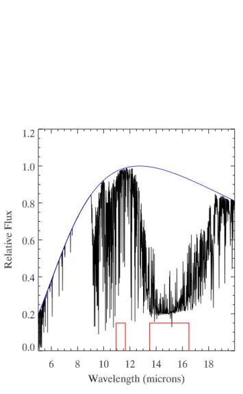
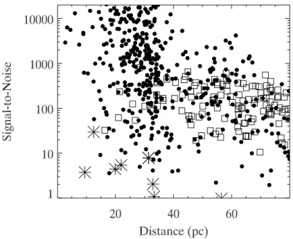
Figure 9 shows a model spectrum of a superEarth in the 5− to 20 µm spectral region, from Miller-Ricci et al. (2009), and marks the bandpasses of MIRI filters at 11.3− and 15 µm. Figure 10 shows the results of coupling the TESS simulations to our MIRI filter photometry noise model, for superEarths and exo-Neptunes. For superEarths we plot the SNR on the difference in contrast between the 11.3− and 15 µm bands, i.e., SNR on the absorption detection. For the exo-Neptunes, we plot the SNR in the 15 µm band alone, but the SNR for Neptunes is sufficiently high to contemplate much higher spectral resolution results as well. SNR will scale down from Figure 10 as the square-root of the number of eclipses. Neptune-sized planets will generally not require photometry of large numbers of eclipses in order to achieve good SNR. Figure 11 shows an example of simulated MIRI 15 µm photometry for 10 eclipses of a warm exoNeptune.
Eight habitable superEarths appear on Figure 10, but with lower SNR than for NIRSpec. This lower SNR arises in part from the background-limited nature of MIRI observations. The planet signal scales as the inverse square of the distance. However, as distance increases the noise approaches a constant level determined by the thermal background, hence SNR ∼ d−2
habitable superEarths attains higher SNR on average, because the NIRSpec SNR is predominately source-photon-limited and hence SNR ∼ d−1
, not ∼ d−2
. However, we expect the nearest habitable TESS superEarth to orbit a nearby (d. 10 pc) late-M dwarf, and MIRI will readily detect its secondary eclipse (Charbonneau & Deming 2007). We verified that the Charbonneau & Deming (2007) projections, as updated for their two cases by Charbonneau (2008), remain approximately consistent with our current MIRI noise model.
Many hotter superEarths are present on Figure 10 (filled circles), and their possible CO2 absorption can be characterized by JWST to SNR ∼ 10 or greater. Specifically,
there are 446 superEarths above SNR = 10 on Figure 10. Although our simulation adopts exactly one planet per star, only 40% of our planets are superEarths, close to the superEarth frequency claimed by Mayor et al. (2009). Adopting the Mayor et al. (2009) 30% frequency, TESS will discover ∼ 330 hot superEarths whose CO2 absorption can be
measured by MIRI filter photometry. Above the radius of superEarths (> 3R⊕ as defined
by TESS), TESS will find many Neptune-size planets (up to 5R⊕) whose eclipses can be
measured by MIRI to high SNR (Figure 11.)
6.2. NIRSpec Spectroscopy
We generate synthetic spectroscopy for a given synthetic planet by including the photon noise from the star, which can vary significantly with wavelength at the R = 1000 resolving power of NIRSpec, due to absorption features in the stellar spectra, especially for the M-dwarfs. We use Phoenix model spectra to represent the stars, and we adopt planet models from Miller-Ricci et al. (2009), as described in the MIRI case. Since we are here dealing with transmission spectra, we scale the magnitude of the absorption from the fiducial planet model(s) in proportion to the calculated scale height of each planets
atmosphere, and the circumference of its atmospheric annulus. The spectra of the fiducial models have been calculated in full detail on a line-by-line basis by Miller-Ricci et al. (2009). We preserve this spectrum shape, and scale the depth of the transmission spectrum in proportion to the projected area of the atmosphere. Note that the geometry of this problem causes an atmosphere to be opaque over a greater span in scale heights for larger planets. We include a radius-dependent factor to account for this effect. Our synthetic time-series spectroscopy includes fundamental fluctuations due to the uncorrectable portion of the intra-pixel effect, as described above. For this purpose we use a large collection of synthetic 10-sec exposures, and we draw a series of this nonGaussian noise starting at a random time for each transit of each planet.
Computation of the SNR for each wavelength in the transit spectrum proceeds by constructing multiple transit curves at each wavelength, including synthetic photon noise and intra-pixel fluctuations, and evaluating the SNR of the ensemble of transits, as described above for MIRI eclipses. The number of observable transits is taken to equal the number that can be observed for each planet by JWST during its 5-year mission, under the constraint of JWST’s field-of-regard. Having evaluated the SNR at each wavelength, we also calculate a total SNR for the entire band, via a quadrature summation of the SNR values at each wavelength: SNRband =p( P snri2), where the sum is over the number of wavelength
channels in the spectrum, and snri is the SNR at a single wavelength i, averaged over all
observed transits. When including the transmission signal in this calculation, we of course use only the variation in transmitted intensity vs. wavelength, not the total absorption due to the entire planet. Figure 12 shows the results of this calculation (SNRband) for water
absorption near 2 µm, and Figure 13 shows the corresponding result for detection of CO2
absorption at 4.3 µm.
superEarth, and Figure 15 shows examples of CO2 absorption in similar planets.
7. Discussion and Conclusions
7.1. Our Results
Using our default distribution that orbital sizes are distributed uniformly in log(a′
) (Sec. 3.1) places about 15% of our Monte-Carlo planets within the HZ of their star. Thus, from Figure 1 (interpolating between the 0.1 and 0.3 curve), we project that the nearest transiting habitable planet will lie about 10 parsecs distant from our Sun. The nearest transiting habitable planet produced by our simulation lies at 9.5 parsecs from our Sun. Hence our simulation is consistent with the calculation presented in Sec. 2. Moreover, as we show below, our sensitivity calculations are also internally consistent because our zeroth order results (Sec. 4) agree well with our more exhaustive calculations (Secs. 5 & 6). We therefore discuss the prospects for habitable superEarth discovery and characterization on the basis of our consistent, end-to-end simulation.
The above statements concerning nearby habitable planets are not restricted to superEarths, because our orbit distributions and radius distributions are independent. The architecture of our own solar system suggests that small planets should be associated with closer orbits, but we impose no such condition in our simulation. However, small planets outnumber large ones in our distributions, and the nearest transiting habitable planets we generate turn out to be superEarths, not Neptunes or Jupiters. Moreover, TESS finds these nearby habitable worlds very efficiently. Repeating our simulation 500 times, and considering only the superEarths, we tabulated the number of times that TESS finds at least one habitable superEarth closer than 35 pc. We adopted 0.3 superEarths per star (Mayor et al. 2009), with our default distribution in orbital radius. The Mayor et al.
(2009) estimate is a frequency: 30% of stars have at least one planet in the range up to Neptune-sized. The fact that Mayor et al. (2009) include Neptunes tends to make our 0.3 superEarths-per-star value too high, but the fact that many stars will have multiple planets works in the opposite direction. Thus we believe that our 0.3 superEarths-per-star value is reasonable, and it produces 0.047 superEarths per star in the habitable zone. With this abundance, TESS finds at least one transiting habitable superEarth closer than 35 parsecs in 495 out of 500 simulations, a 99% probability.
Nearby habitable transiting superEarths can be characterized to a significant degree by JWST. The level of significance for this characterization is a function of astrophysical uncertainties, not primarily technological ones. First, consider the situation for near-IR water absorption measured by transmission spectroscopy at transit. Our zeroth order calculation (Figure 4) indicates that water absorption could be measured in 5 nearby habitable superEarths to SNR equal or exceeding 10, versus 8 from Figure 12. A key difference in these figures is that Figure 4 adopts a 200-hour program, whereas Figure 12 is based on observing all transits available within the JWST mission lifetime. But habitable planets tend to have longer orbit periods (compared to ‘hot superEarths’), resulting in longer transits that occur less frequently. Inspecting the number of habitable superEarth transits available to JWST per system, we find a natural dividing point near 60 transits. Five of the eight Figure 12 habitable superEarths exhibit 60 or fewer transits, and the total in-transit time for each of them is less than 200 hours. These five habitable superEarths would be suitable to observe using a large JWST program. An example of synthetic JWST data for water absorption in a habitable superEarth with relatively low aggregate SNR (SNRband = 16) is shown in the lower panel of Figure 14. SuperEarths represent about 40%
of the planets in our simulation, close to the 30% frequency claimed by Mayor et al. (2009). (Hence, our simulations can be scaled to the Mayor et al. (2009) frequency by multiplying the number of superEarths by 0.75.) If their frequency is lower than Mayor et al. (2009)
claim, then the number available for JWST characterization will be reduced in proportion. Another source of astrophysical uncertainty regarding JWST characterization is the nature of the superEarth atmosphere. We have used the intermediate case of Miller-Ricci et al. (2009), where the atmosphere is mildly reducing and inflated in height by the presence of residual hydrogen (either primordial, or outgassed). In the absence of this hydrogen, the mean molecular weight increases, the scale height decreases, and the water abundance also decreases. In that case, the SNR for transmission spectroscopy drops by a factor of ∼ 3, but JWST characterization remains possible for the closest superEarths. Specifically, five habitable superEarths would remain above SNRband = 10, of which about
three could be observed in 60 or fewer transits. If the frequency of superEarths is as low as 0.1 per star, and their atmospheres are hydrogen-depleted, then the number capable of being characterized in water absorption by JWST is expected to be one. On the other hand, if the frequency estimate of Mayor et al. (2009) is correct, and also their atmospheres are mildly reducing (10% hydrogen), then the expectation for the number that JWST can characterize via water absorption is five.
The situation for detection of CO2 in absorption at 4.3 µm during transit is similar to
that of water. Figure 13 indicates seven habitable superEarths which could be observed to SNR ≧ 10, of which four can be observed in less than 60 transits. Synthetic data for one example is shown in the lower panel of Figure 15. This habitable superEarth has SNRband = 28, obtained by observing 58 transits. If the atmospheres of these worlds are
hydrogen-depleted, then the SNR drops by a factor of two, and the number remaining above SNR = 10 in 60 transits or less drops to two. Factoring in possible variation in superEarth frequency (as above), then our expectation for the number capable of being characterized in CO2 absorption by JWST to SNR = 10 ranges from one to five.
continuum radiation at secondary eclipse to SNR ≧ 10. Simulation of CO2 absorption
observations using MIRI photometry at 15 µm (Figure 10) indicate one superEarth having SNR ≧ 10, with an additional one at SNR = 8. These smaller numbers are consistent with the more demanding measurement of absorption vs. a simple continuum brightness temperature measurement. An additional 3 are present on Figure 10 with SNR ' 4, sufficient to establish at least the presence of CO2 absorption. Unlike the case of transit
spectroscopy, this secondary eclipse technique is not sensitive to the scale height of the atmosphere, only to the total column density of absorbing molecules. Therefore we need only consider the frequency of superEarths. On this basis we expect the number capable of being characterized via a thermal continuum temperature measurement, and identification of CO2 absorption is from one to four.
Although our projections as quoted above are from a single Monte-Carlo simulation of the TESS yield, we have re-run our simulations multiple times to verify the stability of the results in a statistical sense. We emphasize that JWST characterization of habitable worlds will require a large program, with priority given to the available transits/eclipses. Also, difficult choices will be necessary since each transit is precious but can be observed in only one mode (instrument, grating setting, etc.) at a time. Although the number of habitable planets capable of being characterized by JWST will be small, large numbers of warm-to hot-superEarths and exoNeptunes will be readily characterized by JWST, and their aggregate properties will shed considerable light on the nature of icy and rocky planets in the solar neighborhood.
7.2. Comparison to Other Results
Pioneering work by Valenti et al. (2006) considered the possibility of JWST/NIRSpec characterization of habitable terrestrial planets that may transit nearby M-dwarfs, based
on models by Ehrehreich et al. (1999). They find that a habitable ocean planet orbiting an M3V star at 13 parsecs distance (J-magnitude = 8) can be well characterized using NIRSpec transmission spectroscopy. However, they find that water and CO2 absorption in
an Earth-sized planet with a high molecular weight atmosphere, i.e., a true Earth analog, can be detected only if the planet orbits an unrealistically bright and nearby M-dwarf (J=5, lying at 3 parsecs distance). Our calculations specifically include realistic details such as the number of transits available within the JWST field-of-regard, effects of non-central transits, systematic errors in the instrument, etc. However, we find that inclusion of these realistic factors does not greatly degrade the JWST sensitivity, and we concur with the Valenti et al. (2006) results. Specifically, we note that none of the habitable planets above SNR = 10 on Figure 12 are true Earth analogs, but this does not diminish their importance. All of them have radii exceeding 1.8 R⊕, and most of them are ocean planets.
Recently, Kaltenegger & Traub (2009) have calculated the detectability of Earth’s transmission spectrum, illuminated by lower main sequence stars at 10 parsecs. They find that the transmission spectrum of our Earth has SNR < 1 for every molecular band in a single transit. However, many of the molecular features they tabulate would be observed to SNR > 10 in a 200-hour program (their Table 3).
Regardless of the situation for a true Earth analog, results for Earth cannot be easily extrapolated to superEarths. The atmospheric scale height is proportional to 1/g, where g is surface gravity. If we make the reasonable assumption that mass density is constant as radius varies, then g ∼ M/R2
p ∼ Rp. The projection of an atmospheric annulus of a given
scale height is then proportional to Rp/g, and thus absorption seems independent of Rp.
However, superEarths include ocean planets having lower mass densities (Seager et al. 2007; Fortney et al. 2007), which invalidates the assumption of constant density. Also, slant-path absorption does not scale strictly with H as Rp increases. In the slant-path geometry,
for a given line opacity (cm2
/g), the atmosphere is opaque over more scale heights as Rp
increases. This modest but significant factor is included in our calculations.
We reiterate our conclusion that, depending on the frequency of occurrence of superEarths and the nature of their atmospheres, JWST will be able to measure the temperature, and detect molecular absorption bands, in one to four habitable TESS superEarths.
T. Greene and M. Clampin gratefully acknowledge support from the JWST Project. We thank J. Valenti for sending us his exoPTF White Paper, and Lisa Kaltenegger for an advance copy of her ApJ paper. We are grateful to Tilak Hewagama for a clarifying discussion on simulation of JWST pointing jitter, and to the referee for helpful comments that significantly improved the manuscript.
REFERENCES Barnes, J. W., 2007, PASP, 119, 859.
Blake, C., Charbonneau, D., White, R. J., Marley, M., & Saumon, D. 2007, ApJ 666, 1198. Charbonneau, D., Brown, T. M., Noyes, R. W., & Gilliland, R. 2002, ApJ, 568, 377.
Charbonneau, D., Allen, L. E., Megeath, S. T., Torres, G., Alonso, R., Brown, T. M., Gilliland, R. L., Latham, D. W., Mandushev, G., O’Donovan, F., & Sozetti, A. 2005, ApJ 626, 523.
Charbonneau, D., and 10 co-authors, 2006, ApJ, 636, 445.
Charbonneau, D., Brown, T. M., Burrows, A., & Laughlin, G. 2007, Protostars and Planets V, p. 701.
Charbonneau, D., 2008, Opening review at IAU Symposium 253, Cambridge University Press, 253, 1.
Charbonneau, D., Knutson, H. A., Barman, T., Allen, L. E., Mayor, M., Megeath, S. T., Queloz, D., & Udry, S. 2008, ApJ, 686, 1341.
Charbonneau, D. & Deming, D. 2007, astro-ph/0706.1047. Clampin, M. 2008, SPIE, 7010, 70100L.
Clampin, M., JWST Transit Working Group, Deming, D., & Lindler, D. 2009, white paper submitted to the Astrophysics 2010 Decadal Survey.
Deming, D., Seager, S., Richardson, L. J., & Harrington, D. 2005, Nature 434, 740. Deming, D., Harrington, J., Seager, S., & Richardson, L. J. 2006, ApJ 644, 560.
Deming, D., Harrington, J., Laughlin, G., Seager, S., Navarro, S. B., Bowman, W. C., & Horning, K. 2007, ApJ, 667, L199.
Ehrenreich, D., Tinetti, G., Lecavelier des Estangs, A., Vidal-Madjar, A., & Selsis, F. 1999, A&A, 448, 379.
Forbrich, J., Lada, C. J., Muench, A. A., & Teixeira, P. S. 2008, ApJ, 687, 1107. Fortney, J. J., Marley, M. S., Barnes, J. W., 2007, ApJ, 659, 1661.
Gardner, J. P., et al. 2006, Space. Sci. Rev. 123, 485.
Greene, T., Beichman, C., Eisenstein, D., Horner, S., Kelly, D., Mao, Y., Meyer, M., Rieke, M., & Shi, F. 2007, Proc. SPIE, 6693, 66930G.
Gilliland, R. L., Nugent, P. E., & Phillips, M. M. 1999, ApJ, 521, 30.
Grillmair, C. J., Charbonneau, D., Burrows, A., Armus, L., Stauffer J., Meadows, V., van Cleve, J., & Levine, D. 2007, ApJ, 658, L115.
Grillmair, C. J., Burrows, A., Charbonneau, D., Armus, L., Stauffer, J., Meadows, V., van Cleve, J., von Braun, K., & Levine, D. 2008, Nature, 456, 757.
Hardya, T., Barilb, M. R., Pazdera, J., & Stilburna, J. S. 2008, SPIE, 7021, 70212B. Harrington, J., Hansen, B. M., Luszcz, S. H., Seager, S., Deming, D., Menou, K.,
Cho, J. Y.-K., & Richardson, L. J. 2006, Science, 314, 623.
Harrington, J., Luszcz, S., Seager, S., Richardson, J. L., & Deming, D. 2007, Nature 447, 691.
Hauschildt, P. H., Allard, F., Ferguson, J., Baron, E., & Alexander, D. R. 1999, ApJ, 525, 871.
Henry, T. J., Kirkpatrick, J. D., & Simons, D. A. 1994, AJ, 108, 1437. Kalas, P., et al. 2008, Science, 322, 1345.
Kaltenegger, L. & Traub, W. A. 2009, ApJ, in press (astro-ph/0903.3371). Kelsall, T., and 11 co-authors, 1998, ApJ, 508, 44.
Knutson, H. A., et al. 2007, Nature, 447, 183.
Knutson, H. A., Charbonneau, D., Allen, L. E., Burrows, A., & Megeath, S. T. 2008, ApJ, 673, 526.
Knutson, H. A., et al. 2009, ApJ, 690, 822.
Kohler, J., Melf, M., Posselt, W., Holota, W., & te Plate, M. 2005, Proc. SPIE, 5962, 563. Lunine, J. I., & 15 co-authors, 2008, Astrobiology, 8, 875.
Marois, C., Macintosh, B., Barman, T., Zuckerman, B., Song, I., Patience, J., Lafreniere, D., & Doyon, R. 2008, astro-ph/0811.2606
Mayor, M., & 9 co-authors, 2009, A&A, 493, 639.
Miller-Ricci, E., Sasselov, D. D., & Seager, S. 2008, ApJ, 690, 1056. Morales-Calderon, M., & 12 co-authors, 2006, ApJ, 653, 1454. Nutzman, P., & Charbonneau, D., 2008, PASP, 120, 317. Ostaszewski, M. & Vermeer, W. 2007, SPIE, 6665, 66650D. Rauscher, B. J., et al. 2007, PASP, 119, 768.
Reid, N., & Hawley, S. L., 2000, ‘New Light on Dark Stars: Red Dwarfs, Low-mass Stars, and Brown Dwarfs’, New York: Springer.
Redfield, S., Endl, M., Cochran, W. D., & Koesterke, L. 2008, ApJ, 673, L87.
Richardson, L. J., Deming, D., Horning, K., Seager, S., & Harrington, J. 2007, Nature, 445, 892.
Ricker, G. R., & 27 co-authors, 2008, AAS Meeting 213, 403.01. Seager, S. & Deming, D. 2009, submitted to ApJ.
Seager, S. & Sasselov, D. D. 2002, ApJ, 537, 916.
Seager, S., Kuchner, M., Hier-Majumder, C. A., & Militzner B. 2007, ApJ, 669, 2179. Seager, S., Deming, D., & Valenti, J. A. 2008, in ‘Astrophysics in the Next Decade: JWST
and Concurrent Facilities’, eds. H. A. Thronson, A. Tielens, & M. Stiavelli, Springer: Dordrecht (in press).
Swain, M. R., Vasisht, G., & Tinetti, G. 2008, Nature, 452, 329.
Swain, M. R., Vasisht, G., Tinetti, G., Bouwman, J., Chen, P., Yung, Y., Deming, D., & Deroo, P. 2009, ApJ, 690, L114.
Swinyard, B. M., Rieke, G., Ressler, M., Glasse, A., Wright, G., Ferlet, M., & Wells, M. 2004, Proc. SPIE, 5487, 785.
Tinetti, G., and 12 co-authors, 2007, Nature, 448, 169. Udry, S., & 10 co-authors, 2007, A&A 469, L43.
Valenti, J. A., and 15 co-authors, 2005, BAAS, 37, 1350.
Valenti, J. A., Turnbull, M., McCullough, P., & Gilliland, R. 2006, White Paper submitted to the Exoplanet Task Force.
Valenti, J. A., 2008, presentation at the JWST for Planetary Science Workshop, Ithaca NY, October, 2008.
Vidal-Madjar, A., Lecavelier des Etangs, A., D´esert, J.-M., Ballester, G. E., Ferlet, R., H´ebrard, G., & Mayor, M. 2003, Nature, 422, 143.
Winn, J. N., and 11 co-authors, 2008, ApJ, 683, 1076.
Wright, G. S., and 17 co-authors, 2004, Proc. SPIE, 5487, 653.
This manuscript was prepared with the AAS LA
Fig. 1.— Probability of a habitable transiting planet lying within a sphere of a given distance (radius) centered on the Sun, for planet frequencies of (left to right) 1.0, 0.3, and 0.1 per star, adopting the condition that all planets lie within the HZ (see text).
Fig. 2.— Number of planets detected by TESS in our simulations vs. radius, using two different distributions of planet orbital distance. The solid line is our default distribution, that places planets with uniform probability in log a, scaled by the stellar luminosity (see text). The dashed line places planets with uniform probability in a, between 0.05 and 1.0 AU.
Fig. 3.— Upper panel: Completeness of the TESS survey for the detection of transiting superEarths (1 − 3R⊕) orbiting main sequence stars of different masses, in a volume out to 35 parsecs distance. Lower panel: Completeness of the TESS survey for the detection of transiting superEarths orbiting in the habitable zone of stars of all spectral types, versus distance.
Fig. 4.— Upper panel: Contours of signal-to-noise ratio (SNR) for an intermediate com-position 10 M⊕ habitable superEarth (R = 2.3R⊕, T = 323K) observed during transit by
a large aperture space telescope (area 25 m2
), observing water absorption at 2 µm, using a spectral resolving power of 1000, and summing the SNR over the 160 most optically thick wavelengths. Lower panel: SNR contours for the secondary eclipse of the same habitable superEarth, observed in thermal continuum radiation using a large-aperture cryogenic space telescope at 15 µm, with a 3 µm optical bandwidth (FWHM). Both panels assume the av-erage of multiple transits or eclipses observed during a 200-hour program. The overplotted points show the TESS-discovered planets from our simulation, choosing all planets having radii R = 2.3 ± 1.0 R⊕, and T = 323 ± 50 K.
Fig. 5.— Like Figure 3, but using a planet of 20 M⊕, R = 2.7R⊕, hydrogen-helium-dominated
atmospheric composition, and T = 500K. The overplotted points are all TESS-discovered planets from our simulation, having R = 2.7 ± 1.0 R⊕, and T = 500 ± 50 K.