Trace-zero subgroups of elliptic and twisted Edwards curves : a study for cryptographic applications

(1)

Trace-zero subgroups

of elliptic and twisted Edwards curves:

a study for cryptographic applications

TH`

ESE DE DOCTORAT

Candidat :

Giulia Bianco

Directrice de th`ese:

Prof. Elisa Gorla, Universit´e de Neuchˆatel

Rapporteurs:

Dr. Peter Birkner, Federal Office for Information Security (BSI) Dr. Hugues Mercier, Universit´e de Neuchˆatel

Ann´ee Acad´emique 2016-2017

Institut de Mathématiques, Université de Neuchâtel Rue Emile-Argand 11, CH-2000 Neuchâtel (Suisse)

(2)

(3)

Imprimatur pour thèse de doctorat www.unine.ch/sciences

Faculté des Sciences

Secrétariat-décanat de Faculté Rue Emile-Argand 11 2000 Neuchâtel – Suisse Tél : + 41 (0)32 718 21 00 E-mail : secretariat.sciences@unine.ch

IMPRIMATUR POUR THESE DE DOCTORAT

La Faculté des sciences de l'Université de Neuchâtel

autorise l'impression de la présente thèse soutenue par

Madame Giulia BIANCO

Titre:

“Trace-Zero subgroups of elliptic and twisted

Edwards curves: a study

for cryptographic applications”

sur le rapport des membres du jury composé comme suit:

! Prof. Elisa Gorla, directrice de thèse, Université de Neuchâtel, Suisse

! Dr Hugues Mercier, Université de Neuchâtel, Suisse

! Dr Peter Birkner, Federal Office of information security, BSI, Bonn, Allemagne

(4)

(5)

(6)

(7)

Clever talk alarmed her, and withered her delicate imaginings; it was the social counterpart of a motor-car, all jerks, and she was a wisp of hay, a flower.

E. M. Forster, Howards End

C’era una volta una ragazzina che, quando doveva risolvere un problema, diventava ansiosa, e allora chiedeva aiuto alla “ Regina degli animali ”. Al suo richiamo lupi e balene accorrevano con il loro flusso magico. Ma non era necessario il loro intervento perch´e la ragazzina era molto brava.

La ragazzina adesso è una giovane donna. Un ultimo esame da superare per terminare il suo brillante dottorato. “ Regina degli animali, mi serve aiuto da lupi e balene ” Seduta sugli scogli la Regina lancia il suo richiamo: “ Balene, la mia principessa ha bisogno di voi ! ” Poi chiama il suo amico Eolo e si fa trasportare nella foresta, lanciando il suo richiamo ai lupi. Tutti rispondono alla sua richiesta di aiuto. “ Ma in tutti questi anni il nostro flusso magnetico non è servito a niente” ( dice il vecchio lupo e la balena acconsente ) “ La principessa è bravissima. Questa è l’ultima volta che veniamo da lei!!” Non possiamo perdere tempo con ci chiama solo perché è in ansia . Addio principessa, puoi benissimo affrontare da sola la tua vita!. Nonna Adriana

(8)

(9)

Summary

In 1999, Frey first suggested trace-zero subgroups of elliptic curves for applications to cryp-tography, as a valid alternative to the use of classical groups of points of elliptic curves in this sector. Take an elliptic curve E defined over a finite field Fq, with the standard

addition between points. Given a field extension Fq ⊆ Fqn of odd prime degree n, the

trace-zero subgroup of the elliptic curve E of degree n is a subgroup of the group of points of E with coordinates in Fqn.

In 2007, Edwards curves were introduced by Edwards, and proposed for cryptographic applications by Bernstein and Lange. Right afterwards, they were generalized to twisted Edwards curves. Twisted Edwards curves can be seen as special elliptic curves, written in a new form. They have some cryptographic advantages over elliptic curves in the usual Weierstrass form. Trace-zero subgroups of twisted Edwards curves are defined in the same way as trace-zero subgroups of elliptic curves.

In this thesis, we study trace-zero subgroups of elliptic and twisted Edwards curves, from the point of view of their potential application to cryptography. In particular, we focus on three distinct aspects for trace-zero subgroups: the use of optimal representations for group elements, the construction of fast algorithms for scalar multiplication, and the study of possible cryptographic attacks based on the discrete logarithm problem. All these aspects are of great relevance for the efficiency and the security of a cryptosystem built on the given group.

Concerning optimal representations for group elements, we propose two optimal repre-sentations for trace-zero subgroups of twisted Edwards curves. We give efficient algorithms to deal with them, and we make comparisons with analogous representations for trace-zero subgroups of elliptic curves.

Concerning efficient arithmetic in trace-zero subgroups, our contribution consists of an algorithm to perform scalar multiplication in the trace-zero subgroup of degree three. This algorithm follows an original approach and makes use of optimal coordinates to represent the elements of the group.

Finally, we focus on the study of security of trace-zero subgroups against cryptographic attacks. We propose a new variant of the index calculus algorithm for the discrete loga-rithm problem in these subgroups. We compare the complexity of solving the polynomial systems obtained with our method with that of solving the systems computed with the only other specialization of the index calculus to trace-zero subgroups. We show that our systems are easier to solve in the case of trace-zero subgroups of small degree, that is the important case for cryptographic applications.

(10)

In both the algorithm for scalar multiplication in trace-zero subgroups of degree three, and in our new index calculus method for trace-zero subgroups, we make use of generalized summation polynomials of elliptic curves. Such polynomials are introduced in this thesis for the first time, and they can be seen as an original generalization of Semaev’s summation polynomials of elliptic curves. Generalized summation polynomials allow to find relations between points on the elliptic curve. Thanks to their geometric property, they can have relevant applications to cryptography.

Keywords. Cryptography, elliptic curves, twisted Edwards curves, optimal represen-tations for group elements, compression and decompression, Semaev’s summation poly-nomials, generalized summation polypoly-nomials, efficient scalar product, discrete logarithm problem, index calculus.

(11)

Resum´

e

En 1999, Frey a proposé, pour la première fois, les sous-groupes de trace nulle des courbes elliptiques pour les applications à la cryptographie: il les a désignés comme une alternative valide, dans ce secteur, aux groupes classiques des points des courbes elliptiques. Con-sidérons une courbe elliptique E définie sur un corps fini Fq, avec l’addition standard entre

ses points. Etant donn´ee une extension de corps Fq ⊆ Fqn de degr´e n premier et impair,

le sous groupe de trace nulle de la courbe elliptique E, de degr´e n, est un sous-groupe du groupe des points de E avec coordonn´ees dans Fqn.

En 2007, les courbes d’Edwards ont été introduites par Edwards, et elles ont été pro-posées pour les applications cryptographiques par Bernstein et Lange. Après, elles ont été généralisées aux courbes d’Edwards tordues. Les courbes d’Edwards tordues peuvent être considérées comme des courbes elliptiques speciales, éctrites sous une nouvelle forme. Elles ont des advantages cryptographiques sur les courbes elliptiques dans la forme usuelle de Weierstrass. Les sous-groupes de trace nulle des courbes d’Edwards tordues sont definies de la même manière que les sous-groupes de trace nulle des courbes elliptiques.

Dans cette thèse, nous étudions les sous-groupes de trace nulle des courbes elliptiques et des courbes d’Edwards tordues, du point de vue de leur application potentielle à la cryptographie. En particulier, nous nous concentrons sur trois aspects distincts pour les sous-groupes de trace nulle: l’utilisation de représentations optimales des éléments du groupe, la construction d’algorithmes pour le produit scalaire, et l’étude de possibles at-taques cryptographiques basés sur le problème du logarithme discret. Tous ces aspects sont tres importants pour l’efficacité et la sécurité d’un cryptosystème construit sur le groupe considéré.

`

A propos de représentations optimales de groupes, nous proposons deux représentations optimales pour les sous-groupes de trace nulle des courbes d’Edwards tordues. Nous don-nons des algorithmes efficaces pour l’utilisasion de nos représentations, et nous faisons des comparaisons avec les représentations analogues pour les sous-groupes de trace nulle des curbes elliptiques.

En ce qui concerne l’arithmétique efficace dans les sous-groupes de trace nulle, notre contribution consiste en un algorithme pour effectuer le produit scalaire dans les sous-groupes de trace nulle de degré trois. Cet algorithme suit une approche originale et il utilise des coordonnées optimales pour représenter les éléments du groupe.

Enfin, nous nous concentrons sur la sécurité des sous-groupes de trace nulle contre les attaques cryptographiques. Nous présentons une nouvelle variante de l’algorithme d’index calculus pour le problème du logarithme discret dans ces sous-groupes. Nous comparons

(12)

la complexité de la résolution des systèmes polynômiaux obtenus avec notre méthode à celle de la résolution des systèmes construits avec l’unique autre spécialisation d’index cal-culus aux sous-groupes de trace nulle. Nous montrons que nos systèmes sont plus faciles `

a r´esoudre, dans les cas de sous-groupes de trace nulle de degr´e petit, qui sont les cas importantes pour les applications cryptographiques.

Dans l’algorithme pour le produit scalaire dans les sous-groupes de trace nulle de degré trois, et dans notre nouvelle méthode d’index calculus, nous utilisons les polynômes de sommation généralisés de courbes elliptiques. Ces polynômes sont présentés dans cette thèse pour la première fois, et ils peuvent être vus comme une généralisation originale des polynômes de sommation de courbes elliptiques de Semaev. Les polynômes de sommation généralisés permettent de trouver des relations entre points sur la courbe elliptique. Grâce `

a leur propriété géométrique, ils peuvent avoir des applications pertinentes en cryptogra-phie.

Mots clés. Cryptographie, courbes elliptiques, courbes d’Edwards tordues, représentations optimales de groupes, compression et décompression, polynômes de sommation de Semaev, polynômes de sommation généralisés, produit scalaire efficace, problème du logarithme discret, index calculus.

(13)

List of Symbols and Notation

Z The integers. p. 2

Z>n The integers bigger than n ∈ Z . p. 2

Z≥n The integers bigger or equal than n ∈ Z . p. 2

ZN The integers modulo N , N ∈ Z>1. p. 4

Fq A finite field with q elements (q prime power). p. 6

hP i Cyclic group generated by P . p. 2

DLP Discrete Logarithm Problem. p. 3

log_P(Q) Discrete logarithm of Q ∈ hP i w.r.t. P . p. 3

O(), o() Big-O notation, small-o notation. p. 3

Ω() Big-Ω notation. p. 3

LN(α, c) exp ((c + o(1))(log N )α(log log N )1−α), p. 3

0 ≤ α ≤ 1, c > 0.

R = (RG)G∈G Optimal representation for G, p. 5

G family of finite groups.

K, K, K ⊆ L ⊆ K A field, its algebraic closure, a field extension. p. 7

K[x1, · · · , xn] The ring of polynomials with coefficients in K p. 30

and n ∈ Z≥1 variables xi.

K[x, y], K[x, y, z] Ring of polynomials with coefficients in K pp. 7, 8 and variables x, y (resp. x, y, z).

deg (f ) Total degree of f ∈ K[x1, · · · , xn]. p. 7

(14)

deg_x_if _{Degree of f ∈ K[x}1, · · · , xn] in xi. p. 89

fh(x1, · · · , xn, xn+1) Homogenization of f (x1, · · · , xn) w.r.t. xn+1. p. 9

I = (f1, · · · , fs) Ideal generated by fi∈ K[x1, · · · , xn]. p. 124

Ih Homogeneous ideal Ih_{= (f}h

1, · · · , fsh). p. 125

A2(K), A2 Affine plane over K. p. 7

P2(K), P2 Projective plane over K. p. 8

An(K), An Affine space of dimension n over K, n ∈ Z≥2 p. 30

Pn(K), Pn Projective space of dimension n over K, n ∈ Z≥2 p. 30

Ca: f (x, y) = 0 Affine plane curve defined by p. 7

the polynomial f (x, y) ∈ K[x, y].

C: F (x, y, z) = 0 Projective plane curve defined by p. 8 F(x, y, z) ∈ K[x, y, z].

Ca(L), C(L) L-rational points of Ca (resp. C). pp. 7, 8

Ca Projective closure of Ca. p. 9

C_x∗, C_y∗, C_z∗ Affine dehomogenization of C w.r.t. x, y or z. p. 9

L[Ca] L-coordinate ring of Ca. p. 10

L(Ca), L(C) L-rational functions of Ca, C. pp. 10, 11

O_P(C) Local ring of C : f (x, y) = 0 at P , p. 13 C absolutely irreducible affine curve.

MP(C) Maximal ideal of OP(C). p. 13

ordP Order function of OP(C), p. 13

P nonsingular point of C.

Div(X) Group of divisors of X absolutely irreducible, p. 15 nonsingular projective curve.

div(r) Divisor of r rational function of X. p. 15

Div0(X) Group of divisors of X of degree 0. p. 15

(15)

xv

Pic0(X) Degree zero Picard group of X. p. 15

Pic0(X)(L) Group of L-rational divisor classes of X. p. 15

L(D) Vector space associated to D ∈ Div(X). p. 16

`(D) Dimension of L(D). p. 16

g Genus of an absolutely irreducible p. 16 projective curve.

EW Elliptic curve in Weierstrass form. p. 19

EM Elliptic curve in Montgomery form. p. 20

P_∞ Point at infinity of an elliptic curve. p. 20

Ea,d Twisted Edwards curve p. 24

with parameters a, d.

Ω1, Ω2 The two points at infinity of Ea,d. p. 24

E Elliptic curve, or E = (Ea,d)∗z. p. 20, 25

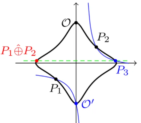
⊕ Point addition on elliptic curves pp. 20, 27 or on twisted Edwards curves.

−P Inverse of a point P w.r.t. ⊕. pp. 20, 25

O Neutral element of ⊕. p. 27

ϕ Frobenius endomorphism of E. p. 22

χϕ Characteristic polynomial of ϕ. p. 22

fn(x1, · · · , xn) The n-th summation polynomial of EW. p. 27

fn(y1, · · · , yn) The n-th summation polynomial of Ea,d. p. 27

Va Affine algebraic set. p. 30

Vp Projective algebraic set. p. 30

Va Projective closure of Va. p. 30

(16)

L(Va) L-rational functions of Va affine variety. p. 30

L(Vp) L-rational functions of Vp projective variety. p. 30

V Abelian variety. p. 31

dim(Va), dim(Vp), dim(V ) Dimension of a variety. p. 31

WE Abelian variety obtained from E(Fqn) p. 32

via Weil restriction of scalars.

Tr Trace endomorphism of E(Fqn). p. 33

Tn Trace-zero subgroup of E(Fqn). p. 33

T_n Trace-zero variety. p. 33

St,n1,··· ,nt A (t, n1, · · · , nt)-generalized p. 78

summation polynomial, t, ni ∈ Z≥2.

F A factor base for the index calculus. p. 40

DRL ordering The degree-reverse-lexicographic p. 124 monomial ordering.

D= solv.deg(I) Solving degree of I = (f1, · · · , fs) p. 124

w.r.t. the DRL ordering.

MD Macaulay matrix of the polynomial p. 124

(17)

Acknowledgements

Thank you to my supervisor, Elisa Gorla.

Thank you Elisa for the enthusiasm you put into your job, and the energy that spreads around you. For your constructive criticism, that makes me learn so much. For the time you have always dedicated to me, even when you had a million of other things to do and to care about.

To little Marina, for making us all happy.

To Alberto, my historical office-mate.

Grazie di tutto Albertoso. Sei un fratello maggiore per me.

To Alessio and his super wife Elisa, i miei cari amici neuchatellosi barcellonesi genovesi.

To Relinde, for her useful suggestions about this thesis, and for all lunches together.

To Roberta, because she knows my favorite biscuits.

To Anurag, for the fundamental yellow paper where I wrote all the thesis.

Thank you to my family, with all my love. Grazie alla mia famiglia, con tutto il mio cuore.

Alla mia Mamma Silvia.

Al mio Pap`a Sergione.

Grazie Mamma e Pap`a.

A mio fratello Francesco, la nostra ancora di salvezza e il nostro piccolo sciamano.

Alle mie Nonne carissime. Alla Nonna Adriana e alla Nonna Rosa.

Al mio Nonno Sandro che guarda dal cielo la sua Julie. Nonno, questa tesi `e dedicata a te.

A Stefano e a Jasmin. To my uncle Sandro.

Thank you to all my dear friends.

(18)

Alle ragazze dell’Asse, che ci sono sempre. Anna, Chiara, Elisa, Sara.

A Sara e Nico.

Alla mia amica giramondo Shanti.

Thank you to Matteo.

(19)

Introduction

In this thesis we study trace-zero subgroups of elliptic and twisted Edwards curves, from the point of view of their potential application to cryptography. In fact, such groups can be a valid alternative to the standard use of elliptic curves in this area.

Cryptography is the study of techniques that guarantee secret communication between parties. Nowadays, it is of crucial importance for all computer security, from safe elec-tronic commerce to trusted web authentication via a password.

In the basic cryptographic scenario, two people need to communicate, without being un-derstood by malicious third parties. Hence, they encrypt and decrypt their messages with the use of secret keys. Messages and keys are, in important real cryptosystems, elements of a cyclic group G of prime order. This group has to ensure efficient and safe communi-cation at the same time. From the point of view of efficiency, it is necessary to know fast algorithms to perform the arithmetic in G. Moreover, we need to represent group elements with the least possible number of bits, in order to save storage space. From the point of view of security, we need that the Discrete Logarithm Problem (DLP) in the group G is difficult to solve.

Among the groups that satisfy the efficiency and security conditions mentioned above, the groups of points of elliptic curves play an important role. Such groups are nowadays widely used in cryptographic applications. They are the first example of how algebraic geometry can be applied to cryptography.

Nevertheless, it is possible to go beyond this first example, as Frey suggested in [43]. In his paper, Frey proposed to get a deeper insight in the geometric world, in order to find valid alternatives to standard elliptic groups for the cryptographic setting. This was the first time that trace-zero subgroups of elliptic curves were proposed for applications to cryptography.

Let E be an elliptic curve defined over a prime field Fq, the so-called base field of E.

We denote by ⊕ the standard point addition on E, whose neutral element O is the point at infinity of the curve. For each field extension Fq ⊆ L, we denote by (E(L), ⊕) the abelian

group of L-rational points of E, which consists of all affine points of E with coordinates in L and the point at infinity. Moreover, we denote by ϕ the Frobenius endomorphism of the curve E, that raises each coordinate of a point of E to the q-th power.

For n an odd prime and the degree n field extension Fq ⊆ Fqn, we define the trace-zero

subgroup Tn ⊆ E(Fqn) as the group of points P ∈ E(F_qn) such that the sum of the n

Frobenius conjugates of P is zero:

Tn= {P ∈ E(Fqn) : P ⊕ ϕ(P ) ⊕ · · · ⊕ ϕn−1(P ) = O}.

It turns out that trace-zero subgroups satisfy the security and efficiency conditions to set up a safe cryptosystem. Regarding security, it can be shown that the security of

(20)

degree three trace-zero subgroups against DLP attacks is comparable to the security of groups of base field-rational points of elliptic curves, of the same size. These latter groups achieve the optimal security against such kind of attacks. This means that the best known algorithm to solve the DLP in them is the Pollard’s rho method, which works in any group independently of its specific structure. On the other hand, in trace-zero subgroups Tn one

can apply the index calculus algorithm for abelian varieties proposed by Gaudry in [46]. The complexity of this algorithm is the same as Pollard’s rho complexity for n = 3. Therefore, the degree 3 trace-zero subgroup achieves the optimal security against DLP attacks. For n ≥ 5, Gaudry’s strategy lowers in theory the complexity of solving the DLP. However, the method requires solving huge polynomial systems, and this task is often infeasible in practice, even for small n.

Again from the point of view of security, it can be shown that solving a DLP in E(Fqn)

is the same as solving a DLP in E(Fq) and a DLP in Tn. Hence, the increase in the security

level from the group E(Fq) to the group E(Fqn) is the same as the increase from E(F_q)

to the subgroup Tn. This means that, instead of working in the whole group E(Fqn), we

can restrict ourselves to the subgroup Tn, without loosing security. This is an advantage

if we use an optimal representation for trace-zero elements.

In this case, to use an optimal representation for group elements means to associate to each element of the group the shortest possible tuple of coordinates of Fq. Each coordinate

of Fqcan be easily translated in a bit-string via its binary representation. Therefore, points

of the group will be treated in a computer as bit-strings of the shortest possible length. As a consequence, they will be stored in the minimal space. It can be shown that the cardinality of E(Fqn) is about qn, while the cardinality of T_n is about qn−1. Therefore,

elements of the whole group E(Fqn) are optimally represented via n coordinates of F_q. On

the other hand, only n−1 coordinates of Fqare required to optimally represent elements of

the trace-zero subgroup. Hence, using an optimal representation for trace-zero elements, one can enjoy the benefit of optimal data storage for the level of security. In fact, various optimal representations are known for trace-zero subgroups of elliptic curves: see for example [62] for n = 3, [75] for n = 5, [27] and [69] for n = 3, 5, [47],[49].

Optimal representations for trace-zero elements can only be a practical advantage in the cryptographic setting if they are integrated with efficient algorithms to perform the arithmetic of the group. In this way, the benefit of saving storage space goes together with the efficiency of the computation in the group. One possible approach to this issue is to recover trace-zero elements from their optimal representations, then perform the efficient standard arithmetic in E(Fqn) and, in the end, compute the optimal representation of the

result. This method requires fast algorithms for compression and decompression: com-pression is the process of computing the optimal representation of a point, decomcom-pression is the inverse procedure. In fact, all previously cited works about optimal representations of trace-zero elements give efficient compression and decompression algorithms. It follows that the combination of optimal data storage for security level and efficient arithmetic is made effective in the cryptographic scenario. Moreover, in the trace-zero subgroup, we can exploit the properties of the Frobenius endomorphism of the elliptic curve in this subgroup, in order to speed up the computation of the standard scalar multiplication of points: see [6, Section 15.3], [4], [55], [62], [75]. We remark that, for important cryp-tographic applications like the Diffie-Hellman key exchange, scalar multiplication is the primary operation to be taken into account. Using the mentioned technique based on the Frobenius endomorphism, one has that scalar multiplication in Tn is faster than in the

whole group E(Fqn). Furthermore, it has been empirically verified that, thanks to the

(21)

xxi

in classical groups of base field-rational points of elliptic curves, of the same size (see [5]). We conclude that trace-zero subgroups provide a suitable combination of all security and efficiency aspects that are required for cryptographic applications, and that they can be a real, valid alternative to the standard use of elliptic curves.

Twisted Edwards curves are a quite recent development in cryptography. Edwards curves were first introduced by Edwards in 2007 ([34]). Right afterwards, they were proposed for cryptographic applications by Bernstein and Lange ([13]). They were then generalized to twisted Edwards curves ([12]). It can be shown that each twisted Edwards curve can be turned into an elliptic curve, by performing a rational change of variables. Therefore, we can see twisted Edwards curves as special elliptic curves, written in a new form. It follows that one can define addition of points of a twisted Edwards curve. More-over, groups of points of twisted Edwards curves can be used in cryptography in the same way as groups of points of elliptic curves. Furthermore, groups of points of twisted Ed-wards curves have some security and efficiency advantages over the standard groups of points of elliptic curves. In fact, it can be shown that their arithmetic is faster (see [13], [14], [11][12], [19]), and that they are safer against certain types of cryptographic attacks (see [13], [12]).

Trace-zero subgroups of twisted Edwards curves are defined in the same way as trace-zero subgroups of elliptic curves. They have all the good cryptographic properties of trace-zero subgroups of elliptic curves mentioned before.

The thesis is organized as follows. Chapter 1 contains preliminary definitions and results, that are useful to understand the further work. In Chapter 2, we propose two optimal representations for trace-zero subgroups of twisted Edwards curves, with efficient compression and decompression algorithms. In Chapter 3, we introduce generalized sum-mation polynomials, which will be used in the subsequent chapters. In Chapter 4, we give a new algorithm to perform scalar multiplication in the degree three trace-zero subgroup. Finally, Chapter 5 deals with a specialization of the index calculus algorithm proposed by Gaudry in [46] to trace-zero subgroups.

Chapter 1 is divided into five sections. Section 1.1 is a brief introduction to cryptog-raphy. It allows to understand how the work presented in the thesis can be of practical interest in this sector. In Section 1.2, we give basic notions about affine and projective curves. This notions will be used throughout the thesis to deal with the objects that we study, and to prove our results. In Section 1.3, we introduce elliptic curves and twisted Edwards curves, underlying their role in cryptography. Section 1.4 contains a detailed presentation of the main objects of the thesis, that are trace-zero subgroups of elliptic and twisted Edwards curves. In this survey, we point out and explain the main aspects that make trace-zero subgroups remarkable from the cryptographic point of view. In Section 1.5, we speak about the discrete logarithm problem in groups, whose hardness is funda-mental for the security of cryptosystems. We focus on the strategy of index calculus for the solution of the DLP, and on the version of this algorithm proposed by Gaudry in [46], which can be applied to trace-zero subgroups.

In Chapter 2, we propose two optimal representations for trace-zero subgroups of twisted Edwards curves, giving efficient compression and decompression algorithms for both of them. The motivation of this study is the importance to combine the benefit of optimal data storage with an efficient performance of the arithmetic of the group. More-over, as we pointed out before, twisted Edwards curves have been recently introduced in

(22)

cryptography, and they have some advantages over standard elliptic curves. Furthermore, all the previously cited works, about optimal representations for trace-zero subgroups, take trace-zero subgroups of elliptic curves. Therefore, to the extent of our knowledge, these are the first optimal representations to be proposed for trace-zero subgroups of twisted Edwards curves. Our representations, with annexed algorithms, are non-straightforward adaptations of the representations proposed in [47] and [49] for trace-zero subgroups of elliptic curves.

In Chapter 3, we introduce generalized summation polynomials of elliptic curves, and give a recursive algorithm to construct them. These polynomials allow to find relations be-tween points of the curve. They can be seen as a generalization of summation polynomials of elliptic curves, introduced by Semaev in [67]. Thanks to their geometric property, gen-eralized summation polynomials can have relevant applications to cryptography. In fact, we use them in both Chapter 4 and Chapter 5. Chapter 4 contains a constructive crypto-graphic application of generalized summation polynomials to cryptography, that provides an efficient algorithm to perform scalar multiplication in the degree three trace-zero sub-group. On the other hand, Chapter 5 describes a destructive cryptographic application of these polynomials, to the study of a new index calculus strategy for DLP attacks in trace-zero subgroups.

In Chapter 4, we give an algorithm to perform scalar multiplication in the degree three trace-zero subgroup of an elliptic curve, using the optimal coordinates proposed in [49] to represent the elements of the group. The motivation of this work is again to integrate the use of an optimal representation for trace-zero elements with efficient performances of the arithmetic in the group. We pointed out that a possible approach to this task is to decompress the trace-zero point that we want to multiply, to perform the standard scalar multiplication of points on elliptic curves, and then to compress the obtained result. On the other hand, the algorithm that we propose in this chapter follows the alternative ap-proach. Namely, it performs scalar multiplication in the degree three trace-zero subgroup, using directly the optimal coordinates of the given representation, without decompression and compression of points. To the extent of our knowledge, it is the first algorithm that performs the scalar product in the trace-zero subgroup with the direct approach in optimal coordinates.

Furthermore, our algorithm adapts the technique that makes use of the Frobenius endo-morphism of the elliptic curve, to speed up the standard scalar multiplication of points of the trace-zero subgroup. Therefore, we maintain the advantages of this strategy, even performing the operation directly in the optimal coordinates.

In Chapter 5, we propose a new variant of index calculus for trace-zero subgroups of elliptic curves. Our algorithm is a specialization, to trace-zero subgroups, of the index calculus algorithm proposed by Gaudry in [46]. To the extent of our knowledge, the only other specialization of this algorithm to trace-zero subgroups is given in [48]. As we mentioned before, the bottleneck of Gaudry’s strategy is that one has to deal with huge polynomial systems, and the computation of their solutions is often not feasible in practice. Therefore, the goal of our work was to construct new polynomial systems, in alternative to those proposed in [48], that are easier to solve in the case of small n, that is the important case for cryptographic applications. We succeed in our aim, and prove that the complexity of solving our polynomial systems is in most cases lower than the complexity of solving the systems of [48], in the cryptographic relevant cases of n = 3, 5, 7.

(23)

xxiii

In the Appendix, we list the explicit formulas and equations that we found, using some of the procedures and algorithms given in the thesis. We used these formulas and equations to make computations, examples and practical experiments.

We performed explicit computations and implemented algorithms with Magma ([22], [23]), version V2.22-1 of the software, running on a single 3 GHz core.

Articles

The new results in this thesis are contained in the following articles.

1. G. Bianco, E. Gorla, Compression for trace zero points on twisted Edwards curves, Journal of Mathematical Cryptology 10, no. 1 (2016), 15-34.

2. G. Bianco, E. Gorla, Scalar multiplication in compressed coordinates in the trace-zero subgroup, submitted (2017), available at https://arxiv.org/abs/1709.04178.

3. G. Bianco, E. Gorla, Index calculus in trace-zero subgroups and generalized summa-tion polynomials, preprint (2017).

The results of Chapter 2 are contained in 1. The results of Chapter 3 and 5 are contained in 3. The results of Chapter 4 are contained in 2.

(24)

(25)

1.1 Introduction to cryptography . . . 1 1.1.1 Security and efficiency issues to set up a good cryptosystem . . . 2 1.2 Affine and projective curves . . . 7 1.2.1 Rational functions and rational maps . . . 9 1.2.2 Local rings and singular points . . . 12 1.2.3 Divisors and genus . . . 14 1.3 Elliptic and twisted Edwards curves in cryptography . . . 17 1.3.1 Elliptic curves . . . 18 1.3.2 Twisted Edwards curves . . . 22 1.3.3 Summation polynomials of elliptic and twisted Edwards curves . . . 26 1.4 Trace-zero subgroups . . . 28 1.4.1 Beyond elliptic curve cryptography: admissible abelian varieties . . . 28 1.4.2 Trace-zero subgroups for cryptography . . . 31 1.5 Index calculus for the discrete logarithm problem . . . 36 1.5.1 Generic algorithms for the DLP . . . 36 1.5.2 Better than generic: exploit the structure to attack the cryptosystem 37 1.5.3 Index calculus . . . 38

2 Optimal representations 43

2.1 An optimal representation using summation polynomials . . . 45 2.1.1 Explicit equations, complexity, and timings for n = 3 . . . 51 2.1.2 Explicit equations, complexity, and timings for n = 5 . . . 55 2.2 An optimal representation using rational functions . . . 58 2.2.1 Explicit equations, complexity, and timings for n = 3 . . . 65 2.2.2 Explicit equations, complexity, and timings for n = 5 . . . 68

(26)

3 Generalized summation polynomials 71 3.1 A generalization of Semaev’s summation polynomials . . . 71 3.2 Definition of generalized summation polynomials . . . 73 3.3 Computation of generalized summation polynomials . . . 75 3.4 Degree of generalized summation polynomials . . . 84 3.5 Generalized summation polynomials for cryptography . . . 86

4 Scalar product in T3 87

4.1 Preliminaries, notations and formulas . . . 88 4.2 Scalar multiplication in T3 in compressed coordinates . . . 96

4.2.1 Subalgorithm and special cases . . . 96 4.2.2 A first algorithm for scalar multiplication . . . 101 4.2.3 The optimized algorithm for scalar multiplication . . . 104 5 Index calculus in trace-zero subgroups 109 5.1 Index calculus for trace-zero subgroups . . . 110 5.1.1 Computation of the polynomial system . . . 112 5.1.2 Polynomial systems for n = 3 . . . 114 5.2 Complexity of the polynomial systems . . . 115 5.2.1 Solving degree and maximal Macaulay matrix for the system . . . . 116 5.2.2 Experiments and timings for n=3 . . . 118 5.3 A hybrid approach for n = 5 . . . 119 5.3.1 Construction of the polynomial system . . . 120 5.3.2 Experiments, timings and comparisons . . . 122

Conclusions 125

A Explicit formulas 133

A.1 Computation of a (2, 3, 3)-generalized summation polynomial . . . 133 A.2 Doubling and tripling formulas in T3 . . . 134

A.2.1 Doubling formulas . . . 134 A.2.2 Tripling formulas . . . 135 A.3 Polynomial systems for index calculus in T3 . . . 135

(27)

Chapter 1

Preliminaries

1.1 Introduction to cryptography

WhatsApp Messenger is one of the most popular smartphone application for text messages and phone calls. It enables the client to use his phone number as well as the internet to send text messages and make voice and video calls for free. It was created in 2009 by J. Koum. Since February 2016, it has more than one billion users. In 2012, the WhatsApp company started introducing encryption in its systems, to ensure secure communication between the users. The encryption process of all WhatsApp structures was officially completed in April 2016.

WhatsApp is a bright example of the massive presence of cryptography in our everyday life. This is the reason why we choose it to start our little excursus on this topic. We now give a general idea of how WhatsApp encryption works. We exploit such a real scenario to collect and recall fundamental definitions, problems and tools of modern cryptography. These notions establish the basis and the motivations of the thesis.

General informations about WhatsApp can be found at https://www.whatsapp.com and https://en.wikipedia.org/wiki/WhatsApp. As regards the technical aspects of What-sApp encryption, we refer to [74], [57], [58], [21]. Moreover, the interested reader can consult [72] for a basic, ample overview of modern cryptography.

Suppose that the WhatsApp users Alice and Bob want to send messages to each other via WhatsApp. In order to do this, they have to start an encrypted messaging session. During the session, they have a common secret key to encrypt and decrypt their texts, so that a third malicious party cannot have informations about their private conversation. This is an example of symmetric encryption. In fact, Alice and Bob share the same key both to encrypt and decrypt their messages, and nobody but them knows their common secret key. The symmetric encryption protocol used by WhatsApp is AES-256 (see [72, Chapter 3.6]). Symmetric encryption raises the issue of exchanging the secret key among the two parties that want to communicate to each other. To exchange the common secret key at the beginning of the session, Alice and Bob use a key agreement protocol called Extended Triple Hellman, or X3DH (see [57]). The protocol is based on the Diffie-Hellman key exchange. Diffie-Diffie-Hellman key exchange was proposed by Diffie and Diffie-Hellman in 1976 (see [32]). It is one of the most important tool of public-key (or asymmetric) cryptography. In contrast with the symmetric setting, public-key cryptography does not require the use of common secret keys. We explain below how Diffie-Hellman key exchange works, after giving some useful notation.

Notation 1. Let N ∈ Z>0. Let (G, +) be a cyclic group of order N and let P be a

generator of G. We write G = hP i. For each integer k and Q ∈ G, we write kQ =

(28)

Q+ Q + · · · + Q | {z }

k times

.

Definition 2. _{[Diffie-Hellman key exchange] Let N ∈ Z}>0, and let (G, +) = hP i be a

cyclic group of order N . Suppose that the generator P is a public information. Moreover, suppose that Alice has a secret key 1 ≤ a ≤ N − 1, and that Bob has a secret key 1 ≤ b ≤ N − 1. Notice that Alice does not know b and Bob does not know a. To share the same secret key K ∈ G, Alice and Bob perform Diffie-Hellman key exchange, that consists of the following steps :

1. Alice computes PA= aP and sends it to Bob.

2. Bob computes PB = bP and sends it to Alice.

3. Alice computes K = (ab)P = aPB.

4. Bob computes K = (ab)P = bPA.

Once performed the X3DH version of Diffie-Hellman key exchange, Alice and Bob can start their WhatsApp messaging session. They use the computed common key for encryp-tion and decrypencryp-tion. The cryptosystem adopted by WhatsApp is a hybrid cryptosystem. It combines the public-key powerful strategy of the Diffie-Hellman key exchange with the efficiency of symmetric encryption. An alternative to this strategy is to perform public-key encryption. In this latter case, both Alice and Bob have a pair of keys, as in the Diffie-Hellman key exchange: a private key (only the owner knows it) and a public key. Alice uses Bob’s public key to encrypt her messages for Bob, Bob uses his private key to decrypt them, and vice versa. Examples of public-key cryptosystems that are used nowadays are the RSA cryptosystem and the ElGamal cryptosystem. The scheme below sums up the different settings of cryptography we deal with.

Scheme 1.

Cryptography. Ensures secure communication between parties. • Symmetric setting. The parties need a common secret key.

– Symmetric encryption. Alice and Bob use a common secret key both to encrypt and decrypt messages.

• Public-key or asymmetric setting. The parties do not need a common secret key.

– Public key (or asymmetric) encryption. Alice uses Bob’s public key to encrypt messages, Bob uses his private key to decrypt them, and vice versa.

– Diffie-Hellman key exchange.

• Hybrid setting. Combines symmetric and public-key tools.

1.1.1 Security and efficiency issues to set up a good cryptosystem

In the setting of a cryptosystem, two fundamental issues have to be taken into account: the security and the efficiency of all procedures. As we saw in Definition 2, the Diffie-Hellman key exchange performs operations in a cyclic group G. Hence, this group has to be chosen in such a way to satisfy both the security and the efficiency conditions.

To analyze these two aspects, we will deal with the complexity of algorithms in the group G. The complexity of an algorithm in the group G is the number of operations in G that the algorithm has to perform in order to return the output, in terms of the bit-length

(29)

1.1. INTRODUCTION TO CRYPTOGRAPHY 3

of the input. We follow the definitions and notations of [6, Section 1.2], to speak about complexity. We use the big-O notation and the small-o notation of [6, Definition 1.4], as well as the big-Ω notation of [50, Section 2.21]. Moreover, we write

LN(α, c) = exp ((c + o(1))(log N )α(log log N )1−α), (1.1)

with 0 ≤ α ≤ 1 and c > 0, as in [6, Definition 1.7]. From (1.1), we say that an algorithm in Ghas polynomial (resp. exponential, resp. subexponential) complexity if it has complexity LN(α, c) with α = 0 (resp. α = 1, resp. α < 1). Notice that, according to this definition,

an algorithm has polynomial (resp. exponential) complexity if it has logarithmic (resp. polynomial) complexity in the group order N . This is equivalent to saying that the algorithm has polynomial (resp. exponential) complexity in the bit-length log₂(N ) of the group elements in input.

Security of a cryptosystem

Let us first focus on the aspect of security. We take as example the hybrid cryptosystem of WhatsApp. Obviously, the secrecy of communication is violated if a third party can somehow recover the key K. Since the communication channel during Diffie-Hellman key exchange is not supposed to be secure, an opposer (say Eve) can access the informations PAand PB, as well as the public information P . Hence, if Eve is able to compute K given

P, PA and PB, the cryptosystem is broken. The problem of computing K given P , PA

and PB is the so-called Computational Diffie-Hellman problem.

Definition 3 (Computational Diffie-Hellman problem). Let N ∈ Z>0, (G, +) = hP i a

cyclic group of order N , PA, PB ∈ hP i such that PA= aP , PB= bP , with 0 ≤ a, b ≤ N −1.

Solving the Computational Diffie-Hellman problem with respect to P , PA and PB means

finding the element K = (ab)P , given P , PA and PB.

Notice that, if Eve is able to compute a from PA and b from PB, then she is able to

solve the Computational Diffie-Hellman problem with respect to P , PA and PB.

Definition 4 _{(Discrete Logarithm problem). Let N ∈ Z}>0, (G, +) = hP i a cyclic group

of order N , Q ∈ G. Solving the Discrete Logarithm Problem (DLP) with respect to P and Q means finding the unique 0 ≤ ` ≤ N − 1 such that Q = `P . The integer ` is called the discrete logarithm of Q with respect to the base P , and it is denoted by ` = log_P(Q). The solution of the Discrete Logarithm problem with respect to P and PA, and with

respect to P and PB, implies the solution of the Computational Diffie-Hellman problem

with respect to P , PA and PB.

The hardness of the Discrete Logarithm problem in a group G is of crucial importance for the security of a cryptosystem based on G. Namely, if the DLP in G is computationally difficult to solve, then G could be a good candidate to set a secure cryptosystem. Notice that this condition is necessary for security, but not sufficient. The computational difficulty of a problem corresponds to the estimated time to solve the problem, with the most efficient known algorithms and the most powerful available computers. We give an overview on the techniques for solving the DLP in Section 1.5. In the mentioned section, we deal with the complexity of such techniques in the different groups that are used in cryptography. We will especially focus on the strategy of index calculus.

Example 5. In the cyclic group (ZN,+), one can easily solve the Discrete Logarithm

(30)

secure encryption. For example, take Z10= h7i, and 4 ∈ Z10. One has that gcd(10, 7) = 1.

With the extended euclidean algorithm, we compute 1 = (−2)·10+3·7, from which 7·3 = 1 mod 10. Then we compute ` = log₇(4) = 2, multiplying by 3 the relation `·7 = 4 mod 10. Remark 6. Each cyclic group G = hP i of order N is isomorphic to ZN, via the

isomor-phism Φ : G −→ ZN, P 7→ 1. So, for Q = `P ∈ G, we can solve the DLP with respect

to P and Q if and only if one we can compute Φ(Q) = `. Therefore, we know that the isomorphism Φ exists, but the explicit computation of it is in general a difficult task.

Efficiency of a cryptosystem

The issue of efficiency for the group G consists of three main aspects. First, we need a fast way to compute the order N of the group. Moreover, high performance algorithms for the arithmetic calculation in the group are required. Finally, it is of great importance to use an optimal, manageable representation for the group elements.

Fast algorithms for the order of the group. One has to know the order N of G for the security of the cryptosystem. In fact, security depends on the size of N as well as on its prime decomposition. If N is too small, it is easy to solve the DLP for Q = `P in G, by simply trying all integers 0 ≤ k ≤ N − 1 till we find the correct one. This kind of attack is called brute-force attack. Hence, if N is not big enough, the group G is not a safe group for cryptography. Moreover, one can apply the so-called Pohlig-Hellman method, and reduce the computation of a DLP in G to the computations of DLP’s in the subgroups of G of prime order. Therefore, if N is the product of small primes, G cannot be used to set a secure cryptosystem. Thanks to the same method, one can always take cyclic groups of prime order for cryptographic applications. So it is necessary to know if N is prime, or if there is a large prime p that divides N . In this latter case, we restrict to the subgroup of G of order p to build the cryptosystem.

Fast arithmetic in the group. We will see in the sequel how to perform efficient arithmetic in some groups that are used in cryptography. More precisely, we will speak about efficient arithmetic in groups of points of elliptic and twisted Edwards curves, and trace-zero subgroups of elliptic and twisted Edwards curves. For practical applications as the Diffie-Hellman key exchange, one is especially interested in fast performance of scalar multiplication. Hence, in the following, we will mainly focus on this operation.

Optimal representations for group elements. The elements of a group G are repre-sented in a computer as tuples of bits. In order to optimize the space storage, these tuples need to be as short as possible. Moreover, one needs efficient and fast compression and decompression algorithms for the group elements. The process of compression allows to pass from a group element to the corresponding bit-string. Decompression is the inverse procedure. From this intuitive explanation, it follows that an optimal representation for the group G can be given via an injective map R : G −→ F`2. The group G and F`2 has

to be about of the same size, that is, ` is about log₂|G|. Moreover, images R(g) and preimages R−1(x) (for g ∈ G, x ∈ F`2) should be easy to compute. Indeed, for practical

applications, the injectivity condition can be relaxed. Namely, we allow the identification of a small amount of elements of G. This means that the number of elements that one can identify is negligible compared to the size of the group. We allow also some exceptions, that is, a small number of bit-strings for which the preimage under R could be larger.

(31)

1.1. INTRODUCTION TO CRYPTOGRAPHY 5

We give below the rigorous definition of optimal representation that we follow in the se-quel, together with some remarks and examples. We refer basically to [49, Definition 2.6, Definition 2.7].

Definition 7 (Optimal representation for a family of groups). Let G be a finite group and ` ∈ Z>0. A representation of G of size ` is a map

R : G −→ F`2.

Let G be a family of finite groups. An optimal representation for the family G is a family R = (RG)G∈G of representations

R_G_{: G −→ Z}`G

2 × Zk2G

with the following properties. We have that `G = dlog2|G|e for all G ∈ G. Moreover,

there exist constants c, d, e ∈ Z≥0 for which the following facts hold. For all G ∈ G, we

have that kG ≤ e. Furthermore, there exists a set SG ⊆ Z`₂G× Zk₂G with |SG| ≤ c and

|R−1_G _{(x)| ≤ d for all x ∈ (Z}`G

2 × Z kG

2 ) \ SG.

For each G ∈ G, we say that RGis an optimal representation for G, or for the elements

of G. In addition, for all G ∈ G, g ∈ G and x ∈ Im(RG), we call compression and

decompression the process of computing RG(g) and R−1_G (x) respectively.

We point out that the previous definition does not require the group structure on G. One can define in the same way representations for sets and optimal representations for families of sets. We restricted the definition to groups since groups are the objects we work with. Moreover, notice that if G = {G}, an optimal representation for G is given by each representation of G of size `G+ k, with k ∈ Z≥0. Hence, the previous definition makes

sense if we take families of groups, for which the order grows if we increase some specific parameters. In this case, the constants c, d, e will be independent of these parameters. So we can fix the parameters in such a way that the constants are negligible compared to the size of the chosen group. Finally, observe that, given an optimal representation R for G, one identifies, up to few exceptions, at most d elements of G, for each G ∈ G. Hence, it is enough to add dlog₂debits to each representation map, in order to recover injectivity and represent the group elements without any ambiguity. The number of bits that we add is negligible compared to the size of the representation.

Example 8. We take the family of groups (Zn)n≥2. We take its family of representations

R = (Rn)n≥2, defined as follows. For each n ≥ 2, and for each class x ∈ Zn, Rn(x) ∈

Zdlog₂ 2neis the binary representation of x. For example, for n = 8, we have R₈ _{: Z}₈_{−→ Z}3₂,

with R8(0) = (0, 0, 0), R8(1) = (0, 0, 1), R8(2) = (0, 1, 0), R8(3) = (0, 1, 1), R8(4) =

(1, 0, 0), R8(5) = (1, 0, 1), R8(6) = (1, 1, 0), R8(7) = (1, 1, 1). Then R is an optimal

repre-sentation for the family (Zn)n≥2, with c = e = 0 and d = 1. Notice that all representations

of the family are injective.

Example 9. Take the family of finite fields (Fq)_q=pm_,p prime, _m_∈Z

≥1. For this family,

we can take the following optimal representation R = (Rq)q=pm. If q = p is a prime,

we take the representation Rp as in Example 8. If q = pm,m ∈ Z>1, we choose a basis

{α₁, · · · , αm} of Fq over Fp. So we can write each x ∈ Fq as x = x1α1+ · · · + xmαm for

some xi ∈ Zp. We take the representation Rq such that Rq(x) = (Rp(x1), · · · , Rp(xm)).

(32)

Take G a family of groups with |G| ∈ O(qm) for G ∈ G. It follows from the previous example that an optimal representation for the family G can be given via a family of maps of the form

R_G_{: G −→ F}m_q _{× Z}kG

2 , (1.2)

such that there exist constants c, d, e as in Definition 7. In fact, let Rq be as in Example

9, and let id

ZkG2 be the identity map of Z

kG

2 . Hence, the family ((Rmq × id_ZkG 2

) ◦ RG)G∈G

is an optimal representation for G as in Definition 7. In the sequel of the thesis, we give optimal representations in the form (1.2).

Remark 10. It is common in cryptographic applications to use optimal representations that are not defined in the neutral element of the group (see [49, Remark 2.8]). We introduce some of them in the sequel. In fact, the neutral element of G is a special element, that in practice is never used as a cryptographic key. Hence one can disregard it in the representation of the elements of the group.

Suitable groups for cryptography

Among the groups that satisfy the necessary conditions for secure and efficient encryption, we record the following families:

• The cyclic multiplicative groups Zp\ {0}, where p is a prime number.

• The cyclic multiplicative groups Fq\ {0}, where q is a prime power and Fq is the

finite field with q elements.

• The groups of points of elliptic curves, or of twisted Edwards curves. • The trace-zero subgroups of elliptic curves, or of twisted Edwards curves.

WhatsApp uses the group of base field-rational points of the elliptic curve Curve25519 in its X3DH key exchange protocol. Such curve has been proposed for Diffie-Hellman key exchange schemes in 2005, by D. Bernstein (see [10]). It is considered to be a safe curve, in which point addition and scalar multiplication are particularly fast. We give a survey on elliptic curves and twisted Edwards curves in Section 1.3. We recall the basic notions about affine and projective curves in Section 1.2. Trace-zero subgroups of elliptic and twisted Edwards curves are the main object of this thesis. We introduce them in Section 1.4.

The scheme below sums up the necessary requirements to set up a good cryptosystem, that we discussed during this subsection.

Scheme 2.

Necessary requirements for groups in cryptography. Security.

• DLP (Section 1.5). The DLP in the group has to be hard to solve. Efficiency.

• Fast algorithms to compute the order of the group. • Efficient and fast addition and scalar multiplication.

• Optimal representations for group elements, with fast compression and decompression algorithms. Examples of suitable groups.

• Groups of points of elliptic and of twisted Edwards curves (Section 1.3). • Trace-zero subgroups of elliptic and twisted Edwards curves (Section 1.4).

(33)

1.2. AFFINE AND PROJECTIVE CURVES 7

1.2 Affine and projective curves

In this section, we review basic notions of algebraic geometry, about affine and projective curves. These concepts will be used throughout the thesis, as we deal with elliptic curves and twisted Edwards curves. We integrate the theoretic results with examples that use such curves. The exposition refers mostly to [6, Chapter 4] , [44], [73] and [7].

Curves in the affine plane. Let K be a field, and denote with K its algebraic closure. The affine plane over K is

A2(K) = K2.

We write A2 for A2(K) if there is no ambiguity about the field. An affine plane curve defined over K is a subset

Ca= {(x, y) ∈ A2 : f (x, y) = 0} ⊆ A2,

where f (x, y) is a polynomial of K[x, y]. Throughout our work, we always deal with affine curves that are plane. Hence, we will write affine curve instead of affine plane curve. If the degree of f is deg(f ) = 1, then the affine curve is called affine line. We use the notation

Ca: f (x, y) = 0

to denote the affine curve associated to the polynomial f (x, y). Moreover, for any field extension K ⊆ L ⊆ K, we define the set of L-rational points of the curve Ca as follows:

Ca(L) = {(x, y) ∈ L2 : f (x, y) = 0}.

Hence Ca(L) is the set of all points of Cawith coordinates in L.

Example 11. Let K be a field of characteristic different from 2. We take Ed the affine curve defined over K by the polynomial −1 + 3x2_{+ y}2_{− x}2_y2_{∈ K[x, y], and we write}

Ed: −1 + 3x2+ y2− x2y2 = 0.

Curves in the projective plane. Let ∼ be the equivalence relation over K3\{(0, 0, 0)} defined as follows:

x ∼ y iff there exists λ ∈ K \ {0} such that y = λx. The projective plane over K is the quotient

P2(K) = K3\ {(0, 0, 0)}/ ∼ .

We write P2 _{for P}2_{(K), when there is no ambiguity about the field. We denote an element}

of P2 with [x, y, z] ∈ P2. The points [x, y, 0] ∈ P2 are called points at infinity. A projective plane curve defined over K is a subset

C= {[x, y, z] ∈ P2 : F (x, y, z) = 0} ⊆ P2,

where F (x, y, z) is a homogeneous polynomial of K[x, y, z]. Notice that C is well- defined since F is homogeneous. In the sequel, we will always deal with projective curves that are plane. Hence, we will write projective curve, instead of projective plane curve. If the

(34)

degree of F is deg(F ) = 1, then the projective curve is called projective line. As in the affine case, we use the notation

C: F (x, y, z) = 0.

The points at infinity [x, y, 0] ∈ C are called points at infinity of C. Moreover, for any field extension K ⊆ L ⊆ K, the set

C(L) = {[x, y, z] ∈ C : ∃ t ∈ {x, y, z} such that t 6= 0 and x/t, y/t, z/t ∈ L} is the set of L-rational points of C.

Relation between the affine and the projective case. The affine and the projective plane over K are strictly related. In fact, P2can be seen as A2 together with the projective line z = 0 of points at infinity. More precisely, there is a natural one-to-one correspondence:

Φz: Uz= {[x, y, z] ∈ P2 : z 6= 0} −→ A2, [x, y, z] 7→ (x/z, y/z).

The inverse of Φz is defined by Φ−1z (x, y) = [x, y, 1] for each (x, y) ∈ A2. Similarly, we

define Ux, Uy and the corresponding maps Φx, Φy.

Using the bijection Φz, we relate affine and projective curves. We call the projective

closure of Ca, and denote it with Ca, the projective curve

Ca= Φ−1z (Ca) ∪ {[x, y, 0] ∈ P2 : fh(x, y, z) = 0} = {[x, y, z] ∈ P2 : fh(x, y, z) = 0},

where fh(x, y, z) is the homogenization of f (x, y) with respect to the last variable z. Vice versa, we associate to the projective curve C its affine dehomogenization with respect to the variable z:

C_z∗ = Φz(C \ {[x, y, z] ∈ C : z = 0}) = {(x, y) ∈ A2 : F (x, y, 1) = 0}.

Similarly, we define the affine dehomogenization of C with respect to the variable x or with respect to the variable y. We denote them with C_x∗ and C_y∗ respectively. Notice that (Ca)∗z = Ca and (Cz∗) = C. Moreover, for any field extension K ⊆ L ⊆ K, we have that

C(L) = [

t∈{x,y,z}

Φ−1_t (C_t∗(L)).

This means that the set of L-rational points of C can be identified with the union of the sets of L-rational points of its affine dehomogenizations.

Example 12. Let Ed be the affine curve of Example 11. The projective closure of Ed is Ed: fh(x, y, z) = −z4+ 3x2z2+ y2z2− x2y2. The points at infinity of Ed are Ω1 = [1, 0, 0]

and Ω2 = [0, 1, 0]. In general, a projective curve of the form ax2z2+ y2z2 = z4+ dx2y2,

with a, d ∈ K \ {0} and a 6= d, is called twisted Edwards curve. Hence Ed is a twisted Edwards curve with parameters a = 3, d = 1. We will speak about twisted Edwards curves in the next section.

Absolutely irreducible curves. An affine curve Ca : f (x, y) = 0 is said to be

ab-solutely irreducible if f (x, y) is irreducible over K[x, y]. Similarly, a projective curve C : F (x, y, z) = 0 is said to be absolutely irreducible if F (x, y, z) is irreducible over

(35)

K[x, y, z]. Notice that the affine curve Ca is absolutely irreducible if and only if its

pro-jective closure Ca is absolutely irreducible. Similarly, the projective curve C is absolutely

irreducible if and only if its affine dehomogenization C_z∗ is absolutely irreducible.

Any affine curve Ca : f (x, y) = 0 defined over K is the union of absolutely irreducible

affine curves defined over K. More precisely, let f =Q

ifi be the factorization of f (x, y)

into irreducible factors of K[x, y]. Then Ca = SiCa,i, where Ca,i : fi(x, y) = 0 is the

absolutely irreducible curve associated to the polynomial fi ∈ K[x, y], for all i. Notice

that, in general, Ca,i is not defined over K. The analogous result holds for projective

curves.

Absolutely irreducible curves whose defining polynomial is of degree 2 (resp. of degree 3, 4) are called conics (resp. cubics, quartics).

Example 13. Each affine or projective line defined over K is absolutely irreducible. The affine curve xy = 0 defined over K is the union of the two affine lines x = 0 and y= 0. Notice that these two lines are still defined over K.

Let K = R. The projective curve x2_{+ z}2 _{= 0 is not absolutely irreducible, since its}

defining polynomial x2_{+ z}2_{splits into the two irreducible factors x + iz, x − iz ∈ C[x, y, z].}

Hence, the curve x2+ z2= 0 is the union of the two lines x + iz = 0 and x − iz = 0. These lines are not defined over R, but they are defined over C.

One can show that the affine curve Ed of Example 11, as well as its projective closure Edof Example 12, are absolutely irreducible. In general, any twisted Edwards curve, as defined in Example 12, is absolutely irreducible.

1.2.1 Rational functions and rational maps

From now on, we take absolutely irreducible affine and projective curves. We recall the no-tions of rational funcno-tions and rational maps of affine and projective absolutely irreducible curves. We explain the connection between the affine objects and the corresponding no-tions in the projective plane.

Regular and rational functions of an absolutely irreducible affine curve. Take an absolutely irreducible affine curve Ca: f (x, y) = 0 defined over K, and a field extension

K ⊆ L ⊆ K. The quotient ring

L[Ca] = L[x, y]/(f)

is called the L-coordinate ring of Ca. An element h(x, y) ∈ L[Ca] is called L-regular

function of the curve Caand it can be identified with its evaluation function on points of

Ca:

h: Ca−→ K, P 7→ h(P ).

For h ∈ L[Ca], we denote Uh = {P ∈ Ca : h(P ) 6= 0}. Since f is absolutely irreducible,

the ring L[Ca] is a domain. So one can take the field of fractions of L[Ca], that is denoted

by L(Ca). The elements of L(Ca) are called L-rational functions of Ca. We can identify

rational functions with equivalence classes of evaluation functions of the form ϕ: Uh−→ K, P 7→ (g/h)(P ),

where g, h ∈ L[Ca], h 6= 0 in L[Ca], and ϕ1= g1/h1, ϕ2 = g2/h2 are equivalent if and only

if ϕ1 = ϕ2 on Uh1∩ Uh2. We define the domain of r ∈ L(Ca) as

(36)

For each P ∈ Dom(r), one can take the evaluation of r at P , namely r(P ) = ϕi(P ) =

(gi/hi)(P ). So we can identify each rational function r with its evaluation map:

r : Dom(r) −→ K, P 7→ r(P ).

Given ϕ = g/h a representative of the rational function r, we will write r = g/h ∈ L(Ca).

When we use this notation, we keep in mind that g/h is only one representative of r. Hence Uh can be smaller than Dom(r).

Example 14. Let Ed be the affine curve of Example 11. Let r = g1/h1 = x2/(1 − y2) ∈

K(Ed), with Uh1 = Ed \ {(0, ±1)}. We have that r = x2/(1 − y2) = g2/h2 = 1/(3 − y2),

and Uh2 = Ed. Hence Dom(r) = Ed.

Rational functions of an absolutely irreducible projective curve. Let C be an absolutely irreducible projective curve C : F (x, y, z) = 0 defined over K. As for the affine case, one can take the quotient L[x, y, z]/(F ) and its field of fractions QL. Nevertheless,

in the projective case, we restrict our attention to a proper subfield of Q_L . Namely, we define the field of L-rational functions of C as

L(C) = {r = F /G ∈ QL : F, G ∈ L[x, y, z] homogeneous of the same degree }.

Notice that we write r = F/G ∈ Q_L to say that F/G is a representative of r, as in the affine case. We have that L(C) is isomorphic to the field of affine L-rational functions L(Cz∗), via the map L(C) 3 r(x, y, z) 7→ r(x, y, 1) ∈ L(Cz∗).

Example 15. Let Ed be the affine curve of Example 11. The affine K-rational function x2/(1 − y2) = 1/(3 − y2) ∈ K(Ed) corresponds to the projective K-rational function x2/(z2− y2) = z2/(3z2− y2_{) ∈ K(Ed), via the isomorphism mentioned above.}

We obtain similar isomorphisms if we take the dehomogenization of C with respect to xand with respect to y.

Rational maps. Let C1 and C2 be two affine absolutely irreducible curves defined over

K. We define an affine L-rational map r from C1 to C2, and we denote it by

r: C1 99K C2,

a pair of L-rational functions of C1, r1, r2 ∈ L(C1), such that, for P ∈ Dom(r1) ∩ Dom(r2),

one has that (r1(P ), r2(P )) ∈ C2. The domain of the rational map r is Dom(r) =

Dom(r1) ∩ Dom(r2), and r is identified with its evaluation function

r: Dom(r) −→ C2, P 7→ (r1(P ), r2(P )).

A L-rational map is called L-regular if the two defining L-rational functions are L-regular functions.

Example 16. Let K be a field of characteristic different from 2, 3. Take the following absolutely irreducible affine curves defined over K: Ed : −1 + 3x2+ y2− x2y2= 0, Em: 2y2− x3− 4x2− x = 0, Ew : y2− x3+ (13/12)x − (23/54) = 0. The map

r1 : Em 99K Ed,

(37)

is a K-rational map from Em to Ed. It can be shown that its domain is Dom(r1) = Em \ {(−1, ±1), (x, 0) ∈ Em with x 6= 0}.

The map

r2 : Em −→ Ew, r2(x, y) = ((1/2)(x +

4

3), (1/2)y) is a K-regular map from Em to Ew.

A projective L-rational map r : C1 99K C2 between two absolutely irreducible

projec-tive curves C1 and C2 is an equivalence class of maps of the form

ϕ: Uϕ3 [x, y, z] 7→ [F1(x, y, z), F2(x, y, z), F3(x, y, z)] ∈ C2,

where Uϕ ⊆ C1, C1\ Uϕ consists of a finite number of points, F1, F2, F3 ∈ L[x, y, z] are

homogeneous of the same degree, and ϕ = [F1, F2, F3], ϕ0 = [G1, G2, G3] are equivalent if

FiGj = FjGi modulo the equation of the curve C2, for all i, j ∈ {1, 2, 3}. The domain of r

is the union of all Uϕ. If the domain is the whole curve C1, then r is called L-regular map.

As we did with rational functions, one can establish a correspondence between affine and projective rational maps, via (de)homogenization of the involved polynomials.

Example 17. Let Ed, Em, Ew be the projective closures of the affine curves of Exam-ple 16. The map

r1 : Em 99K Ed,

r([x, y, z] = [x(x+z), y(x−z), y(x+z)] = [2y(x+z), 2y2−x2−4xz −z2,2y2+x2+4xz +z2], is the projective rational map from Em to Ed which corresponds to the affine K-rational map r1. Notice that r1([−1, −1, 1]) = r1([−1, 1, 1]) = [0, 1, 0] = Ω2. Moreover, for

[x, 0, 1] ∈ Em, with x 6= 0, we have r1([x, 0, 1]) = [1, 0, 0] = Ω1. Hence Dom(r1) = Em

and the map r1 is K-regular. The map

r10 : Ed 99K Em,

r10([x, y, z] = [x(z + y), z(z + y), x(z − y)] = [z(z + y)(z − y), x(3z2− y2), z(z − y)2]

is a projective K-rational map from Ed to Em. The domain of r10 is Dom(r10) = Ed \

{Ω1,Ω2}. Notice that the maps r1 and r10 are inverse to each other. Finally, take the map

r2: Em −→ Ew, r2([x, y, z]) = [3x + 4z, 3y, 6z].

This map is the projective K-regular map which corresponds to r2.

Projective rational functions and maps are defined in such a way to correspond to the affine concepts on dehomogenizations of the given projective curve. In fact, rational functions and maps are used to study the local behavior of a curve. Given a point P of a projective curve C, this point belongs to C ∩ Ut for some t ∈ {x, y, z}. Hence one can

restrict to the affine dehomogenization C_t∗ to study the local behavior of the curve at the point P .

An affine (resp. projective) L-rational map r : C199K C2 is called L-birational if there

is an affine (resp. projective) L-rational map r0 : C2 99K C1 such that r ◦ r0 = idC2 and

r0 ◦ r = idC1. If both maps r and r0 are L-regular, r is said to be an isomorphism over

L. Two affine (resp. projective) curves defined over K are called birationally equivalent (resp. isomorphic) over L if there is an affine (resp. projective) L-birational map (resp. an isomorphism over L) between them.

(38)

Example 18. The two curves Em and Ed of Example 17 are birationally equivalent over K, via the K-birational map r1. The birational inverse of r1 is r10.

The two curves Em, Ew of Example 17 are isomorphic over K, via the isomorphism r2. The inverse of r2 is given by r2−1([x, y, z]) = [6x − 4z, 6y, 3z], for each [x, y, z] ∈ Ew.

Notice that an affine or projective L-rational map r : C1 99K C2 defines the field

homomorphism

r∗ : L(C2) −→ L(C1), α 7→ α ◦ r.

One can show ([44, Proposition 12, Chapter 6]) that C1 and C2 are birationally equivalent

over L if and only if the homomorphism r∗ is a field isomorphism.

1.2.2 Local rings and singular points

We focus on local properties of a curve. These properties are related to single points of the curve. For a given point of a projective curve, one can restrict to the dehomogenization of the curve that contains the point. Hence, we now take an absolutely irreducible affine curve C : f (x, y) = 0 defined over K. Let P be a point of C. The local ring

O_P_{(C) = {r ∈ K(C) : P ∈ Dom(r)}}

is called the local ring of C at P . We denote by MP(C) the maximal ideal of OP(C).

One has that

M_P(C) = {r ∈ OP(C) : r(P ) = 0}.

Let r ∈ K(C), P ∈ C. We say that r has a pole in P if r 6∈ OP(C). This is equivalent to

saying that P 6∈ Dom(r). We say that r has a zero in P if r ∈ MP(C). This is equivalent

to saying that P ∈ Dom(r) and r(P ) = 0.

Example 19. Let Ed be the affine curve of Example 11. The rational function r(x, y) = (1 − y)/(1 + y) has a zero in (0, 1) and a pole in (0, −1).

Example 20. Let C : f (x, y) = 0 be an absolutely irreducible affine curve defined over K. Let C1 : f1(x, y) = 0 be an affine curve defined over K (C1 is not necessarily absolutely

irreducible). We can view the polynomial f1 associated to C1 as a K-rational function

of C: f1(x, y) ∈ K(C). Then f1 ∈ K(C) has no poles, while its zeroes are the points of

intersection between C and C1.

Singular and nonsingular points. We say that the point P ∈ C is a nonsingular point of C if OP(C) is a discrete valuation ring. The ring OP(C) is a discrete valuation

ring if and only if its maximal ideal MP(C) is a principal ideal. If this is the case, we

have the order function

ordP : K(C) −→ Z ∪ {∞}

of the discrete valuation ring OP(C). The order function ordP is defined as follows. Let t

be a generator of the principal ideal MP(C), and r ∈ K(C). If r = 0, then ordP(r) = ∞.

If r ∈ OP(C), then ordP(r) = m is such that r = tmu for some u ∈ OP(C) \ MP(C). If

r 6∈ OP(C), then ordP(r) = −ordP(1/r).

If OP(C) is not a discrete valuation ring, P is called a singular point of C. If all points