The diffusion of photovoltaics : background, modeling and initial reaction of the agricultural - irrigation sector

(1)

op

The Diffusion of Photovoltaics: Background, Modeling and Initial Reaction of the Agricultural-Irrigation

Sector Gary L. Lilien

March 1978

MIT ENERGY LABORATORY REPORT - MIT-EL-78-004

PREPARED FOR THE UNITED STATES DEPARTMENT OF ENERGY

Under Contract No. EX-76-A-01-2295 Task Order 37

Note: Charles Allen, Pat Burns, Tom McCormick, Bruce Schweitzer and Leif Soderberg contributed significantly to the material described in this paper.

(2)

(3)

Government. Neither the United States nor the United States Department of Energy, nor any of their employees, nor any of their contractors, subcontractors, or their employees, makes any warranty, express or implied, or assumes any legal

liabil-ity or responsibilliabil-ity for the accuracy, completeness, or use-fulness of any information, apparatus, product or process disclosed or represents that its use would not infringe privately owned rights.

(4)

(5)

This paper deals with the background, development and calibration of a model of innovation-diffusion, designed to help allocate govern-ment field test and demonstration resources in support of a photo-voltaic technology across sectors, regions and over time. The paper reviews current work in the area of diffusion and substitution models, and gives a brief review of current theory in the buyer behavior area.

A model is developed, drawing upon concepts in these areas, and its computer implementation is reviewed. The measures needed to calibrate the model are performed in the agricultural-irrigation sector in conjunction with a field installation in Mead, Nebraska. The analysis of those results indicated that

- only three to four demonstration projects are needed to eliminate new product risk-perception among farmers; - exposure to a working PV site makes farmers more aware

of potential energy savings than does a description of the system;

- key factors associated with PV are - newness/expense

- complexity of the system and use of untried concepts - independence from traditional fuel sources.

- exposure to the site has little effect on preference; - PV is acceptable to a wide range of farmers;

(6)

Additional model developments and the potential of a model-use to support decision-making for government programs are reviewed.

(7)

1. PV Diffusion and the Development of Government Programs

The objectives of this paper are to

- motivate and describe a new approach toward modeling the diffusion of new technologies;

- calibrate that model in one market sector;

- show how that model can be used to help the government in allocating field test and demonstration resources across sectors, across regions and over time.

The results are aimed at developing support for Photovoltaic (PV) development programs, but the methodology developed is general.

Our approach has a "marketing" orientation -- we develop a diffusion model based on concepts from :the literature on buying behavior. We rely on

field measurements (if attitudinal), to calibrate the model.

Our approach marries the economic modeling experience present in the technological forecasting literature with the theory of buyer behavior found in the marketing literature and is structured to develop information to sup-port government (and private sector) decision-making (normative modeling).

There is strong motivation for asking people what they think or seeing how people react to a new product.

There is a growing body of evidence (see Rothwell [22], Von Hippel [27], Utterback [26], for example) that this type of user-feedback early in the R&D process both accelerates product development and improves product success rates. If we incorporate this concept into the structure of a diffusion model (see Bass [5], Mansfield [18]), we can incorporate market controls into established models of new technology growth.

We view the government as a potential diffusion accelerator in this process through its actions of

(8)

-2-- lowering costs (through incentive programs and by acting as a guaranteed buyer, encouraging learning curve develop-ment) and by

- reducing uncertainty (through providing visible evidence of effectiveness -- demonstration programs -- and by assuring satisfaction by providing government warranties).

By the nature of the material, considerable background material is developed and reviewed here to set the stage for the modeling task. The next section briefly reviews current work in the area of diffusion and sub-stitution models. Several are developed in more detail, and some simple policy implications are derived from one, in an associated appendix. Our approach is positioned relative to this mode of model development.

Section 3 offers a brief excursion into the arcane literature of buyer behavior and the adoption of new products. The model developed in that sec-tion -- static, and calibrated in a single sector at a time -- is the basis of the PV diffusion model developed in the next section. The diffusion model

is time-dependent and explicitly incorporates interactions between develop-ments in different sectors. A brief outline of how the model can be used to

support government decision-making problems along with a description of the computer implementation of the model is included.

Sections 5 to 9 describe the application and results of the field

measurements associated with model calibrations in the agricultural-irrigation sector. The results of that analysis. tell under what conditions PV could successfully enter the market for irrigation equipment. Specifically we find:

- only 3-4 demonstration projects are needed to eliminate new product risk-perception among farmers;

- exposure to a working PV site makes farmers more aware of poten-tial energy savings than does a description of the system;

(9)

- key factors associated with PV adoption are - newness/expense

- complexity of system and use of untried concepts - independence from traditional fuel sources.

- exposure to a PV demonstration site affects the way people think

about irrigation but does not affect people's preference for the system. (This means that a carefully designed advertising program can

have the same effect on system preference as a demonstration program would).

Finally, a few caveats. First, the work presented here is preliminary in nature. The model will be developed further, calibrated on additional

sectors (residential is currently underway) and the computer program will be completed. The incentive for this work is to help develop government program guidance; that use is still to come. And, finally, as the paper treats a diverse set of material, some sections may be hard going for some readers. Bear with us; it's worth the effort.

(10)

-4-2. Diffusion and Substitution Models

There is currently much interest in the development of models to fore-cast the diffusion of new technologies, particularly in the alternative energy area. Economic and technological forecasters have done considerable work in the area of trying to describe the time path of adoption. As we will see, these models, while useful descriptive tools, are not designed to help develop program guidance (what can be done to accelerate adoption of the innovation?) nor can they be calibrated except after the fact, when government or private sector controls are no longer important.

A frequently referred-to diffusion model is the Fisher-Pry [13] model. The model hypothesizes that the adoption of a new product is proportional to the fraction of the old one (the one being substituted) that is still in use. The mathematical form of this model is as follows:

(1) df _dt - bf(l-f)

where

f = fraction of the market captured by the innovation, and b = initial rate of adoption of the product.

Integration of (1) yields

(2) f = + expb(t-to)

1 + expb(t-to) where

to = time at which f = 1/2.

This model - a logistic curve - has been shown to describe the adoption process quite well in 17 product areas investigated by Fisher and Pry [13], confirming much of Mansfield's earlier, similar work.

Blackman [6] develops a model which does not assume 100% penetration will be reached. The form of that model is

(11)

df

(3) dt = bf(F-f)

where F = fraction of the market penetrated.

Floyd [14] adds a linear "patch" to the Blackman and Fisher-Pry models which tend to over-estimate near the end of the forecast period. His model under-estimates. Sharif and Kabir [24] modify the patch.

Stapleton [25] suggests the use of a cumulative normal curve (the so-calledPearl [20] curve) to model the s-shaped phenomena. He argues that most models of technological changes assume:

(a) an s-shaped pattern over time, with early growth being exponential in character,

(b) an upper limit on growth, and

(c) a symetric curve with a transition point half way between the extremes. Thus, as the cumulative normal has these properties, and is, indeed as flexible as the logistic, he argues for its case.

Nelson, Peck and Calacheck [19] postulate that the s-shape follows from a gradual movement from one form of equilibrium to another when a new product enters the market. A simple mathematical statement of thisphenomenon assumes that the percent adjustment in any one period is proportional to the percent difference between the actual level of adoption of the innovation and the level corresponding to the new equilibrium. Thus, we obtain:

(4) logY - logYt_1 = b(logk - logY)

where Y is the level of adoption and k, the new equilibrium. If we replace log Yt - logYt 1 by dlogY and b = -logB, (4) becomes

t t-- at

(5) dlogY = -logs(logk - logY)

at

which is the differential equation associated with the Gompertz function.

(12)

stimulus which leads to s-shaped response, developing the logistic formulation. These are several behavioral explanations for the s-shaped phenomena; Babcock [3], Hgestrad [15], and Stapleton [25] all suggest that it is the distribution of resistance to innovation that causes the s-shaped pattern. Sahal [23] reviews the qualitative aspects of the diffusion process

conforming to s-shaped trends, reviewing economic, learning process and selection process explanations. He notes that it is easy to show, after the fact,

that one or another form of s-shaped curve will describe the phenomena well. He concludes that "... the value of such a model is limited because it sheds little light on the nature of the underlying mechanism. More important, such a model is likely to be of little help in prediction because of the difficulty

in choosing, (especially at an early stage in the process of diffusion) a specific form from a variety of s-shaped curves that would be appropriate." ([23],page 230)

We agree. Our problem, indeed, focuses on (a) early stages of innovation diffusion and (b) controls of the process.

Thus, we investigate the diffusion of innovations, not so much to predict as to control. We wish to determine how the government or a private sector decision-maker can affect the rate and ultimate penetration of an innovation diffusion. As Sahal points out, existing technological forecasting methodology

is unsuitable for this purpose, both because of the lack of controllable variables imbedded in the models and because no measureable, casual phenomena are included in the model which can be empirically verified.

We thus look to incorporate normative, new product acceptance models from the marketing literature, with their associated measurement procedures, into new product diffusion models. We will base our projections of demand

(13)

on data (even if attitudinal) from potential adopters as opposed to n assumptions from economic model builders. We feel it is better to have empirical foundations, even if those foundations are subject to bias and change, than to base model

calibrations on conjecture.

(Appendix 3 contains a detailed, technical development of several of the models that are important to us here.)

(14)

-8-3. The Adoption of New Products

This section presents an overview of a model of organizational adoption of new capital equipment. While the methodology is developed for organizations, it is appropriate for consumers and other, single decision-makers as well. In that case "organization" and "decision participant", the terms used below, will be synomynous with buyer or consumer. The material presented here is developed in more detail in Choffray and Lilien [11] and in Lilien et al [16].

3.1 Industrial Adoption of Capital Equipment

For industrial adoption of capital equipment - such as photovoltaic electric generation - a multiperson decision process is the normal mode of behavior. This decision process is characterized by the involvement of

- several individuals, with different organizational responsibilities, who

- interact with one another in a decision-making structure specific to each organization, and

- whose choice-alternatives are limited by environmental constraints and organizational requirements.

Figure 1 illustrates a framework developed to describe the organizational adoption process. It focuses on the links between the characteristics of an organization's buying center (those individuals involved in the purchase deci-sion) and the three major stages in the industrial purchasing decision process:

(a) the elimination of alternatives which do not meet organizational require-ments, (b) the formation of decision of decision participants' preferences, and (c) the formation of organizational. preferences.

(15)

i Ii

I

I I

0 (v₀₎ cu 0 wd U -H 4-i C3 C) 4 (U a U)

la

O W w " C 0 w u r-q -4

HO

U

u o a -4 1r4 C 0 c U) IC C -H u 0 U :> U OO PC t O I~4 0 *1 ,,-4 I: 0 0) 0 PO c~ C V-4_:3 0 N 0CQ 0 kV_.1 .

r,

co w 14 O 44 0 0 6e 9 w w 0 a) p :j ut -0 C v X c O U (t -I 40 (1) *r4 U-U c * 0 0 II U Q I I O C4 (d d M _ o~~~~~~~~~~~ VI > r4 C) 4 .C> O ., _U) 8) ,d 4 X) 0 .r 4_(n_a

¢a4-4-4 U ) O C) 0 10 C) '- - )) 3 -4 43-4 43-4 q1a o O 0 · o a U 04 W 0 1

o

H 0 N O -,4 C rC 0v_a bo k 0 __ ___ L I II -H I p Ip I

(16)

-

-10-Although simple, this conceptualization of the industrial purchasing decision process is consistent with current state of knowledge in the field. It operationalizes the concept of the "buying center" and explicitly deals with the issues of product feasibility, individual preferences, and

organiza-tional choice.

3.2 The operational Model

A complete, operational model of industrial response requires that organizational differences be explicitly handled. This model addresses the following issues:

1. Potential customer organizations differ in their "need specifica-tion dimensions", that is, in the dimensions they use to define their requirements. They also differ in their specific requirements along these dimensions.

2. Potential customer organizations differ in the composition of their buying centers: in the number of individuals involved, in their specific responsibilities, and in the way they interact.

3. Decision participants, or individual members of the buying center, differ in their sources of information as well as in the number and nature of the evaluation criteria they use to assess product alter-natives.

The consideration of these sources of organizational heterogeneity in an aggregate model of industrial response requires that members of the buying center be grouped into meaningful "populations". Here we use "decision participant category" to refer to a group of individuals whose responsibilities in their respective organizations are essentially similar. Examples of such participant categories are "production and maintenance engineers", "purchasing officers", "plant managers", etc.

(17)

situations together -- hence, we focus on areas where individual or organiza-tional homogeneity allows meaningful aggregation. To this end, we assume:

Al. Within potential customer organizations, the composition of the buying center can be characterized by the categories of participants involved in the purchasing process.

A2. Decision participants who belong to the same category hare the same set of product evaluation criteria as well as information sources. Both of these assumptions have been empirically verified in the solar air conditioning study (Lilien et al [16]).

Figure 2 presents the general structure of the industrial market response model. Four submodels comprise this structure, each of whose purpose, structure and method of calibration is briefly described below.

3.2.1 The Awareness Model

3.2.la Purpose

The awareness model links the level of marketing support for the indus-trial product investigated -- measured in terms of spending rates for such activities as Personal Selling (PS), Technical Service (TS), and ADvertising

(AD) -- to the probability that a decision participant belonging to category i, (engineer, say) will evoke it as a potential solution to the organizational purchasing problem. Let

Pi (a = EVOKED)

denote this probability. Hence we assume that

(6) Pi (a = EVOKED) = fi (PS, TS, AD).

Implicit in this formulation is assumption A2 above which states that indi-viduals who belong to the same participant category share essentially the

(18)

-12-Figure 2: GENERAL STRUCTURE OF AN INDUSTRIAL MARKET RESPONSE MODEL

Controllable Variables

Karketing

I

SuPoort

Decision Process External Measures

Possible Products I Awareness Model

pfi·,

Pi

L)

|

I Acceptance Model P(a0 - FEASIBLE/ EVOKED) Evaluation Models for each Participant Category Communication Consumption for each Participant Category Environmental Constraints and Organizational Requirements Group Decision Model

Probabilities of

Group Choice PG (aO A) GOL for O to & Design

Characteristics

of a0 Decision Participants Perceptions, Evaluation Criteria, Preferences Individual Choice Probabilities 'Pi(aO/A) Microgegment

Characteristics

Categories of Individuals involved, Interaction Process Assumptions I I I _ I III I urn! _ _ , l

-I . . ii i ! I ~ I I h, _ _ I I

t-

(19)

lc-same sources of information.

When several decision participant categories are involved in the pur-chasing process for each of a group of customer organizaitons, the probability that the product will be evoked as an alternative is the probability that at least one memeber of the buying center will evoke it.

In the analysis which follows, we will assume awareness at different levels to demonstrate the effect on market penetration. Again, the analysis simplifies when each organization has only a single decision-participant.

3.2.2 The Acceptance Model

3.2.2a Purpose

The acceptance model relates the design characteristics of the product to the probability that it will be acceptable to a potential customer. This submodel accounts for the process by which organizations in the potential market screen out "impossiblies" by setting product selection requirements

(e.g., limits on price, reliability, payback period, number of successful prior installations, etc.).

Although organizations in the potential market may differ in their need specification dimensions, as well as in their requirements along these

dimensions, the acceptance model assumes that the process by which organiza-tions eliminate infeasible alternatives is essentially similar across potential customer organizations.

3.3.2b Analytical Structure

Several models can be used to approximate the process of organizational elimination of infeasible alternatives. Choffray and Lilien [11] develop two

(20)

-14-convergent approaches to specify the form of the acceptance model. Both

approaches require information about the maximum (or minimum) requirement along each relevant need specification dimension from a sample of organizations in

the potential market. The first approach is probabilistic and derives the multivariate distribution of organizational requirements from the values

observed in the sample. The second approach uses simulation and logit regres-sions to relate the fraction of organizations for which an alternative is feasible to its design characteristics.

Independent of the approach followed, the elimination function, once specified, can be input to a simulation which (1) provides insight into product design trade-offs, and (2) allows accurate prediction of the rate of market acceptance.

3.2.3 The Individual Evaluation Models

3.2.3a Purpose

Individual evaluation models relate evaluation of product character-istics to preferences for each category of decision participants. The models permit the analysis of industrial market response to changes in product

positioning. They therefore feed back important information for the develop-ment of industrial communication programs that address the issues most

relevant to each category of participants.

The development and calibration of individual preference models assume an n-dimensional "evaluation space" common to each category of decision

(21)

in that group structure product attributes into fewer, higher-order evaluation criteria. An individual's evaluation of a product can then be represented as a vector of coordinates in that space.

Choffray and Lilien [10] develop new methods to analyze the evaluation

space of categories of decision participants. That analysis indicates that partici-pant categories differ substantially in the number and composition of their

evaluation criteria. Moreover, they show that preference regressions estimated for each participant category provide substantially different results than would have been obtained from a more aggregate analysis.

Once calibrated, models of individual preference formation are used to predict preference for product alternatives. These preferences, in turn, are transformed into individual probabilities of choice.

3.2.4 The Group Decision Model

3.2.4a Purpose

The last element of the industrial market response model is the group decision model which maps individual choice probabilities into an estimate

of the group probability of choice.

Choffray and Lilien [8] develop four classes of descriptive probabilistic models of group decision-making. They include a Weighted Probability Model, a

Proportionality Model, a Unanimity Model, and an Acceptability Model. These models encompass a wide range of possible patterns of interaction between

decision participation categories and offer representation of this process for most industrial buying decisions. Depending on the manager's understanding of

(22)

-16-the interaction process within a particular microsegment, any of -16-these models, or a combination of them can be used to assess group choice.

3.2.5 Linking the Submodels

Combining the four submodels just presented, we get a general expression for the unconditional probability of organizational choice of product a:

(7) PR [a0 =

ORGANIZATIONAL CHOICE] =

PR [a = GROUP CHOICEIINTERACTION, FEASIBLE, EVOKED] x PR [a0 = FEASIBLEIEVOKED]

x PR [a0 = EVOKED]

3.3 Implementation of the Industrial Market Response Model

Implementation of the structure described above requires a measurement methodology which provides input to the various models. This section reviews the measurement steps involved in a typical implementation, many of which

have been performed in the study. These measurements are summarized in Figure 3.

3.3.1 Measurement at the Market Level

The first measurement step, called macrosegmentation, specifies the target market for the product. The purpose of macrosegmentation is to narrow the scope of the analysis to those organizations most likely to purchase the product. Bases for macrosegmentation might be as general as S.I.C. code

classification, geographic location, etc. The output of this measurement step is an estimate of the maximum potential market for the product. Let Q denote that maximum potential.

(23)

C o o o ,4 r4 U) 4_ o C r. o · u N v O P6 4. (: .,' ' P0 q:/ N £C O ° .. *v-4W C 0

o O

0 o

0 l

c

.

-.

c7

a)

*

4 A

li· ,-4 4 O ' ' :- 4 J _{v 4 r}C _o0 ' -_{0 C} ₎~ 1 40 5 0O 4 )O 0 .7 4 U 74 a O C J a) U k

_4.

_.o-

o N

₄

O

_u

.

₀₀

H

_:

- - ; H Z ^ C ., c Q V1 QC ¢ 4 C: P d cn Cd (L 4 .4 5 -i C - . c abQ 0 .74 C

~

.v4 O74 a)Q 4 4 o o o >Q : a) 4 .4 a

h

) 0' 4J

0

co -H 0 f U UM 0 C 0UU 04 0 4 -

5aj

o

-O 7r4 * ) 4U . 54 O uSP-

U)

,4

r-

04 HO

a) w Ai

P

P '-bc r co V

.H~~~~~~~-0

z

=: 0 w Ln vJ

z

₀ 5 f C) H H

4-U) H .-j H C E-_LO C :D

P

w

(24)

E-3.3.2 Measurements at the Customer-Organization Level

Two major types of measurements have to be obtained at this level. If, as in our case, the potential market for the product contains a large number of customers, a representative sample can be drawn.

Organizations' need specification dimensions have to be identified first, and then the requirements of each firm in the sample along these dimensions must be assessed. Identification of these dimensions follows discussions with potential decision participants. Group interview methods are particularly suitable for this purpose. We found that such interviews with members of the buying center of a few (3-5) potential customers are generally sufficient to

identify the set of relevant specification dimensions.

Survey questions are developed next. We developed questions requesting the maximum (or minimum) value along each specification dimension beyond which the organization would reject a product out of hand. These answers are the main input to the acceptance model.

Next, information is collected on the composition of the buying center and the respective organizational responsibilities of its members. This information allows the development of a decision matrix (see Choffray and Lilien [10]) which requests the percentage of the task responsibilities for each stage in the

purchasing process associated with each category of decision participant. Choffray [8] develops methodology based on cluster analytic procedures to use this information to identify microsegments of potential customers which are relatively homogeneous in the composition of their buying centers. Call the microsegments identified at this stage S₁ ... Sn and the percentage of companies in the potential market that fall in each V₁ ... V.

Within each microsegment, the general structure of the buying center's composition is assessed. Let microsegment Sq be characterized by the set of

(25)

participant categories, DECq = {Di, i 1...rq}, that are usually involved in the purchasing process. For instance, in segment S1, corporate managers along with design engineers might be the major categories of participants involved. In S2, production engineers are involved too, etc.

3.3.3 Measurement at the Decision Participant Level

For each category of decision participant, product awareness, percep-tions and preferences are measured at the individual level.

Product awareness can be obtained through survey questions asking each potential decision participant what product(s) or brand(s) of product they

think of in a specific product class. In our case, we can use awareness variation for sensitivity analysis in our penetration estimates.

The measurement of individual perceptions, evaluations, and preferences for product alternatives makes use of concept statements, accurately describing each product. The use of product concepts is most desireable when a physical sample product is unavailable. When it is, individuals, if possible, should be exposed to that physical product. Individual product perceptions or reactions to these concepts are then recorded along each of a set of perceptual scales which include the relevant attributes used by individuals to assess products in this class.

3.3.4 Measurement at the Managerial Level

';'/ The measurements described above are used to the three t components of the industrial market response model. Development of group choice models, however, requires assumptions about the type of interaction which takes place between decision participant categories.

(26)

-20-with the product class. The final input to the industrial response model consists of the decision-maker's specification of those models if inter-action which best reproduce his understanding of the purchasing decision process for the companies which fall in each microsegment.

3.4 Assessing Market Response:

Integrating Measurements and Models

The information provided by the measurement methodology and fed into the components of the various models leads to an estimate of market response. Let Mq(a0) denote the estimated share of microsegment Sq that finally purchase product a, photovoltaics in our case. Hence

(8) Mq(a₀₎- e eq Pr[a0; AIMODe, DECq]

where P[aO; AIMOD_e, DECq] denotes the probability that a0 is the organiza-tional choice, given the involvement of decision categories DECq and an inter-action model MOD

e

Given a maximum potential unit sales of Q (generally obtained from product-class consumption figures) for product a0, we can estimate expected sales of a by computing

S

(9) Sales(a₀) - V aMq(a )]

ql

The projections developed here use this model as a base; the next section demonstrates how this model can be made dynamic.

(27)

4. The PV Diffusion Model

The model described in the last section is static: it predicts the sales of a new product at a given point in time under a given set of conditions.

Conceptually, we lay out a model such as that in Figure 2 for each of a

number of years into the future; the dynamics of the market place change per-ceptions of the products and the feasibility requirements of potential customers vary. Cost variability in the marketplace is modeled to change with cumula-tive production. The number of prior successful installations changes

receptivity of potential customers.

Thus, the PV diffusion model considers the following controlling influences: 1. Cost per unit of energy produced

2. Relative cost of other energy sources

3. The perception of risk in adopting the innovation 4. External factors, such as government policy

5. Non-economic factors such as aesthetics and "energy-saving"

We are interested in predicting total cumulative demand as a function of controllable parameters. For example, What is the effect of a marketing policy that reduces perceptions of risk? How can the government best allocate fe-, sources to stimulate demand? There are two related assumptions underlying this, first - order PV model:

1. Cost (price) declines by an experience curve as production increases, increasing demand;

2. The likelihood of adoption in a sector is increased as the number of successful installations increases. In this model, demonstration

(28)

-22-projects are assumed to affect potential adoptors in the same environment or 'sector,' suggesting that we split the market into different sectors, each with separate response.

Note that the learning curve, (Andress [2])as a model for predicting cost declines with production, uses certain restrictive assumptions. Clearly, better cost/supply models are needed (see Abernathy and Wayne [1]); the development of such models is beyond the scope of this work. Our developments are general, however, and could incorporate a superior cost/supply model easily.

Since the cost of production is not highly dependent on application,

the cost decline function is assumed to be common to sectors, i.e., market-wide. Influences such as competing technologies are.not considered in this model;

rather, a few key variables are included to give a first approximation of likely market response.

Early in the life of a. product, the only dynamic input to the decision process is government investment. By acting as a large, guaranteed consumer through pilot projects in various sectors it increases installations, thereby increasing likelihood of adoption in those sectors, and causes a cost decline through increased production. Figure 4 outlines the decision process in a model with two sectors. That figure incorporates a simplification of Figure 2 in

each-of two sectors, with time-dependent feedback.

As discussed in the previous sections, to obtain meaningful results from this model, it must be calibrated accurately. We need to know not only the form of

the adoption likelihood function, but also how it changes with customer atti-tudes. This will allow us to run model-based sensitivity analyses on the effect of market-place changes.

The PVO model (so-called to distinguish it from later more sophisticated models) is discrete time and deterministic. PVO models the increase in

(29)

Figure

__ T"~L - ' !

4: p

-0 - .

odel Outl

. . -II:TOR I SICTOrt 2

Add to

Cuaula-tive Purchase

Pool

,Add to

Cumula-tive Purchase

Pool

(30)

-24-installations, and unit cost decreases, over time. All variables related to number of installations are split into private and government parts. The vari-ables that we want to follow are:

Xit - number of square feet of government installations in sector i at time t

Yit number of square feet of private installations in sector i at time t

Ct - cost per square foot of PV at time t

PVO models cost as an exponentially decreasing function of the cumulative number of square feet in all installations.

t-l

Let Nit =TmQ (XiT+ YiT) be cumulative square feet installed in section i before t, and

Nt - £ Nit be cumulative square feet across sectors.

Let Z_i be the average installation size in sector i, so

Nit/ - number of installations in sector i.

A standard form for a cost decline is "constant doubling," where cost is discounted by a fraction X when production doubles, or (where CO) is initial

cost):

(10) Ct C (Nt/N) log2X

The question then is, at the next time step how many additional square feet will be bought as a function of this cost? Our assumptions imply that the

(31)

fraction of consumers who will buy are those who find the cost low enough and the number of prior successful installations high enough (subject to their perception of PV). Data from the solar air-conditioning study (see Lilien et al. [16]) suggests that the cost and number of successful instal-lation components of the decision are approximately independent, and so can be described as independent probability distributions, say f for cost and fsi for successes in sector i. Note that the model we develop below in no way requires independence; however, it does make our notation a bit clearer

to assume independence at this point. Thus,

co

(11) | f(p)dp = 1 - FC(Ct) = probability that Ct is acceptable, and Ct

Nit/Z

(12)

f

it )dp = FS(Nit/Zi) = probability that Nit /Z

O i it i

successes are acceptable in sector i. Also define Pi0 - total potential

installations in sector i at time 0 and let gi be the growth rate of number of installations, so at time t there are Pit - (l+gi)tPio

potential installations in sector i. Before time t, Sit/Zi installations have already been made, and Xit/Zi new installations are made at time t in

sector i by the government. The remaining private purchase potential is

decreased by three factors. The two acceptability criteria of cost and successes have already been discussed. Given acceptance on that basis, there is then a product-perception/probability of choice: h(A), where A is a vector of product/ market characteristics. Referring to the models in the previous section,

equation (7)) h(A) = Prob(organizational choice/awareness and acceptability).

Thus, the number of private square feet of PV purchases at time t in sector i is

(32)

-26-(13) Yit (Pit -N it/Zi Xit/Zi) (1-F(Ct)) FSi(Nit/Z) ' h(A) Zi

Now that we have Yit we can find Nit and Nt, setting the stage for advancing

to t+l.

We can now use this model to formulate a simple decision-problem for the government. The government's problem is to decide how much to spend and how to allocate demonstration project resources. This becomes

find {Xit}

to maximize E Yi(l/l+X)t i t

where is a discount factor,

subject to XitC _t < Zt, for all t,

where Zt = annual government budget constraint.

Later versions of the model will incorporate the more complex problems arising when governmental action can include subsidies, tax credits, etc.

But what happened to the S-curve? If the F and FSi distributions are reasonably symmetric, and no erratic behavior occurs in the marketplace, an S-shaped response will, indeed, be generated by equation (13). Note, however,

that this is an output of our model, completely dependent on input assumptions. Erratic market activities or bi-modal F_C or FSi distributions (all perfectly

reasonable possibilities) will lead to double S-curve (an S curve with three inflection points) or more complex behavior. We thus let the theory of buyer behavior and our market measurements, filtered through the model, generate the response curve. This is a very different view of the process from those reviewed in section 2; we feel it is a more reasonable one, however.

(33)

PVO has been implemented as a system of computer programs written in PL/I written on the Multics System at MIT. Within the framework of a SUPERVISOR program there are commands to:

1. CREATE a block of sector-specific or model-wide parameters, 2. MODIFY such a block,

3. COPY such a block under a new name,

4. DELETE such a block, or the output of a run of a model, 5. DISPLAY such a block or the output of a run,

6. LIST the names of the existing sectors, models or runs, and 7. RUN a model.

These commands are user-oriented in that the programs will prompt the user for missing or erroneaous parameters. In addition, typing "help" in

response to any system prompt will produce an explanation of appropriate actions, and "return" will end processing.

H

Figure 5 model and sector input parameters i I reports . 1 ·i .

(34)

Figure 5 outlines the general protocol used to interact with the

system and to run models. More complete system documentation will be included in a later document.

(35)

5. Data Acquisition: Agricultural Sector

The agricultural sector -- especially for remote irrigation pumping

applications -- is considered to be a likely early adopter of PV because

(a) energy is needed in locations remote from central power supplies;

(b) pricing

behavior

by utilities

(a leveling or annualizing of rates)

effectively burdens the farmer for any seasonal energy usage. (c) pumping for irrigation is needed most when solar energy is most

abundant;

(d) farmers find long pay back periods more acceptable than many other

sectors (see Figure 19).

Thus, we reacted quickly to collect data in conjunction with a PV experimental installation in Mead, Nebraska on July 21, 1977.

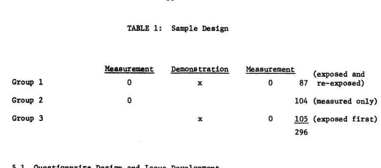
To test the reaction of farmers to the demonstration installations, re-lative to their reaction to a descriptionwe collected data from two groups of respondents. These respondents were randomly selected from farmers who were attending Farm Tractor and Safety Day at the University of Nebraska's

experimental farm at Mead. It was here that the PV irrigation demonstration was to take place and be viewed for the first time.

The two groups of respondents were:

1. Farmers who had not been exposed to the PV demonstration; 2. Farmers who had ust been through the demonstration.

A third set of measurements was taken from those who had been interviewed prior to viewing the demonstration and who returned to be reinterviewed after they had viewed the demonstration.

(36)

TABLE 1: Sample Design

Measurement Demonstration Measurement

(exposed and

Group 1 0 x 0 87 re-exposed)

Group 2 0 104 (measured only)

Group 3 x 0 105 (exposed first)

296

5.1 Questionnaire Design and Issue Development

An unstructured questionnaire was.developed, including the measurements we needed on sector demographics, price-acceptance distribution, number of

successes prior to adoption, cost delline factors and average sizes of

-installations.

-In addition, we used this opportunity to probe other areas and issues that would assist in future demonstration designs and marketing research in other sectors.

As part of this design, two project members went to Lincoln, Nebraska to interview a cross-section of individuals who were involved and knowledgeable about farm management and irrigation.

The people interviewed were:

1. A farm business writer, who also owned a small farm; 2. A large farm owner-operator;

3. A farm-extension county agent for the state; 4. A farm machinery dealer;

5. A bank farm loan officer;

(37)

7. The Department Head of Agricultural Engineering at the University of Nebraska;

8. University of Nebraska Professor of Agriculture and Water Resources;

9. University of Nebraska Public Relations and Communications editor in charge of the PV demonstration project;

10. Radio and T.V. station farm editors in Lincoln.

These interviews provided the basis to develop a set of questions addressing important irrigation issues.

A questionnaire draft was completed after these interviews. This draft was tested on farms in rural Massachusetts and New Hampshire. Modifications to the questionnaire and instructions to interviewers were made and the final questionnaire/interviewer instructions were finalized and printed.

5.2 Logistics

Field interviewers were contracted through a market research interviewing firm. This provided the project with 21 professional interviewers, from Lincoln or Omaha, Nebraska. Three members of the project staff acted as interviewer trainers and supervisors.

During the initial trip to Nebraska, arrangements for site location and facilities were made in cooperation with the Lincoln Labs of MIT and University of Nebraska. The best location would be one close to the demonstration site but on a route that would enable prospective respondents to the inercepted before arriving and after leaving the PV demonstration. The traffic pattern for the PV demonstration enabled this selection without problem (see

(38)

PARKI NG

ARI

Ecui PMEWT

DISPLAYS

(iN

au

I

P,

D'S PLAYS

ON F11104

EQU\PMENT

v

'

v

DI

SPLY

D. VN Y

Y

)(1"'tEL)

CORN FIELD

V

:Y

V

)f

Y

V+

INTERVIEWSITE

15 MILES

FRDM

MAINFUNCT

ION

AREA AND PV DEMO

SITE

Figure 6: PV, Mead, Nebraska Demonstration Site

The temperature was in the high 90's at the time and our air conditioned trailers aided in obtaining cooperation.

5.3 Execution and Supervision

The trailers were clearly identified with signs indicating their associa-tion with the PV project:

"M.I.T. - U. of N. INTERVIEW CENTER"

The interview required 20-30 minutes to complete depending upon the group being interviewed.

In order to insure understanding and proper execution of the interviewing, three project members circulated among the interviewers as they worked with respondents both inside and outside of the trailers.

-32-t.

0 F

tu

7 U. I11z

I

.

k

l ~ ~ ~ ~ ~ ~ ~ ~ _ II... ... I I l-- i J I _ I & U

nnrw

C rl r v

(39)

-Completed interviews were spot checked for completion. A running tab of interviews, by group, was maintained. Interviewers were directed from time to time to focus on specific groups in order to provide proper balance.

During the morning, announcements were made at the Main Function area promoting cooperation of the farmers with the interview center. Inter-viewers were identified with a tag and red "Interviewer" ribbons indicating their MIT.University of Nebraska PV association, their name and interviewer number.

A total of 296 interviews were completed between 8:30 a.m. and 4:00 p.m., as indicated in Table 1.

(40)

-34-6. Data Analysis

As indicated earlier, this document gives a quick read of the results of the Mead experience. This section reviews the data collected. The next two shows how the data can be used to calibrate the model for the agriculture

sector.

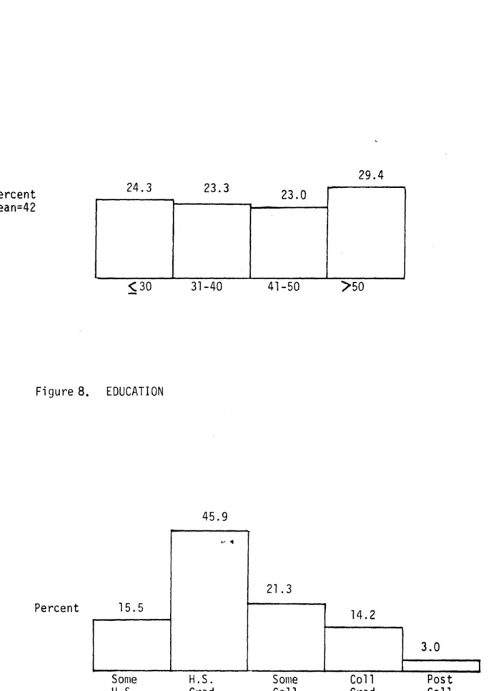
The farmers in the field study were a diverse group. Figure 7 shows a wide distribution of ages, with an average of 42 years old. Figure 8 indicates that nearly half have graduated only from high school, though 38.5% have some college experience. From Figure 9 we see that most of this education is farm related as 30.4% of the total, or 79% of those with college courses, have taken an agriculture course. These numbers are 25.5% and 66% respectively for business courses. For 76% of the farmers, according to Figure 10, farming is their only occupation, and from Figure ll, 72% have

spent more than 10 years on their farm, and average of 24 years on the farm. There is a wide range of sizes of farms according to Figure 12 with 52.2% of the farms 400 acres or less, but enough very large farms to pull the average up to 60%. Farming income is rather low, with 45% of the farms grossing under $40,000, according to Figure 13. Figure 14 shows 46.3% of the farms in this sample are irrigated, by a variety of methods, (Figure 15), using a variety of fuels (Figure 16), with more than half of those who irrigate using diesel fuel at least part of the time. Because the distribution of acreage is skewed, the distribution of irrigation fuel costs is also. Though 65.0% of the irrigators spend $3000 or less on fuel, the average expenditure is $4920, according to Figure 14.

(41)

Figure 7. Percent Mean=42 AGE IN YEARS

<30

Figure 8. EDUCATION 45.9 Percent 15.5 21.3 14.2 3.0

Some H.S. Some Coil Post

H.S. Grad Coil Grad Coll

24.3 23.3 23.0_{_3.(} 29.4

>50

31-40 41-50 l . . . L -. . . Nv.V

(42)

-36-Figure 9. COLLEGE COURSE

Percent 69.0 30.4 Yes Agriculture 74.5 No 25.5 Yes Business

Figure O. FARMING AS SECOND OCCUPATION?

Percent 76.0

24.0

No Yes

No

(43)

-Percent

Mean=24 28.0

z10

19.3

I

11-20

Figure 12. ACRES ON FARM

34.3 -.

-

la 201-400 401-800 23.3 21-30 31-40

>40

Percent Mean=607 - 17. 9 1

.5_

F

. r , ,, .l.

< 200

>

800

(44)

-38-Figure 13. GROSS FARM INCOME (K$)

Percent 17.7

<25

Figure 14. Percent 27.4 25-40 23.6 40-75 Irrigate? 53.7 No Yes 21.5 6.6 75-150 3.0 150-300

>

300

46.3 !~~~~~~~~~~~ , .- .

- ---

.i_ I I

(45)

Figure 1.. IF IRRIGATE, METHOD USED

(percefRt adds up to more than 100 du. to multiple responses)

Percent 64.8

Gated

46.3

Pivotal Other

Figure 11. IF IRRIGATE, FUEL USED

(percent adds up to more than 100 due to multiple responses)

Percent 51.2

14.8

42.6

1

35.8

Gas Propane Electric

32, 7 . 11 . S . . r Other Diesel

(46)

-40-Figure 17. FUEL COST ($) IF FARM IS IRRAGATED

Percent Mean=$4920 36.4 28.6 10.5 7.7 1 ,5 1500 1501-3000 3001-4500 4501-6000 6001-10,000 >10,000

Figure 18. MINIMUM SYSTEM DURABILITY IN YEARS NECESSARY FOR ADOPTION

42.4

Percent Mean=14.8 8.9 14.5 25.3 8.9

---

-~~I

<10~

~~~~~~

_101.51

~~~~~~

02 ~~~~~~~~~~~~~~~~~~~~~~~~~~

2

9.1 7.7 , @ . _ _~~~~~

~

--- I ._ .-I 1 I II

<10

10-14 15-1 9 20-24 2 5

(47)

Figure 19. MAXIMUM PAYBACK PERIOD IN YEARS NECESSARY FOR ADOPTION 42.0 Percent Mean=8.8 11.5 __, 5-9 33.5 10-14 6.7 15-19 6.3 20

Figure 20. MINIMUM NUMBER OF PRIOR SUCCESSFUL INSTALLATIONS NECESSARY FOR ADOPTION Percent Mean= 4.5 34.5 1-2 3-5

!

,.~~~~~~~

l i .~~~~~~~~~~~~~~

I

I I 6-10 2> I 0

(48)

What do the farmers as a group expect from an irrigation system? These are key questions needed to calibrate equations such as (13) in our accept-ability model. 56.9% of the farmers expect it to last at least 10-19 years under normal use (Figure 18), with an average of 14.8 years. More than half of them, 53.5%, expect a system to pay itself back in less than 10 years, 8.8 years on average (Figure 19). Most of the farmers need to see only a few successful installations before they would be willing to buy a system themselves (Figure 17). 34.5% are willing to be first in their area to buy a system, and 53.3% would be convinced by 2 or fewer successful installations. However, there are enough skeptics to push the average up to 4.5 installations.

Perceptions of irrigation systems (displayed in Figure 21-23) offer few surprises. Photovoltaic systems score very well in reducing pollution, saving resources and protection against fuel rationing, and very poorly on cost, weather sensitivity and technical maturity. By contrast, the conventional systems score well on being simple, mature technologies. The perceptual differences between farmers exposed to the demonstration project and those

who were not are not great. Though feelings that photovoltaics saves resources, reduces pollution, etc., were enhanced, there was no change in the degree to which the farmers were willing to consider such a system. Similarly, though perceptions of the conventional systems' societal value fell after seeing the demonstration, the degree of consideration didn't significantly change. It is interesting to note that the responses to questions 6, 7, and 14, all about energy savings, pollution and rationing had much less variation for PV than for combustion or electric, or indeed, other PV questions.

(49)

Figure 21la Perceptions of Photovoltaics System

Agree 1. The system provides reliable power

for irrigation.

2. Adoption of the system protects against power failures.

3. Performance of the system is

sensi-tive to weather conditions.

4. The system is flexible enough for multiple uses on the farm.

5. The system is more expensive to maintain than other systems.

6. The system protects against farm fuel rationing.

7. The system allows us to do our part in reducing pollution.

8. The system uses too many concepts that have not been fully tested.

1I

_

Disagree -_ I . I I I I I

II

I1

/ / ., / / I .~' I 1 1, l . I I

\

I I 1 ~ J; I I Il / I it 1 I . I I ' I

PreExposu-

re=

Post Exposure

---~~~~~~~~~~~~~~~~~~~

I I I I

(50)

-44-Figure 21b. I'erceptions; of Photovoltaics System (Continued)

Agree

9. Installation of the system is

too costly.

10. The system is too complex.

11. The system is visually

unattractive.

12. The system is subject to weather damage.

13. Other forms of energy will be

available in the future which make the system unnecessary.

14. The system leads to considerable savings of energy resources.

15. If the experts approved and

recommended a system, I would seriously consider it.

16. The system requires changes in conventional farm practices.

I 1 I I I I '\ I I -y1 .1 1 \ \ Is I .. ...

k

L lI

1

I I I I I / // // I .l I l ,I l

\\~

Pre por--- = Post Exposure Disagree

(51)

Figure22a. Perceptions of Combustion System

for irrigation.

3. Performance of the system is

sensi-tive to weather conditions.

4. The system is flexible enough for

multiple uses on the farm.

8. The system uses too many concepts that have not been fully tested.

I .- l I I I I I I 1 1 . ai I I I .. I I.. _I I I . I I - -1 1ia I I I

i

-

i

-

7 9

I

1 -

--I I - I __ - I- I 'J1 I . .II N . %

Pre E posure- …= Post Exposure Disagree

(52)

-46-Figure 22b. Perceptiolls of Combustion System (Continued)

Agree

too costly.

11. The system is visually unattractive.

12. The system is subject to

weather damage.

PreEpose--- = Post Exposure

Disagree I I I L , J I J I I I I I 1. I I ! I I 11 I ,1 .I I I I I I I I I I I I I I 1l ... I l l

I

-

A -

I

L\

= Pre Exposure

(53)

Figure 23a. Perceptions of Electric System

for irrigation.

3. Performance of the system is sensi-tive to weather conditions.

4. The system is flexible enough for multiple uses on the farm.

8. Tilhe system uses too many concepts that have not been fully tested.

I*-

/ I / I 1

<

I

~ J

J

I)

1 1

~~~~~I

\~~~~~~~~~~~

I

IJ

*

~//

I_ I I I J 1 = Post Exposure Disagree I _ I

---I I I I

=Pre Exposure

(54)

-48-Figure .23b. Perceptions of Electric System (Continued)

Agree

too costly.

11. The system is visually unattractive.

12. The system is subject to

weather damage.

\ / /

I .I

I

1 /

.

/x // I I .1 1l) / / I 1 1/ / 1 1I I I I I ... k

= Pre Exposure

---

= Post Exposure

(55)

Figure 24. PV CHOICE Percent

Before

I-

After 3m 45.3

32.1

Al 0 Second

31.7

26.5 22.6

First

Third

(56)

-50-Figure 25. PERCENT INCREASE WILLING TO PAY FOR PV

Percent

Before |

Median=50 for both

21. After 36.2 30.3 11.8 11.0 25 25-49 50-74 75-99 100

Figure 26. ACTION IN ENERGY SHORTAGE IF PV AVAILABLE

Percent Before I After R 43.5 B uy 20.1 18.1 Follow Others 17.3 18.6 Other 20.5 22.1 26.8 19.2

H

Wait I I I I 1

(57)

When it came to choosing among the three systems, exposure to the demonstration seems to have made little difference. The farmers generally chose photovoltaics about the same after exposure, (Figure 24). The percent increase in initial cost the farmers are willing to pay also seems unaffected by exposure (Figure 25). For both pre- and post-exposure the median increase is 50 %.

Finally, Figure 26 shows that, following exposure, nearly half the sample would buy photovoltaics in an energy shortage.

These data show that:

- PV is understandable;

- PV is acceptable to a wide variety of farmers; - A premium would be paid for the product;

(58)

-52-7. PV Preference and Perceptual Analysis

Factor analysis is used to determine the key perceptual dimensions farmers use to assess irrigation systems. Consumers may be able to respond to an unlimited number of questions about a topic; yet, in their minds, they may structure information into only a few, key underlying dimensions. We refer to these dimensions as evaluation criteria. We must test to see if these evaluation criteria were equal for the three groups that were sampled: those responding only to the post-test survey, those responding only to the pre-test survey, and the group responding to the pre-test and post-test surveys.

The first step is to factor analyze the results for all respondents within the respective subgroups. From the results of the factor analysis, we can determine whether the dimensionalities of the evaluation spaces are

the same for each of the subgroups. If the dimensionalities are indeed equal, we can determine whether the evaluation criteria are similar across subgroups by employing the test discussed in Choffray and Lilien [10]. The test measures whether the factor score coefficients used to measure the

scores for each individual on a given factor are the same for the two groups. Item responses for each of the three subgroups were factor analyzed. Factors were extracted using the criterion that eigenvalues must be greater

than or equal to 1.0. In addition, certain combinations of these subgroups were factor analyzed to be consistent with the requirements for the test. For the following discussion we denote:

pre-test and post-test survey = Group A pre-test survey only = Group B post-test survey only = Group C

(59)

Our analysis suggested that all groups seemed to have perceptual spaces of dimensionality 3, the number of factors extracted for each group.

First we test Group A vs Group C. This comparison reveals if there is a significant effect from exposure to the pre-test questionnaires. The

results of this comparison (summarized in Appendix 1) indicate that the evaluation criteria exhibited by Groups A and C are essentially similar.

Analysis of the similarity between Groups B and C was undertaken to assess the effect of respondents inspecting a PV site on their evaluation

criteria. The results of comparing factors that load on similar variables between B and C (summarized in Appendix 1) reveal significant dissimilarities. Therefore, we can state that the evaluation criteria of the group that was only exposed to a concept statement are different from the evaluation criteria of the group that was exposed to the PV site.

For simplicity we can roughly name the factors for all these groups as:

1. Newness/Expense

2. Complexity/Untried Concepts

3. Independence from Traditional Fuel Sources

The preference regressions, discussed below, suggest that factor 2 is the factor of key importance in explaining preference.

We are now concerned with how perceptions are related to preferences; thus, we use preference regression analysis to determine how these evalua-tion criteria are related to system preferences.

Individuals were asked to rank their system preferences assuming that each of the alternatives satisfied the respondent's minimum requirements for

system payback period, system life and the number of prior locations. These rank preferences were regressed against the corresponding factor scores

(60)

-54-using ordinary least squares, for the sample groups B and (A+C). The regres-sion equations for both groups are shown in Appendix 2. The preference

paramters for both equations are significantly different from zero at the 90% confidence level and all appear to have the correct sign except for the preference parameter for factor 1 for group (A+C). Analysis of the relative importance of the questionnaire items for group (A+C) revealed that the

nega-tive sign of the preference parameter for factor 1 is explained by the fact that the importance of protection against fuel rationing outweighs the nega-tive characteristics of high initial cost, system complexity and system new-ness which are also found in factor 1.

Using the regression equation we predicted the system preferences for each of the respondents (predictions were only made for individuals who had ranked all three systems). The percentage of correct predictions for first preference recovery are shown in Figure 27. The results indicate that the model is useful in predicting individual preferences.

To determine the relative importance of each of the items to the re-spondents in groups B and (A+C), the preference parameters were multiplied by the corresponding factor score and summed up across each item. This

tells what the effect of a unit change in one of the original items is pre-dicted to do to preference. (If an item were only to load on one factor, at a unit level, this would be equivalent to examining the size of the regres-sion coefficient.) The results of these calculations are shown in Figures 28

and 29.

The results indicate that by exposing potential users to an opera-tional PV powered irrigation system we are able to lower their concerns that a PV system contains "too many untried concepts" and is "visually

(61)

unattractive." Also, after exposure to an operating PV system, protection against fuel rationing and system reliability become the two most important criteria. Since a PV system provides greater protection against fuel ration-ing than either of the other two systems under consideration, one would

assume that a higher percentage of individuals in group (A+C) would prefer the PV system than the individuals in group B. This hypothesis, however, is not supported by the data from the questionnaire. 32.1% of the respon-dents in group (A+C) ranked the PV system first in comparison to 31.7% for group B. The percentage of respondents ranking PV second was 45.3% for group (A+C) and 41.8% for group B.

From the above data we can conclude that exposure to an irrigation system powered by a PV energy source will change a potential user's

evalua-tion criteria. However, it will not have an impact on their system prefer-ences even when it is assumed that the PV system satisfied their minimum

system requirements.

Additional preference analyses were performed including age, farm size and education of the farmer. These variables did not add to the predictive or explanatory power of the model, suggesting that the perceptual (factor analysis) data does a good job in explaining individual preferences.

(62)

-56-Figure 27

Model Predicted Preference Recovery

GROUP B (Not Exposed to Site)

1st Preference Full Preference

Recovery

.Recovery

.597 .388

(expected = 0.337) (expected = 0.167)

l GROUP (A + C) (Exposed to Site)

1st Preference Full Preference

Recovery

.528 .352

(63)

Figure 28

Rank of Variables in Order of Importance to Respondents

GROUP B

(Not Exposed to Site)

RANK DESCRIPTION

1 'leads to considerable savings of energy

2 system is too complex

3 system contains too many untested concepts

4 system is visually unattractive

5 system protects against power failures

6 expert approval & recommendations prior to consid.

7 system reduces pollution

8 provides reliable power for irrigation

9 protects against fuel rationning

10 system installation too costly

11 system flexible for multiple use

12 sys. requires change in conventional farm practices 13 future forms of energy will make system unnecessary 14 system more expensive than others to maintain

15 system is subject to weather damage

(64)

-58-Figure 29

Rank of Variables in Order of Importance to Respondents GROUP (A + C)

(Exposed to Site)

RANK DESCRIPTION

1 protects against fuel rationing

2 provides reliable power for irrigation

3 system is too complex

4 expert approval & recommendations prior to consideration

5 system reduces pollution

6 leads to considerable savings of energy