HAL Id: insu-01399827
https://hal-insu.archives-ouvertes.fr/insu-01399827
Submitted on 21 Nov 2016
HAL is a multi-disciplinary open access
archive for the deposit and dissemination of sci-entific research documents, whether they are pub-lished or not. The documents may come from
L’archive ouverte pluridisciplinaire HAL, est destinée au dépôt et à la diffusion de documents scientifiques de niveau recherche, publiés ou non, émanant des établissements d’enseignement et de
Laboratory micro-seismic signature of shear faulting and
fault slip in shale
J Sarout, Yves Le Gonidec, D Ougier-Simonin, D Schubnel, Y. Guéguen, D.N.
Dewhurst
To cite this version:
J Sarout, Yves Le Gonidec, D Ougier-Simonin, D Schubnel, Y. Guéguen, et al.. Laboratory micro-seismic signature of shear faulting and fault slip in shale. Physics of the Earth and Planetary Interiors, Elsevier, 2017, 264, pp.47-62. �10.1016/j.pepi.2016.11.005�. �insu-01399827�
Accepted Manuscript
Laboratory micro-seismic signature of shear faulting and fault slip in shale J. Sarout, Y. Le Gonidec, A. Ougier-Simonin, A. Schubnel, Y. Guéguen, D.N. Dewhurst
PII: S0031-9201(16)30270-9
DOI: http://dx.doi.org/10.1016/j.pepi.2016.11.005
Reference: PEPI 5984
To appear in: Physics of the Earth and Planetary Interiors
Accepted Date: 16 November 2016
Please cite this article as: Sarout, J., Gonidec, Y.L., Ougier-Simonin, A., Schubnel, A., Guéguen, Y., Dewhurst, D.N., Laboratory micro-seismic signature of shear faulting and fault slip in shale, Physics of the Earth and Planetary
Interiors (2016), doi: http://dx.doi.org/10.1016/j.pepi.2016.11.005
This is a PDF file of an unedited manuscript that has been accepted for publication. As a service to our customers we are providing this early version of the manuscript. The manuscript will undergo copyediting, typesetting, and review of the resulting proof before it is published in its final form. Please note that during the production process errors may be discovered which could affect the content, and all legal disclaimers that apply to the journal pertain.
Laboratory micro-seismic signature of shear faulting
and fault slip in shale
J. Sarouta , Y. Le Gonidecb , A. Ougier-Simoninc , A. Schubneld , Y. Gu´eguend , and D.N. Dewhursta a
CSIRO Energy, Perth, Australia
b
G´eosciences Rennes - CNRS/INSU UMR6118, Rennes, France
c
British Geological Survey, Engineering Geology, Keyworth, UK
d
Ecole Normale Sup´erieure, CNRS-UMR 8538, Laboratoire de G´eologie, Paris, France
Abstract
This article reports the results of a triaxial deformation experiment con-ducted on a transversely isotropic shale specimen. This specimen was instru-mented with ultrasonic transducers to monitor the evolution of the micro-seismic activity induced by shear faulting (triaxial failure) and subsequent fault slip at two different rates. The strain data demonstrate the anisotropy of the mechanical (quasi-static) compliance of the shale; the P-wave velocity data demonstrate the anisotropy of the elastic (dynamic) compliance of the shale. The spatio-temporal evolution of the micro-seismic activity suggests the development of two distinct but overlapping shear faults, a feature similar to relay ramps observed in large-scale structural geology. The shear fault-ing of the shale specimen appears quasi-aseismic, at least in the 0.5 MHz range of sensitivity of the ultrasonic transducers used in the experiment. Concomitantly, the rate of micro-seismic activity is strongly correlated with the imposed slip rate and the evolution of the axial stress. The moment
tensor inversion of the focal mechanism of the high quality micro-seismic events recorded suggests a transition from a non-shear dominated to shear-dominated micro-seismic activity when the rock evolves from initial failure to larger and faster slip along the fault. The frictional behaviour of the shear faults highlights the possible interactions between small asperities and slow slip of a velocity-strengthening fault, which could be considered as a realistic experimental analogue of natural observations of non-volcanic tremors and (very) low-frequency earthquakes triggered by slow slip events.
Keywords: Shale, P-wave velocity, Anisotropy, Micro-seismicity, Focal mechanism, Shear faulting, Fault slip, Friction
1. Introduction
1
Changes in the stress state can induce brittle damage and fracturing in
2
rocks that can radiate mechanical energy in the form of elastic waves. At the
3
field scale, the radiated energy is often referred to as Micro-Seismic (MS)
ac-4
tivity; in the laboratory, it is often called acoustic emissions [28, 31, 32]. The
5
phenomena of micro-seismicity and acoustic emission are similar in nature,
6
although the frequency content of the radiated elastic perturbation might be
7
different due to the scale of the fracturing. Therefore, in this manuscript we
8
will use the term micro-seismicity (and its derivatives such as micro-seismic
9
activity or micro-seismic events) to name the events recorded in the
labo-10
ratory. In general, the accumulation of damage can ultimately lead to the
11
mechanical failure of the rock. Among the various rock failure mechanisms
12
listed in the literature, we focus here on brittle faulting pertaining to
nu-13
merous geological settings observable during the deformation of rocks in the
14
Earth’s upper crust.
15
It is generally accepted that for a given material, MS activity is
promi-16
nently observed during deformation under the following conditions: (i)
rel-17
atively low normal stresses; (ii) relatively high shear stresses; and/or (iii)
18
relatively high stress loading rates, e.g., [1, 51]. In the past, most research
19
efforts published in the literature involving micro-seismic monitoring of
de-20
formation processes in the laboratory have focused either on:
21
- crystalline rocks in relation to earthquake/fault mechanics, geotechnical or
22
geothermal applications, e.g., [6, 26, 29, 33]; or
23
- conventional reservoir rocks in relation to oil and gas exploration,
pro-24
duction and monitoring (reservoir integrity, compartmentalisation,
induced fracture/fault reactivation...), e.g., in sandstones [7, 8, 9, 15, 17, 45];
26
or to a lesser extent in porous carbonate rocks [16].
27
At the field scale, several studies on the monitoring of MS activity in
28
granites and carbonates have been published. These include the monitoring
29
of: thermally-induced MS activity potentially associated with radioactive
30
waste disposal in boreholes drilled in a tunnel’s floor at ¨Asp¨o’s Hard Rock
31
Laboratory in Sweden [37], in the Excavation Damage Zone (EDZ) in the
Un-32
derground Research Laboratory in a granitic rock mass in Canada [53, 54]
33
and injection-induced MS activity in a limestone formation in the Laboratoire
34
Souterrain `a Bas Bruit in France [18]. Fewer field-scale studies on the MS
35
activity induced by faulting or fault slip in shale formations have been
pub-36
lished. A recent study demonstrated the feasibility of monitoring the time
37
evolution of MS activity associated with the EDZ in the Opalinus Clay
for-38
mation at the Mont-Terri Underground Research Laboratory in Switzerland
39
[27]. The MS activity associated with fluid injection in the Colorado Shale
40
formation was successfully monitored by [46]. In contrast, the monitoring of
41
the spatial extent of anthropogenic hydraulic fractures in stimulated oil/gas
42
reservoirs have been an active field of research since the 1980’s, strongly
sup-43
ported by industry funding, especially in the recent years with the advent
44
and development of commercially-viable unconventional reservoirs such as
45
gas shales, e.g., [49].
46
At the laboratory scale, experiments have been reported on shales
uni-47
axially deformed at room conditions under large loading rates (see [2] and
48
references therein). However, no determination of spatial locations or focal
49
mechanisms of the recorded MS events (MSEs) was carried out. MS activity
and location in shale samples containing quartz veins have been reported by
51
[30]. In this particular case, and as expected, the MS activity seemed to
52
coincide with the location of quartz veins favorably oriented with respect to
53
the maximum principal compressive stress.
54
To our knowledge, no data on spatio-temporal localisation and focal
55
mechanism estimation of MS activity have been reported on deforming
clay-56
rich rocks such as conventional reservoir-sealing shales. Under triaxial
defor-57
mation at realistic subsurface stress conditions, the shale specimens fail in
58
shear, leading to the formation of a shear fracture. The first questions that
59
arise then for these rocks are the following: (i) can we expect precursory
60
micro-seismic activity prior to the macroscopic faulting? (ii) Would the slip
61
on the newly generated fault induce any micro-seismic activity? (iii) How
62
would the signature of the MS activity be affected by the deformation rate?
63
Due to their fine-grained nature, it is generally thought that clays act as a
64
lubricant in frictional geological environments, e.g., [36]. Also, the brittleness
65
of clay behaviour is known to be controlled by their degree of hydration (the
66
more hydrated, the less brittle), their mineral composition, and the imposed
67
deformation rate (higher rates induce a more brittle response). The lack
68
of published experimental studies on the MS activity of shales subjected to
69
stress conditions typical of the upper crust can probably be explained by the
70
inherent complexity of shales and the associated difficulty in conducting
lab-71
oratory deformation experiments on them under well-controlled conditions.
72
In addition, there is considerable technical complexity in conducting and
pro-73
cessing laboratory experiments aimed at monitoring and locating with high
74
accuracy the MS activity induced by deforming relatively small specimens.
In this regard, the difficulty in locating the MS activity is exacerbated by
76
the directional dependency (anisotropy) of wave propagation in shales, e.g.,
77
[11, 13, 24, 39, 40, 48].
78
In this paper, the results and analysis of a laboratory deformation
experi-79
ment in a shale specimen are reported. The specimen was triaxially deformed
80
to beyond the failure point under subsurface stress conditions while
associ-81
ated MS activity was recorded. The aim was to analyse the contrast in the
82
MS signature of shear faulting and subsequent fault slip as well as the effect
83
of the deformation rate on the fault’s micro-seismic and frictional response.
84
In the following pages, the experimental conditions are detailed (section
85
2) along with the main results in terms of stress-strain data, ultrasonic
P-86
wave velocity data, and micro-seismic activity (section 3). The fourth section
87
is dedicated to an analysis and discussion of these results in terms of the MS
88
signatures of shear faulting and fault slip (slow/fast slip), frictional behaviour
89
of the shear fault in relation to the associated MS activity, and a comparison
90
to other rock lithologies.
91
2. Description of the experiment
92
2.1. Shale material
93
A large core was recovered from the North Sea at a depth of 1643 m
be-94
low sea bed in a clay-rich shale formation (Campanian, upper Cretaceous).
95
The core was preserved since recovery from depth in several layers of plastic
96
and aluminium wrap with an additional external wax coating. After
unpack-97
ing, this shale appeared relatively homogeneous, dark grey in colour, with
98
bedding visible inclined at 45◦ to the core axis. Twin cylindrical specimens 99
40 mm in diameter have been cored along the axis of the original core so
100
that the bedding was also inclined at 45◦ to their axis. Their end faces were 101
trimmed and ground to be parallel to each other to within 0.02 mm. The
102
final length of the specimens was 81 mm (long specimen) and 40 mm (short
103
specimen), respectively. For the coring, trimming and grinding operations,
104
compressed air was used as the cooling fluid. After preparation, the
spec-105
imens were equilibrated for several days at room conditions (20◦C, relative 106
humidity of 50%) until stabilisation of their mass at these conditions. After
107
this initial treatment the specimens turned to a light grey colour. The mass
108
evolution of the samples during this initial treatment and their change in
109
color suggest that they lost water (dehydration) by exchange with the
atmo-110
sphere. The porosity of the shale was estimated to be of the order of 19%
111
(density: 2370 kg/m3
) based on mass measurements conducted on a separate
112
block cut from the original core in its preserved state (immidiately after
un-113
packing the core) and its state after mass stabilisation at a room conditions
114
(20◦C, relative humidity of 50%). Note that this porosity is only a lower 115
bound estimate of the actual porosity of the shale assuming that the core
116
was fully water-saturated in its preserved state and is fully dry in its final
117
equilibrated state (20◦C and relative humidity of 50%). It is expected that 118
only the so-called ”free” water could have evaporated during this treatment,
119
so that the shale specimens are likely in a partially saturated state.
120
The shorter specimen was used to conduct permeability measurements
121
with nitrogen gas under increasing effective pressure using a steady state
122
method, i.e., constant gas flow imposed at one end of the specimen, and
123
monitoring of the differential pressure build-up and stabilisation across its
two ends [25]. The permeability results are summarised in TABLE 1. The
125
permeability of this shale to nitrogen decreases by almost two orders of
mag-126
nitude from 2.1×10⁻⁵mD down to 6.9×10⁻⁷ mD when the effective confining 127
pressure increases from 4 MPa up to 65 MPa. This seems to indicate that
128
stress-sensitive pre-existing micro-cracks (damage) are closed by the
increas-129
ing effective pressure. Such micro-cracks might have been induced by stress
130
release following the recovery of the shale core from depth and/or the
dehy-131
dration of the specimen at room conditions during initial treatment.
132
The longer specimen was used to conduct the triaxial deformation
exper-133
iment with MS monitoring detailed in the remainder of this article.
134
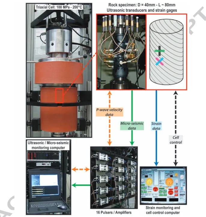
2.2. Experimental equipment
135
In order to characterise the MS response of the shale to changes in the
tri-136
axial stress state, a specific laboratory setup is required to monitor both the
137
deformation of the specimen and the induced MS activity. The experimental
138
setup consists mainly of: (i) a Sanchez Technologies axisymmetric triaxial
139
stress vessel in which a radial and an axial stress can be independently applied
140
to a cylindrical rock specimen; (ii) an Applied Seismology Consultants
multi-141
channel ultrasonic/micro-seismic monitoring system (Fig. 1). This apparatus
142
allows the simultaneous acquisition of various types of data on a single rock
143
specimen: (i) radial and (ii) axial deformations, (iii) active ultrasonic
moni-144
toring, i.e., ultrasonic P-wave velocities along numerous propagation paths at
145
selected stages of the deformation (called velocity surveys); and (iv) passive
146
monitoring, i.e., induced micro-seismicity (also called acoustic emissions).
147
Note that both active and passive monitoring are conducted using the same
148
array of ultrasonic transducers as described below.
After the initial drying treatment of the long shale specimen at a
temper-150
ature of 20◦C and a relative humidity of 50%, four strain gauges are glued 151
onto its lateral surface so that four independent directions of deformation
152
are measured (see Figs. 1 and 2): Gauge 1 measures the axial strain along
153
the specimen’s axis, at 45◦ to the bedding orientation. Gauge 2 measures 154
the circumferential strain orthogonal to the specimen’s axis, at 45◦ to the 155
bedding; this strain also corresponds to the radial strain, and for sake of
156
simplicity, it will be referred to as radial strain in the remaining of the
ar-157
ticle. Gauge 3 measures the strain orthogonal to the bedding, at 45◦ to the 158
specimen’s axis. Gauge 4 measures the strain along the bedding, at 45◦ to 159
the specimen’s axis. In addition, the average axial displacement between the
160
two ends of the specimen was monitored using three contactless Eddy current
161
displacement transducers located outside the pressure vessel.
162
2.3. Experimental protocol
163
The shale specimen is inserted into a flexible Viton sleeve and placed
164
inside the pressure chamber of the triaxial stress vessel, which is then closed
165
and filled with oil. The purpose of the flexible sleeve is to isolate the specimen
166
from the hydraulic oil used to apply the radial stress [40]. This specimen is
167
instrumented with: (i) four strain gauges glued directly to its lateral surface,
168
at mid-height; (ii) an array of 16 miniature ultrasonic transducers (6 mm in
169
diameter) made of piezo-ceramic material with a central resonant frequency
170
of about 0.5 MHz. These transducers can be used as ultrasonic sources or
171
receivers attached directly to the lateral surface of the specimen, through
172
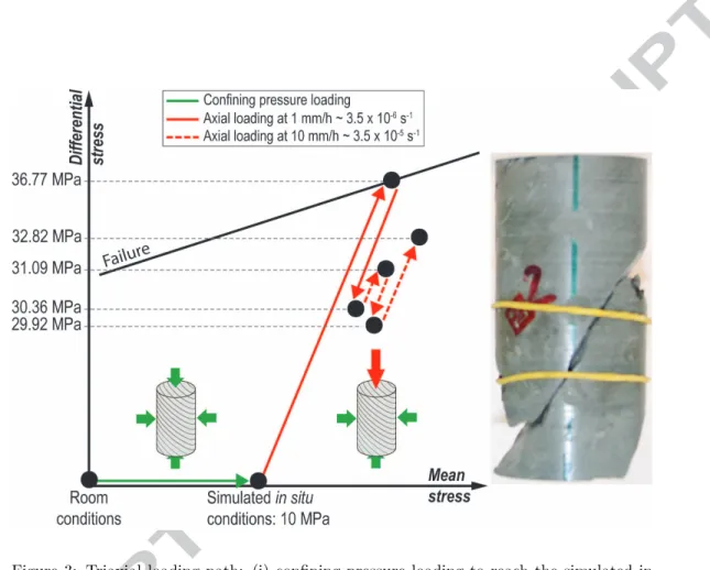
sealable holes in the flexible Viton sleeve (Fig. 2).
173
The experimental deformation protocol consists of: (i) an isotropic stress
loading to subject the specimen to a simulated in situ condition with a
175
confining pressure of 10 MPa; (ii) a deviatoric stress loading at a constant
176
axial displacement rate of 1 mm/h (3.5×10⁻⁶ s−1) up to a point beyond the 177
specimen’s failure, which is indicated by a peak in the recorded deviatoric
178
stress; then (iii) a sudden increase of the displacement date to 10 mm/h
179
(3.5×10⁻⁵ s−1) until stabilisation of the recorded deviatoric stress (Fig. 3). 180
The deformation experiment is conducted without injecting water and
with-181
out controlling the pore pressure at the two ends of the specimen.
182
The aim of the deviatoric stress loading is two-fold: (i) assess the effect
183
of shear faulting and fault slip on the MS response of a shale; and (ii)
as-184
sess the effect of fault slip rate on the MS activity. The active and passive
185
monitoring equipment is controlled with the Xtream software, while the data
186
management and processing is conducted with the Insite Seismic Processor
187
software.
188
As part of the active ultrasonic monitoring, at selected stages of the
189
experiment, a P-wave velocity survey is conducted. Each survey consists
190
of 16 consecutive shots, one from each transducer acting as a source. For
191
each source transducer shot, the transmitted waveforms are recorded on the
192
15 remaining transducers which act as receivers. The waveform recorded at
193
each receiver corresponds to the mechanical vibration transmitted through
194
the rock specimen from the source transducer to that particular receiver. In
195
order to improve the signal-to-noise ratio (SNR), each waveform is in fact the
196
result of the stack of several tens of shots from a given source transducer. The
197
waveforms are recorded with a sampling rate of 10 MHz and an amplitude
198
resolution of 12 bits. Each source-receiver pair defines a particular ray path
within the specimen, i.e. different directions of wave propagation relative to
200
the specimen’s axis and therefore relative to the shale bedding. Each velocity
201
survey typically lasts 30 seconds and consists of 240 waveforms (recorded over
202
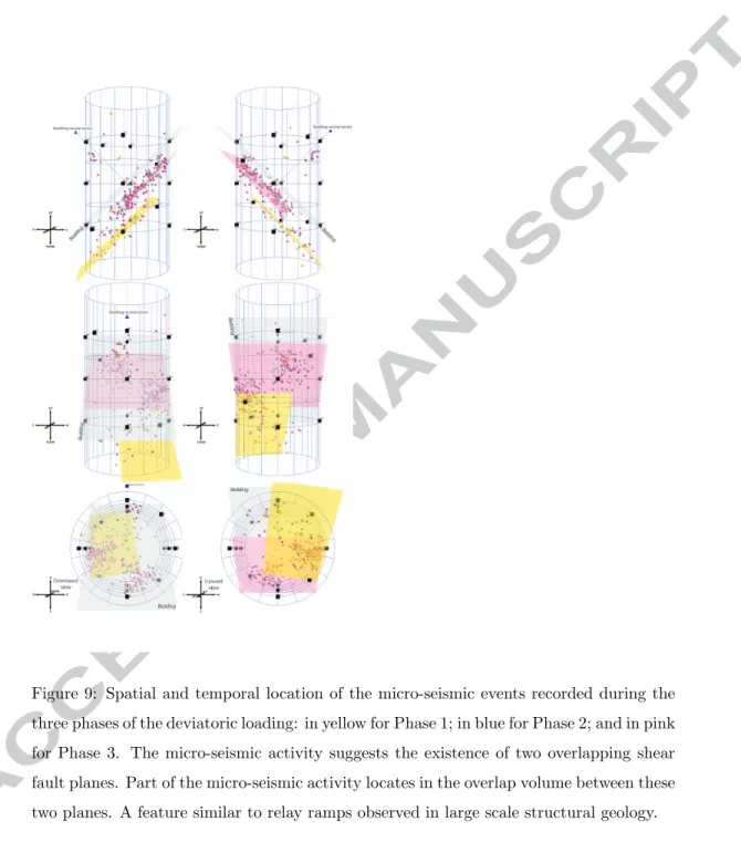
82 microseconds), half of which corresponds to different ray paths within the
203
volume of the specimen. The ultrasonic survey data set acquired during the
204
experiment consists of 10 surveys recorded during the isotropic stress loading
205
after every one or two MPa of confining pressure, and 11 surveys recorded
206
during the deviatoric stress loading.
207
Between two consecutive velocity surveys, the ultrasonic/micro-seismic
208
system is switched to the passive monitoring mode in order to record any
209
MS activity induced by the stress loading. In this mode, the voltages
gen-210
erated by the ultrasonic transducers sensing a given Micro-seismic events
211
(MSE) are recorded according to a pre-defined trigger logic. Typically, if five
212
transducers exceed a voltage threshold of 15 mV within a time window of
213
100 microseconds, the waveforms from all 16 transducers are recorded for a
214
time window of 82 microseconds. These waveforms are also recorded with a
215
sampling rate of 10 MHz and an amplitude resolution of 12 bits. At the end
216
of the experiment, nearly 500 events have been detected according to this
217
protocol.
218
3. Shear faulting and post-failure slip
219
3.1. Identification of the faulting dynamics
220
The shale deformation experiment can be divided into an isotropic stress
221
loading (Phase 0), followed by a deviatoric stress loading. The deviatoric
222
loading stage itself is composed of three phases as discussed below (Figs. 4
and 5).
224
During Phase 0, the specimen reaches the simulated in situ stress
con-225
dition with a confining pressure of 10 MPa (point A in Figs. 4 and 5).
226
This phase consists of a step-wise increase of the confining pressure and an
227
equilibration of the specimen at the target condition over several days.
228
Phase 1 corresponds to the shear faulting (yellow area in Figs. 4 and 5).
229
Axial loading is applied to the specimen at a controlled vertical displacement
230
rate of 1 mm/h until the peak axial stress is slightly passed and a first
231
moderate stress drop of about 1 MPa is observed, most probably concomitant
232
with a first slip of the newly formed shear fault (point B in Figs. 4 and 5).
233
The dip angle of the slip surface with respect to a horizontal plane have been
234
estimated post mortem to be about 45◦, coinciding approximately with the 235
orientation of the shale bedding. Such an orientation is probably due to the
236
presence of weak bedding planes (see failed sample in Fig. 3).
237
Phase 2 corresponds to the slow fault slip (blue area in Figs. 4 and 5). The
238
vertical displacement rate is maintained constant so that the newly formed
239
shear fault is slipping at constant rate, while the axial stress drop of about
240
7 MPa is more pronounced than in Phase 1.
241
Phase 3 corresponds to the fast fault slip (pink area in Figs. 4 and 5) The
242
vertical displacement rate is suddenly increased to 10 mm/h, which leads to
243
a sudden, moderate and temporary increase of the axial stress of less than 1
244
MPa (point C in Figs. 4 and 5). While the axial displacement is maintained
245
constant at that higher rate, after a temporary stabilisation, the axial stress
246
starts to slowly increase to reach a plateau by the end of the experiment
247
(point D in Figs. 4 and 5).
In addition to the evolution with time of the axial stress and displacement,
249
Figs. 4 and 5 also display the evolution of the micro-seismic activity in terms
250
of cumulated number of MSEs and rate of occurrence, respectively. Overall,
251
the cumulated number of events is linearly related to the axial displacement
252
rate, except temporarily after the increase in the imposed displacement rate
253
from 1 to 10 mm/hour and until the axial stress reaches a plateau.
Con-254
sistently, the rate of micro-seismic activity is strongly correlated with the
255
imposed displacement rate and the evolution of the axial stress. More
de-256
tails about this part of the dataset are provided in Section 4.3.
257
3.2. Analysis of the stress-strain data
258
At the end of the isotropic stress loading (Phase 0 aimed at reaching a
259
confining pressure of 10 MPa), Gages 1, 2, and 3 display a similar amount
260
of strain (0.123%), whereas Gage 4 (along the bedding and at 45◦ to the 261
specimen’s axis) displays about half that amount of strain (0.072%). This
262
suggests a significant stress-induced anisotropy of the shale in which the
bed-263
ding direction is significantly less compliant than the three other measured
264
directions. However, the difference in the magnitude of the recorded strain
265
between Gages 1, 2 and 3 does not clearly reflect a larger compliance in a
266
direction orthogonal to the bedding compared to the two other intermediate
267
orientations (at 45◦ to the bedding). Over all, the amount of deformation 268
experienced by the specimen during this isotropic stress loading is relatively
269
small, which may explain the lack of sensitivity of the strain gauge recordings
270
and therefore the lack of discrimination between the three directions probed
271
by Gages 1, 2 and 3.
272
During the deviatoric stress loading, the four gauges record a significantly
larger amount of strain (Fig. 6). The whole dataset recorded during Phases
274
1, 2 and 3 is displayed in this figure. Note however that past the point
275
of strain localisation (shear faulting, slightly beyond the peak stress
corre-276
sponding to Point B in Fig. 4-6), the local strain measurement provided by
277
the strain gauges is no longer representative of the average strain field over
278
the volume of the specimen because most of the imposed axial displacement
279
is then accommodated by the slipping shear fault. The largest deformation is
280
expectedly recorded along the specimen’s axis (about 1% at the peak stress,
281
along the maximum principal compressive stress), while the radial strain
282
along the minimum principal stress is negative due to Poisson’s effect (about
283
-0.1% at the peak stress). Gages 3 and 4 record an intermediate amount of
284
strain, consistent with their orientation with respect to the principal stress
285
axes. The difference in magnitude of strain recorded by these two gauges
286
highlights again the existence of a significant anisotropy in the mechanical
287
compliance of the shale. Indeed, in view of their similar orientation with
288
respect to the principal compressive stress axis (45◦), they should record a 289
similar deformation if the shale was isotropic. However, it turns out that
290
Gage 3 oriented normal to the bedding records a larger strain than gauge 4
291
oriented along the bedding due to the mechanical anisotropy of the shale.
292
These observations suggest that the quasi-static mechanical compliance
293
of this shale exhibits a significant directional dependency (anisotropy), that
294
is, the compliance across the bedding plane is measurably larger than that
295
along the bedding. This phenomenon has been extensively reported in the
296
literature for many shales of different origin and geological history (e.g., [11,
297
14, 40, 41, 42] and references therein). It has also been reported for other
sedimentary rocks (e.g., [10] and references therein). It is therefore reasonable
299
to assume that while subjected only to a confining pressure, this shale is
300
transversely isotropic (TI) in terms of mechanical properties with a symmetry
301
axis orthogonal to the bedding plane. This symmetry might not hold during
302
deviatoric stress loading because the applied axial stress does not coincide
303
with the shale’s original axis of transverse isotropy.
304
4. Micro-seismic signature
305
4.1. Analysis of the P-wave velocity data
306
The 21 P-wave velocity surveys recorded during the experiment were
307
processed with the Insite software. The flight time of the P-wave recorded
308
in each waveform is picked manually rather than by using an automatic
309
algorithm because of the reasonable number of acoustic surveys. This allows
310
systematic quality control of the results with a high degree of confidence.
311
For each source-receiver pair, the P-wave velocity Vp is calculated using
312
the shortest straight path between the transducers, that is from the closest
313
edge of each transducer to the other (known from the spatial location and
314
dimension of the transducers).
315
At a given stage of the experiment, the P-wave velocity along five
direc-316
tions of propagation are estimated, which are referred to as Vp(90◦), Vp(60◦), 317
Vp(45◦), Vp(30◦), and Vp(0◦), where the angles in degrees indicate the prop-318
agation direction with respect to the bedding plane. Note that for each
nom-319
inal ray path orientation θ with respect to the shale bedding, Vp is averaged
320
over all source-receiver pairs yielding a ray path orientation comprised in the
321
interval [θ-5◦,θ+5◦]. 322
The uncertainty in the estimation of the relative variation of Vp along a
323
given direction during the experiment is of the order of 1%. This estimate is
324
based on: (i) a waveform sampling period of 0.1 µs for a propagation time
325
within the specimen comprised between 10 and 15 µs, and (ii) an uncertainty
326
in the determination of the propagation distance of about 0.1 mm (caliper) for
327
an average travel distance of about 30 mm. The uncertainty in the estimation
328
of the absolute value of Vp along a given direction is expected to be higher,
329
of the order of 10%, mainly due to the inherently higher uncertainty of about
330
1 µs with which a human operator can decide for the P-wave arrival time
331
from an experimentally recorded waveform.
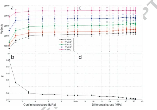
332
During the isotropic loading (Phase 0), and for all propagation
direc-333
tions, a significant increase in Vp with a confining pressure increase from
334
0 to 3 MPa is observed, with only slight increase between 3 and 10 MPa
335
(Fig. 7a). Despite the uncertainty in the estimation of the absolute value
336
of Vp (the worst case scenario is represented by the error bars in Fig. 7a),
337
the relative magnitudes of Vp along the different propagation directions can
338
be considered as reliable. The elastic anisotropy of the shale is clearly
high-339
lighted, with a slow Vp(90◦) and a fast Vp(0◦) velocity across and along the 340
bedding, respectively. We also observe that Vp(60◦), Vp(45◦) and Vp(30◦) 341
exhibit intermediate values, inversely proportional to their angular
inclina-342
tion with respect to the bedding plane. This suggests that the shale specimen
343
can reasonably be assumed to be transversely isotropic (TI) in terms of its
344
dynamic elastic response. This phenomenon has also been extensively
re-345
ported in the literature for many shales of different origin and geological
346
history (e.g., [40, 41] and references therein)
In view of the size of the ultrasonic transducers and the propagation
348
distances within the specimen, the estimated P-wave velocities are assumed
349
to be group (ray) velocities ([12]). However, along the symmetry axis and
350
the symmetry plane of the TI shale, group (ray) and phase velocity coincide.
351
Therefore, Thomsen’s parameter [47] ε = (Vp(0◦)2 - Vp(90◦)2)/2Vp(90◦)2 352
quantifying the P-wave anisotropy in a TI medium can be estimated using
353
the measured group velocities (Fig. 7b, d).
354
The P-wave velocity and the corresponding P-wave anisotropy as
mea-355
sured by Thomsen’s ε parameter exhibit a significant dependency to the
356
confining pressure (Fig. 7a, b): εdrops from 1.8 to 0.8 between 0 and 3 MPa
357
and remains almost constant from 3 to 10 MPa. This suggests a closure
358
of pre-existing micro-cracks (damage) sub-parallel to the bedding with the
359
increase in effective pressure, which is consistent with the dependency of the
360
gas permeability to effective pressure reported in Section 2.1. In contrast,
361
during the deviatoric stress loading (Phases 1 to 3), P-wave velocities appear
362
nearly constant or rise slightly (Fig. 7c), and Thomsen’s parameter ε exhibits
363
a moderate dependency to deviatoric stress (Fig. 7d), decreasing to 0.6 as
364
differential stress increases from 0 to 35 MPa.
365
4.2. P-wave velocity model of the shale sample
366
In order to spatially locate the MSEs recorded during the experiment,
367
a P-wave velocity model is required. Based on the analysis of the P-wave
368
velocity data, the velocity model should in principle account for the TI nature
369
of the elastic properties of the shale and the variation of the P-wave velocities
370
with stress. However, as the aim is only to locate MSEs recorded during the
371
deviatoric stress loading (Phases 1 to 3), and accounting for the fact that the
P-wave velocities are not significantly affected by the deviatoric stress during
373
these phases (Fig. 7c and d), the velocities recorded at the start of Phase
374
1 are used to build the required velocity model of the shale, that is when
375
the confining pressure is 10 MPa and the axial stress is zero. Note that this
376
model is only a pragmatic approximation assuming that the shale specimen
377
is homogeneous.
378
In addition, because their spatial location is known, the ultrasonic sources
379
shot during the velocity surveys can first be used to assess the validity of both
380
the location (inversion) algorithm and the selected TI velocity model. A
381
Simplex algorithm implemented in the Insite software, and a velocity model
382
based on a slow velocity Vp(90◦) = 2000 m/s and an ε = 0.78 are used. The 383
orientation of the symmetry axis of this model is inferred from the known
384
orientation of the bedding in the specimen, that is at 45◦ to the specimen’s 385
axis.
386
Although this velocity model accounts for the experimentally estimated
387
velocity and anisotropy, at the scale of the specimen used in this experiment,
388
this combination of values produced a distorted pattern of location of the
389
source shots. In an attempt to improve the results and optimise the
proce-390
dure, several values of the slow velocity Vp(90◦) and the value of ε are tested. 391
The combination that produces the best source shots locations is found to be
392
Vp(90◦) = 1900 m/s and ε = 0.625. Because the velocity field is not strongly 393
affected by the axial load and related displacement during Phases 1 to 3 (see
394
Fig. 7c), we use this velocity field for all source shots location and MSEs
395
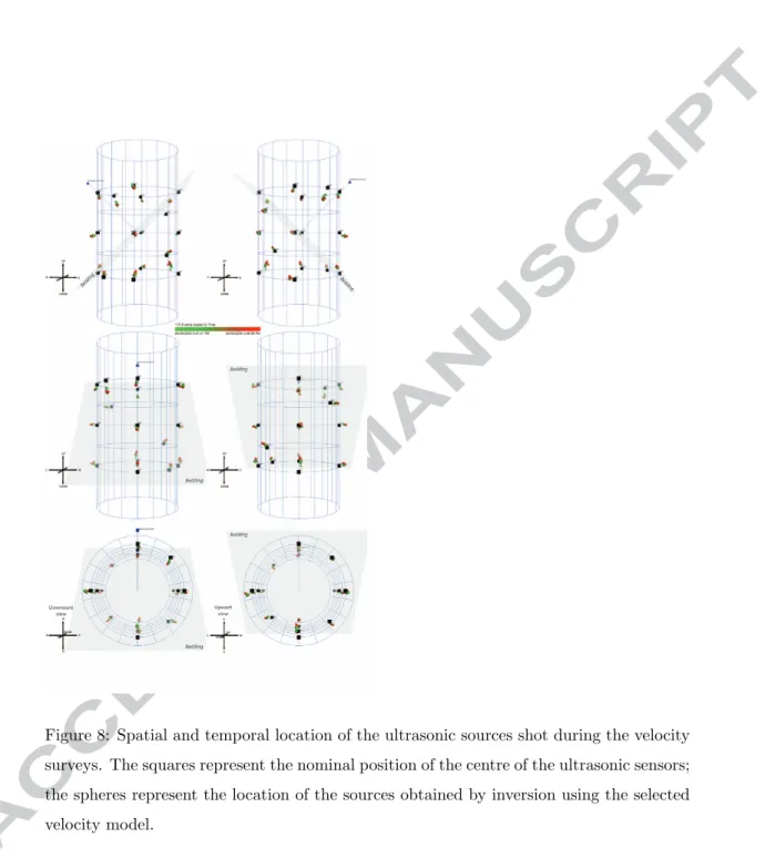
recorded during these phases. The inversion using these values and applied
396
to 176 ultrasonic shots (for all the velocity surveys conducted during Phases
1 to 3) reflects reasonably well the known position of the ultrasonic array,
398
i.e. the sources clearly locate in the vicinity of the transducers (Fig.8). The
399
uncertainty associated specifically with the location of these source shots for
400
all surveys conducted during Phases 1 to 3 amounts to 0.9 mm in average
401
for an average number of triggered sensors of 12. This residual mismatch
402
between the recovered and the actual sensor positions can reasonably be
at-403
tributed to: (i) the progressive loss of transverse isotropy of the shale during
404
the application of the deviatoric stress (not aligned with the original
sym-405
metry axis); (ii) the natural and stress induced heterogeneity of the velocity
406
field in the shale specimen (including the effects of shear fracturing/faulting);
407
and (iii) the relative motion of the sensors during the shear fracturing and
408
faulting in Phases 2 and 3. The pragmatic selection of the adequate velocity
409
structure (Vp(90◦) = 1900 m/s and ε = 0.625) partially compensates for 410
these uncertainties in view of the results of the source shots location (Fig.8).
411
4.3. Analysis of the induced micro-seismicity
412
4.3.1. Spatio-temporal evolution
413
According to the passive monitoring protocol described in Section 2.3,
414
nearly 500 events are detected during the whole experiment, although not
415
all of them are identified as MSEs. Due to the reasonable number of events
416
recorded, a manual check of the acquired data set was possible. A number
417
of events are identified as electronic noise while others are discarded due to
418
the low SNR of the recorded waveforms. Finally, only the events that could
419
be reliably located within the volume of the specimen are selected for further
420
analysis (Fig. 9). This procedure finally leads to the selection of a total of 280
421
MSEs: 34 during Phase 1 (yellow spheres in Fig. 9), 14 during Phase 2 (blue
spheres), and 232 during Phase 3 (pink spheres). The average location error
423
for the whole dataset is 2.3 mm for an average number of triggered sensors
424
of 12. This location error is computed for each MSE during the inversion
425
based on the residuals and knowing the velocity structure of the medium.
426
The causes of this uncertainty are related to the experimental uncertainties
427
in the determination of the exact position of the sensors, the heterogeneity
428
of the rock sample, the uncertainty associated with the determination of
429
the (homogeneous but anisotropic) velocity structure to match the actual
430
velocity along the various ray paths. For an imposed axial displacement of
431
1 mm/hour (Phase 2), the average rate of MSEs is 0.07 MSE/second. This
432
value reaches an average of 0.19 MSE/second over the whole Phase 3 of
433
imposed axial displacement at 10 mm/hour.
434
Only 64 events are detected during Phase 0 of confining pressure loading
435
applied to reach the simulated in situ stress. Out of these events, 15 MSEs
436
with sufficient SNR have been identified and spatially localised. They were
437
randomly located in the volume of the shale specimen. For sake of clarity
438
and because they are not induced by the triaxial loading, these events have
439
been discarded and are not represented in Fig. 9.
440
The spatial distribution of the MSEs is clearly not random: they appear
441
distributed along two main planar structures, sub-parallel to the shale
bed-442
ding (Fig. 10). A first structure, highlighted as a yellow plane, is initiated
443
during Phase 1: few yellow MSEs seem to be distributed over the volume
444
of the specimen, but most of them appear to cluster along the highlighted
445
yellow plane. This reflects an initial diffuse damage, then a first pattern of
446
strain localisation in the vicinity of the yellow plane. The second structure,
highlighted as a pink plane, is initiated during Phase 2 (slow slip, blue MSEs)
448
and largely develops during Phase 3 (fast slip, pink MSEs). Note however
449
that the MSEs occurring during Phase 3 do not locate only in the vicinity
450
of the pink plane, but also in the overlap volume between the yellow and
451
pink planes, and on the yellow plane to a lesser extent. In addition, there
452
are few yellow MSEs located on the pink plane, which suggests that shear
453
faulting could have been initiated simultaneously on both planes, then the
454
upper shear plane takes over the lower one and accommodates most of the
455
rock shortening at the end of the experiment.
456
The above results are derived from the combined use of active ultrasonic
457
and passive MS monitoring of the deformation process. Both monitoring
458
techniques are based only on the picking of the time of arrival of the first
459
phase in the recorded waveforms.
460
4.3.2. Moment tensor analysis
461
The first motion polarities and relative amplitudes of the waveforms
462
recorded for a given MSE can be used to estimate its source mechanism,
463
similar to the approach widely used in seismology to define the source
mech-464
anism of earthquakes. This method, generally known as the Moment Tensor
465
Inversion (MTI), is implemented in the Insite software and is used here to
466
characterise the focal mechanism of the recorded MSEs [37, 52, 53, 54].
How-467
ever, in order to obtain reliable MTI results, the analysis must be restricted
468
to MSEs of sufficiently high quality, which represent a relatively small subset
469
of all the spatially located MSEs. The MTI has been carried out on all the
470
MSEs located spatially. The results reported Figure 10 fulfil the additional
471
criteria: (i) a spatial location error strictly lower than 5 mm; (ii) a mean
error factor lower than 17; (iii) an inversion quality index lower than 4.4;
473
and (iii) a T-k error norm lower than 0.3. The mean error factor measures
474
the difference between the amplitude residual and the estimated uncertainty
475
in the original amplitude measurement. The inversion quality factor is based
476
on the 6x6 covariance matrix and depends on the Green’s functions used,
477
rather than the amplitudes. It is computed from the sum of the squares of
478
the elements of the covariance matrix. The T-k error norm is the RMSE of
479
the errors on the deviatoric (T) and isotropic (k) parameters representing the
480
source [23]. The threshold values of the mean error factor, inversion quality
481
index and T-k error norm have been selected as the mean values obtained for
482
the whole set of spatially located MSEs to which the MTI has been carried
483
out. With such criteria, 42 MSEs have been selected: 11 MSEs in Phase
484
1, 6 MSEs in Phase 2 and 25 in Phase 3. The average amplitude residual
485
parameter for these 42 MSEs is 0.21, and the standard deviation is 0.08.
486
Figure 11 shows the spatial distribution of the 42 MSEs within the shale
487
specimen. For each MSE, the detecting ultrasonic sensors covered a
reason-488
able portion of the solid angle around it, which allowed for a reliable MTI. In
489
this figure, MSEs #79 in Phase 1, #128 in Phase 2 and #259 in Phase 3 have
490
been highlighted because they exhibit the largest location magnitude for each
491
phase. For each of these three MSEs, the focal mechanism is represented by a
492
focal sphere plot, i.e., the so-called beachballs widely used in seismology. The
493
sensors that detected the MSE are represented by small discs in the
beach-494
balls, with the convention that black and white discs represent compressional
495
and dilatational first motion, respectively. The fault plane is calculated using
496
the first-motion polarity of the P-wave picked in the waveform recorded by
each sensor that detected this MSE and is represented by red circles in each
498
focal sphere plot. The orientation of the fault plane is consistent with that of
499
the fault planes identified statistically by the spatial distribtion of the MSEs
500
and by the post-mortem observation of the sample.
501
The MTI procedure yields the focal mechanism of each MSE as a
combi-502
nation of three basic modes, with usually a dominant mode: ISO, stands for
503
isotropic dilatation, DC for double-couple (shear), and CLVD for
compen-504
sated linear vector dipole [44, 52]. Hudson’s so-called T-k source-type plot
505
([23]) is well-suited to display such decomposition in an equal-area graph
506
(Fig. 11) where the T stands for the deviatoric component of the
mech-507
anism (shear deformation, zero volume change) and k stands for the
nor-508
mal/isotropic component (volumetric deformation, either positive-explosive
509
or negative-implosive).
510
Figure 12 reports graphically the results of the moment tensor
decom-511
position of the selected high quality MSEs. Figure 12a shows the detailed
512
decomposition of the focal mechanisms into Hudson’s T-k source types;
fig-513
ure 12b shows the corresponding decomposition into DC, CLVD and ISO
514
MSEs; figure 12c shows the corresponding decomposition into pure shear
515
(DC) and non-shear (ISO+CLVD) MSEs; and figure 12d represents the fault
516
plane orientation for the selected MSEs in terms of azimuth and dip angles.
517
In each of these plots, the raw data as obtained through the moment tensor
518
inversion are represented with coloured symbols; the corresponding coloured
519
lines are obtained by a moving average procedure with a window size of 9
520
points. The purpose of these lines is only to identify possible trends during
521
the three phases of the experiment. The T-k decomposition suggests that
at the early stages of Phase 1, damage is dominated by non-shear MSEs (k
523
or ISO+CLVD MSEs). A transition toward more shear MSEs occurs during
524
Phases 2 and 3 (Fig. 12a and c). During most of Phase 3, the most common
525
mechanisms is double couple, and by the end of the experiment, all
mech-526
anisms (DC, CLVD and ISO) become equiprobable (Fig. 12b). Figure 12d
527
suggests that the most probable dip angle of the fault plane is comprised
528
between 30 and 60; the most probable azimuth angle is comprised between
529
120 and 180. These angles are qualitatively consistent with the macroscopic
530
shear fractures observed on the rock specimen post-mortem. The variability
531
of the dip and azimuth angles around their nominal values of 45 and 180 can
532
be attributed to the experimental uncertainties associated with the
measure-533
ments and the inversion procedure. They could also be related to the shear
534
failure of small asperities on the fault plane that are not well aligned with
535
the macroscopic failure plane (see discussion below).
536
5. Discussion
537
5.1. Shear faulting in the laboratory and relay ramp structures in the field
538
The post-mortem picture of the failed specimen and the location of the
539
recorded MSEs are in good agreement (see Fig. 10). Although the picture
540
of the specimen cannot show the internal structure of the shear faults, their
541
emergence at the external boundary of the specimen is in agreement with the
542
location of the MSEs at this boundary. Two different planar structures are
543
identified from the spatio-temporal location of the 280 MSEs (Figs. 9 and
544
10).
545
These results suggest that the lower shear fault (yellow plane) is most
active (accommodates most of the imposed axial dis- placement) at the early
547
stages after strain localisation (Phase 1), although few yellow events are
548
already located on the top part of the upper shear fault. However, during
549
this phase no clustering of MSE is observed on this upper plane. During
550
Phase 2, a transition of the micro-seismic activity is observed from the lower
551
shear fault toward the upper shear fault (pink plane). During Phase 3 most
552
of the imposed axial displacement is accommodated by the upper shear fault,
553
although few events are still located on the lower shear fault, indicating that
554
it is not entirely inactive. This is consistent with the sequence of events
555
associated with a typical relay ramp structure formed during the growth of
556
normal fault systems in large scale geology
557
This upward transition from the lower to the upper SF is particularly
558
visible in Figure 10 where the MSEs in each phase have been colour-coded
559
according to their time of occurrence within the phase. More precisely, once
560
the yellow SF is formed and its activity slows down at the end of Phase
561
1, the blue MSEs of Phase 2 first appear at the lower end of the pink SF
562
then the MS activity migrates upward along this SF and approaches the
563
boundary of the specimen. Once the pink SF is largely developed, part of
564
the MS activity (pink MSEs) locates in the overlap volume between the two
565
SF planes. In summary, it seems that the lower shear fault forms first (yellow
566
plane), before the micro-seismic activity (blue spheres) migrates upward and
567
the upper shear fault forms and accommodates most of the subsequently
568
imposed axial displacement (pink plane). This is essentially similar to typical
569
sequence of events associated with either (i) the formation of a relay ramp
570
structure during the growth of normal fault systems in large scale geology;
or (ii) fractures growing towards one another and overlapping.
572
5.2. Silent failure, slow slip and slip rate dependency
573
Phase 1 is quasi-aseismic (only 34 MSEs), at least in the 0.5 MHz range
574
of sensitivity of the ultrasonic transducers used in the experiment (about 0.1
575
to 1 MHz). This is surprising because Phase 1 corresponds to the failure of
576
the clay-rich rock and contrasts with other sedimentary or crystalline rocks
577
(e.g., sandstones, granites) for which large amounts of precursory MSEs are
578
usually recorded prior to the macroscopic failure, and failure itself has been
579
reported to generate a much stronger MS activity (thousands of events).
580
Phase 2 of slow slip on the yellow shear fault induces very small amount of
581
MS activity: clays might be acting as a lubricant on the fault(s) at that slip
582
rate. Silent or almost silent failures have already been reported in materials
583
being deformed close to the brittle ductile transition, for instance Carrara
584
marble [43], or Volterra gypsum at room temperature [5]. In all cases, silent
585
failures are accompanied by slow slip and stress drop, i.e. the macroscopic
586
fault releases the stress too slowly for the rupture and the slip to accelerate
587
and start radiating elastic waves. As such, slow failures can be viewed as
588
quasi-static failures in the Griffith sense, i.e., the entire energy release rate is
589
dissipated at the rupture tip into fracture surface, damage and plastic strain.
590
Note that slow failures are not always silent, because at the microscopic
591
scale, damage at the crack tip can actually also radiate elastic waves and be
592
associated to MSEs, as for instance during quasi static fault growth in granite
593
[33], slow failure in porous basalt [4] or shear or compaction band formation
594
in sandstones [15, 17]. Hence, both the growth of macroscopic fracture and
595
the accumulation of microscopic damage are silent in the frequency range
investigated in these experiments. This suggests that shale and clays are
597
indeed potential good candidate to host slow slip within shallow accretionary
598
prism [19, 22], or in the shallow section of continental faults [50].
599
In contrast, Phase 3 of slip acceleration from 1mm/h to 10mm/h, i.e.
600
slip slip velocities slightly larger than that observed during slow earthquakes
601
which are typically of the order of several tens of cm per year only [20],
602
generates a significant amount of MS activity. During that fast slip phase,
603
the AE rate and the slip are proportional so there seems to be a
signifi-604
cant rate dependency of the lubrication potential of clays. In Figure 13, we
605
can see that the slip acceleration triggers an instantaneous increase in the
606
friction coefficient, which is typical of the direct effect [35]. After that, the
607
fault first weakens with increasing slip, then starts to re-strengthen after a
608
few millimetres of slip, exhibiting thus the typical velocity strengthening
be-609
haviour observed for clay minerals [38]. It is interesting to note that during
610
that phase, nevertheless, numerous MSEs are observed, probably linked to
611
the dynamic shear failure of small asperities on the fault plane, as
demon-612
strated by the inverted focal mechanisms (see Fig 13). These observations
613
highlight the possible interactions between small asperities and slow slip of
614
a velocity-strengthening fault [3], which could be considered as a realistic
615
experimental analogue of natural observations of non-volcanic tremors and
616
(very) low-frequency earthquakes triggered by slow slip events [19, 21].
617
6. Conclusion
618
We have demonstrated that it is possible to apply laboratory techniques
619
usually employed for monitoring micro-seismicity on reservoir or crystalline
rocks to anisotropic shale specimens. The data acquired during this triaxial
621
experiment allowed us (i) to quantify the P-wave (dynamic) anisotropy of
622
the shale and its evolution with stress; (ii) monitor the micro-seismic
activ-623
ity occurring during failure and subsequent fault slip at two different rates.
624
The gas permeability as well as the P-wave velocity data and their respective
625
sensitivity to pressure suggest the existence of micro-cracks in this partially
626
dry shale specimen at room conditions. Although these micro-cracks tend to
627
close with increasing effective confining pressure. The spatio-temporal
loca-628
tion of the MSEs recorded during the three phases of the experiment (failure,
629
slow fault slip, fast fault slip) indicates that two shear fault planes where in
630
competition after the initial strain localisation that occurred near the peak
631
axial stress. The evolution of these two shear fault planes as derived from the
632
micro-seismic monitoring is consistent with the sequence of events associated
633
with a typical relay ramp structure formed during the growth of normal fault
634
systems in large scale geology. The moment tensor inversion carried out on
635
the highest quality MSEs suggests a transition form non-shear dominated
636
to shear-dominated micro-seismic activity when the rock evolves from initial
637
failure to larger and faster slip along the fault. The spatial orientation of the
638
fault plane obtained on the highest magnitude MSE for each phase is
con-639
sistent with the macroscopic orientation of the shear faults. The frictional
640
behaviour of the shear faults highlights the possible interactions between
641
small asperities and slow slip of a velocity-strengthening fault, which could
642
be considered as a realistic experimental analogue of natural observations of
643
non-volcanic tremors and (very) low-frequency earthquakes triggered by slow
644
slip events.
Acknowledgments
646
This research work was sponsored by BP under the contract number
647
BPO-06-01329. This support is gratefully acknowledged.
References
649
[1] Amitrano D., Brittle-ductile transition and associated seismicity:
650
Experimental and numerical studies and relationship with the
651
b value, Journal of Geophysical Research-Solid Earth, 108(B1),
652
doi:10.1029/2001JB000680, 2003.
653
[2] Amann F., Button E.A., Evans K.F., Gischig V.S., and Bl¨umel M.,
Ex-654
perimental study of the brittle behavior of clay shale in rapid unconfined
655
compression, Rock Mechanics and Rock Engineering, 44, 415 - 430, 2011.
656
[3] Ariyoshi K., Hori T., Ampuero J.P., Kaneda Y., Matsuzawa T., Hino R.
657
and Hasegawa A., Influence of interaction between small asperities on
658
various types of slow earthquakes in a 3-D simulation for a subduction
659
plate boundary, Gondwana Research, 16, 534 - 544, 2009.
660
[4] Benson P.M., Thompson B.D., Meredith P.G., Vinciguerra S. and Young
661
R.P., Imaging slow failure in triaxially deformed Etna basalt using 3D
662
acoustic?emission location and X?ray computed tomography,
Geophys-663
ical Research Letters, 34(3), 2007.
664
[5] Brantut N., Schubnel A. and Gu´eguen Y., Damage and rupture
dynam-665
ics at the brittle?ductile transition: The case of gypsum, Journal of
666
Geophysical Research-Solid Earth, 116(B1), 1978 - 2012, 2011.
667
[6] Chang S.-H., and Lee C.-I., Estimation of cracking and damage
mecha-668
nisms in rock under triaxial compression by moment tensor analysis of
669
acoustic emission, International Journal of Rock mechanics and Mining
670
Sciences, 41, 1069 - 1086, 2004.
[7] Charalampidou E.-M., Hall S.A., Stanchits S., Lewis H., and Viggiani
672
G., Characterization of shear and compaction bands in a porous
sand-673
stone deformed under triaxial compression, Tectonophysics, 503, 8 - 17,
674
2011.
675
[8] Charalampidou E.-M., Stanchits S., Kwiatek G., and Dresen G., Brittle
676
failure and fracture reactivation in sandstone by fluid injection, European
677
Journal of Environmental and Civil Engineering, 19, 564 - 579, 2015.
678
[9] Dautriat J., Sarout J., David C., Bertauld D., and Macault R., Remote
679
monitoring of the mechanical instability induced by fluid substitution
680
and water weakening in the laboratory, Physics of the Earth and
Plan-681
etary Interiors, This issue.
682
[10] David C., Dautriat D., Sarout J., Delle Piane C., Men´endez B., Macault
683
R., and Bertauld D., Mechanical instability induced by water weakening
684
in laboratory fluid injection tests, Journal of Geophysical Research-Solid
685
Earth, 120, 4171 - 4188, doi:10.1002/ 2015JB011894.
686
[11] Delle Piane C., Dewhurst D.N., Siggins A.F. and Raven M.,
Stress-687
induced anisotropy in brine saturated shale, Geophysical Journal
Inter-688
national, 184, 897 - 906, 2011.
689
[12] Dellinger J., and Vernik L., Do travel times in pulse transmission
ex-690
periments yield anisotropic group or phase velocities?, Geophysics, 41,
691
1774 - 1779, 1994.
692
[13] Dewhurst D.N. and Siggins A.F., Impact of fabric, microcracks and
stress field on shale anisotropy, Geophysical Journal International, 165,
694
135 - 148, 2006.
695
[14] Dewhurst D.N., Siggins A.F., Sarout J. and Raven M., Geomechanical
696
and ultrasonic characterization of a Norwegian Sea shale, Geophysics,
697
76, WA101 - WA111, 2011.
698
[15] Fortin J., Stanchits S., Dresen G., and Gueguen Y., Acoustic emission
699
and velocities associated with the formation of compaction bands in
700
sandstone, Journal of Geophysical Research-Solid Earth, 111, B10203,
701
doi:10.1029/2005JB003854, 2006.
702
[16] Fortin J., Stanchits S., Dresen G., and Gueguen Y., Damage evolution,
703
acoustic emissions and elastic wave velocities in porous carbonate rocks,
704
AGU Fall Meeting Abstracts, #T23D-0539, 2009.
705
[17] Fortin J., Stanchits S., Dresen G., and Gueguen Y., Acoustic emissions
706
monitoring during inelastic deformation of porous sandstone:
Compar-707
ison of three modes of deformation, Pure and Applied Geophysics, 166,
708
823 - 841, 2009.
709
[18] Guglielmi Y., Cappa F., Avouac J.-P., Henry P., and Elsworth D.,
Seis-710
micity triggered by fluid injection-induced aseismic slip, Science, 348,
711
1224 - 1226, 2015.
712
[19] Hirose H., Asano Y., Obara K., Kimura T., Matsuzawa T., Tanaka S.
713
and Maeda T., Slow earthquakes linked along dip in the Nankai
subduc-714
tion zone, Science, 330, 1502 - 1502, 2010.
[20] Ikari M.J., Ito Y., Ujiie K. and Knopf A.J., Spectrum of slip behaviour
716
in Tohoku fault zone samples at plate tectonic slip rates, Nature
Geo-717
sciences, 2015.
718
[21] Ito Y., Obara K., Shiomi K., Sekine S. and Hirose H., Slow earthquakes
719
coincident with episodic tremors and slow slip events, Science, 315, 503
720
- 506, 207.
721
[22] Ito Y., Hino R., Kido M., Fujimoto H., Osada Y., Inazu D. and Mishina
722
M., Episodic slow slip events in the Japan subduction zone before the
723
2011 Tohoku-Oki earthquake, Tectonophysics, 600, 14 - 26, 2013.
724
[23] Hudson J.A., Pearce R.G. and Rogers R.M., Source type plot for
inver-725
sion of the moment tensor, Journal of Geophysical Research-Solid Earth,
726
91, 765 - 774, 1989.
727
[24] Johnston J.E. and Christensen N.I., Seismic anisotropy of shales,
Jour-728
nal of Geophysical Research-Solid Earth, 100(B4, 5991 - 6003, 1995.
729
[25] Josh M., Esteban L., Delle Piane C., Sarout J., Dewhurst D.N. and
730
Clennell M.B., Laboratory characterisation of shale properties, Journal
731
of Petroleum Science and Engineering, 88-89, 107 - 124, 2012.
732
[26] Kusunose K., Lei X., Nishizawa O. and Satoh T., Effect of grain size on
733
fractal structure of acoustic emission hypocenter distribution in granitic
734
rock, Physics of the Earth and Planetary Interiors, 67, 194 - 199, 1991.
735
[27] Le Gonidec Y., Sarout J., Wassermann J. and Nussbaum C.,
Dam-736
age initiation and propagation assessed from stress-induced microseismic
events during a mine-by test in the Opalinus Clay, Geophysical Journal
738
International, 198, 126 - 139, 2014.
739
[28] Lei X., Kusunose K., Satoh T. and Nishizawa O., The hierarchical
rup-740
ture process of a fault: an experimental study, Physics of the Earth and
741
Planetary Interiors, 137, 213 - 228, 2003.
742
[29] Lei X., Masuda K., Nishizawa O., Jouniaux L., Liu L., Ma W., Satoh T.
743
and Kusunose K., Detailed analysis of acoustic emission activity during
744
catastrophic fracture of faults in rock, Journal of Structural Geology,
745
26, 247 - 258, 2004.
746
[30] Lei X., Nishizawa O., Kusunose K., Cho A., Satoh T. and Nishizawa O.,
747
Compressive failure of mudstone samples containing quartz veins using
748
rapid AE monitoring: the role of asperities, Tectonophysics, 328, 329
-749
340, 2000.
750
[31] Lei X. and Satoh T., Indicators of critical point behavior prior to rock
751
failure inferred from pre-failure damage, Tectonophysics, 431, 97 - 111,
752
2007.
753
[32] Lockner D.A., The role of acoustic emission in the study of rock fracture,
754
International Journal of Rock Mechanics and Mining Sciences, 30, 883
755
- 899, 1993.
756
[33] Lockner D.A., Byerlee J.D., Kuksenko V., Ponomarev A. and Sidorin A.,
757
Quasi-static fault growth and shear fracture energy in granite, Nature,
758
350, 39 - 42, 1991.
[34] Lowry A.R., Larson K.M., Kostoglodov V. and Bilham R., Transient
760
fault slip in Guerrero, southern Mexico, Geophysical Research Letters,
761
28, 3753 - 3756, 2001.
762
[35] Marone C., Laboratory-derived friction laws and their application to
763
seismic faulting, Annual Review of Earth and Planetary Sciences, 26,
764
643 - 696, 1998.
765
[36] Niemeijer A.R. and Spiers C.J., Influence of phyllosilicates on fault
766
strength in the brittle-ductile transition: insights from rock analogue
767
experiments, Special publication-Geological Society of London, 245, 303,
768
2005.
769
[37] Pettitt W.S., Baker C., Young R.P., Dahlstrm L.-O. and Ramqvist G.,
770
The assessment of damage around critical engineering structures using
771
induced seismicity and ultrasonic techniques, Pure and Applied
Geo-772
physics, 159, 179 - 195, 2002.
773
[38] Safer D.M. and Marone C., Comparison of smectite-and illite-rich gouge
774
frictional properties: application to the updip limit of the seismogenic
775
zone along subduction megathrusts, Earth and Planetary Science
Let-776
ters, 215, 219 - 235, 2003.
777
[39] Sarout J., Delle Piane C., Nadri D., Esteban L. and Dewhurst D.N.,
778
A robust experimental determination of Thomsen’s δ parameter,
Geo-779
physics, 80, A19 - A24, 2015.
780
[40] Sarout J., Esteban L., Delle Piane C., Maney B. and Dewhurst D.N.,