HAL Id: hal-00317125
https://hal.archives-ouvertes.fr/hal-00317125
Submitted on 1 Jan 2003
HAL is a multi-disciplinary open access
archive for the deposit and dissemination of
sci-entific research documents, whether they are
pub-lished or not. The documents may come from
teaching and research institutions in France or
abroad, or from public or private research centers.
L’archive ouverte pluridisciplinaire HAL, est
destinée au dépôt et à la diffusion de documents
scientifiques de niveau recherche, publiés ou non,
émanant des établissements d’enseignement et de
recherche français ou étrangers, des laboratoires
publics ou privés.
New method in computer simulations of electron and
ion densities and temperatures in the plasmasphere and
low-latitude ionosphere
A. V. Pavlov
To cite this version:
A. V. Pavlov. New method in computer simulations of electron and ion densities and temperatures in
the plasmasphere and low-latitude ionosphere. Annales Geophysicae, European Geosciences Union,
2003, 21 (7), pp.1601-1628. �hal-00317125�
Annales Geophysicae (2003) 21: 1601–1628 c European Geosciences Union 2003
Annales
Geophysicae
New method in computer simulations of electron and ion densities
and temperatures in the plasmasphere and low-latitude ionosphere
A. V. PavlovInstitute of Terrestrial Magnetism, Ionosphere and Radio-Wave Propagation, Russia Academy of Science (IZMIRAN), Troitsk, Moscow Region, 142190, Russia
Received: 23 August 2002 – Revised: 16 January 2003 – Accepted: 15 February 2003
Abstract. A new theoretical model of the Earth’s low- and mid-latitude ionosphere and plasmasphere has been devel-oped. The new model uses a new method in ionospheric and plasmaspheric simulations which is a combination of the Eu-lerian and Lagrangian approaches in model simulations. The electron and ion continuity and energy equations are solved in a Lagrangian frame of reference which moves with an in-dividual parcel of plasma with the local plasma drift velocity perpendicular to the magnetic and electric fields. As a re-sult, only the time-dependent, one-dimension electron and ion continuity and energy equations are solved in this La-grangian frame of reference. The new method makes use of an Eulerian computational grid which is fixed in space co-ordinates and chooses the set of the plasma parcels at every time step, so that all the plasma parcels arrive at points which are located between grid lines of the regularly spaced Eule-rian computational grid at the next time step. The solution values of electron and ion densities Neand Ni and temper-atures Te and Ti at the Eulerian computational grid are ob-tained by interpolation. Equations which determine the tra-jectory of the ionospheric plasma perpendicular to magnetic field lines and take into account that magnetic field lines are “frozen” in the ionospheric plasma are derived and included in the new model.
We have presented a comparison between the modeled
NmF2 and hmF2 and NmF2 and hmF2 which were observed
at the anomaly crest and close to the geomagnetic equator simultaneously by the Huancayo, Chiclayo, Talara, Bogota, Panama, and Puerto Rico ionospheric sounders during the 7 October 1957 geomagnetically quiet time period at solar maximum. The model calculations show that there is a need to revise the model local time dependence of the equatorial upward E × B drift velocity given by Scherliess and Fe-jer (1999) at solar maximum during quiet daytime equinox conditions. Uncertainties in the calculated Ni, Ne, Te, and
Ti resulting from the difference between the NRLMSISE-00 and MSIS-86 neutral temperatures and densities and from
Correspondence to: A. V. Pavlov (pavlov@izmiran.rssi.ru)
the difference between the EUV97 and EUVAC solar fluxes are evaluated. The decrease in the NRLMSISE-00 model [O]/[N2] ratio by a factor of 1.7–2.1 from 16:12 UT to 23:12 UT on 7 October brings the modeled and measured
NmF2 and hmF2 into satisfactory agreement. It is shown that
the daytime peak values in Te, and Ti above the ionosonde stations result from the daytime peak in the neutral tem-perature. Our calculations show that the value of Te at F2-region altitudes becomes almost independent of the electron heat flow along the magnetic field line above the Huancayo, Chiclayo, and Talara ionosonde stations, because the near-horizontal magnetic field inhibits the heat flow of electrons. The increase in geomagnetic latitude leads to the increase in the effects of the electron heat flow along the magnetic field line on Te. It is found that at sunrise, there is a rapid heat-ing of the ambient electrons by photoelectrons and the differ-ence between the electron and neutral temperatures could be increased because nighttime electron densities are less than those by day, and the electron cooling during morning con-ditions is less than that by day. This expands the altitude region at which the ion temperature is less than the electron temperature near the equator and leads to the sunrise electron temperature peaks at hmF2 altitudes above the ionosonde sta-tions. After the abrupt increase at sunrise, the value of Te de-creases, owing to the increasing electron density due to the increase in the cooling rate of thermal electrons and due to the decrease in the relative role of the electron heat flow along the magnetic field line in comparison with cooling of ther-mal electrons. These physical processes lead to the creation of sunrise electron temperature peaks which are calculated above the ionosonde stations at hmF2 altitudes. We found that the main cooling rates of thermal electrons are electron-ion Coulomb colliselectron-ions, vibratelectron-ional excitatelectron-ion of N2and O2, and rotational excitation of N2. It is shown that the increase in the loss rate of O+(4S) ions due to the vibrational excited N2and O2leads to the decrease in the calculated NmF2 by a factor of 1.06–1.44 and to the increase in the calculated
hmF2, up to the maximum value of 32 km in the low-latitude
lati-1602 A. V. Pavlov: New method in computer simulations of electron and ion densities and temperatures tude. Inclusion of vibrationally excited N2and O2brings the
model and data into better agreement.
Key words. Ionosphere (equatorial ionosphere; electric fields and currents, plasma temperature and density; ion chemistry and composition; ionosphere-atmosphere interac-tions; modeling and forecasting)
1 Introduction
At low- and mid-latitudes, the Earth’s magnetic field can be represented, to a good approximation, by a dipole. The horizontal orientation of the geomagnetic field at the ge-omagnetic equator is known to be the basic reason for the active nature of the low-latitude ionosphere, which is characterised by the equatorial electrojet, equatorial plasma fountain, equatorial (Appleton) anomaly, additional layers, plasma bubbles, and spread-F. These equatorial character-istic properties of the ionosphere have been studied obser-vationally and theoretically for many years (see, for exam-ple, review papers presented by Moffett, 1979; Anderson, 1981; Walker, 1981; Rishbeth, 2000; Abdu, 1997, 2001, and references therein). Many theoretical models of the plasmasphere and low-latitude ionosphere were constructed and have been applied to study a wide variety of equato-rial ionosphere characteristic properties. Among these mod-els, it is necessary to point out the following major so-phisticated plasmaspheric and low-latitude ionospheric mod-els: the Sheffeld University plasmasphere-ionosphere model (Bailey and Sellec, 1990; Bailey and Balan, 1996), the cou-pled thermosphere-ionosphere-plasmasphere model (CTIP) (Fuller-Rowell et al., 1988; Millward et al., 1996), a coupled thermosphere-ionosphere model (CTIM) (Fuller-Rowell et al., 1996), the global theoretical ionospheric model (GTIM) (Anderson, 1973; Anderson et al., 1996), and the global numerical self-consistent and time-dependent model of the thermosphere, ionosphere, and protonosphere (Namgaladze et al., 1988). These models include transport of plasma by geomagnetic field-aligned diffusion and neutral wind-induced plasma drift of ions and electrons, and plasma mo-tion perpendicular to the geomagnetic field, B, due to an electric field, E, which is generated in the E-region. This electric field affects F-region plasma causing both ions and electrons to drift in the same direction with an drift velocity,
VE=E × B/B2.
In a Lagrangian method, the finite-difference grid moves with the local plasma drift velocity VEperpendicular to the magnetic and electric fields. The rate of change of elec-tron and ion number densities and temperatures in a mov-ing frame of reference is much easier to compute because the convective terms in the continuity and energy equations are absent in the moving frame. As a result, it is needed to solve only one-dimensional, time dependent ion and electron continuity and energy equations along magnetic field lines in this moving frame of reference.
Contrary to a Lagrangian computational grid, an Eulerian computational grid is fixed in space coordinates. The main aim of our work is to elaborate a new approach which in-cludes the advantages of both approaches in solving electron and ion continuity and energy equations in the ionosphere and plasmasphere. Our new approach is a combination of the Eulerian and Lagrangian approaches in model simula-tions. This new method is used to construct a new model of the plasmasphere and ionosphere which will be used to calculate electron and ion densities and temperature in the plasmasphere and ionosphere at low and middle latitudes.
In the present work we investigate the equatorial anomaly using the constructed new model of the plasmasphere and ionosphere and the progress in understanding the F2-layer physics that has come from the development of models of the thermosphere and ionosphere. Our purpose is to discuss the models’ success in reproducing the equatorial anomaly phenomenon. In contrast to previous studies of the equato-rial anomaly, the model of the ionosphere and plasmasphere used in this work includes the fundamental laboratory rate coefficient measurements of O+(4S) ions with vibrationally excited N2and O2given by Hierl et al. (1997), the quench-ing rate coefficients for O+(2D) and O+(2D) by N
2measured by Li et al. (1997), the updated Einstein coefficients for the O+(2P) → O+(4S) + hν and O+(2P) → O+(2D) + hν tran-sitions given by Kaufman and Sugar (1986), and the updated photoionization and photoabsorption cross sections for the N2, O2, and O photoionization reactions which form N+2, O+2, O+(4S), O+(2D), O+(2P), O+(4P), and O+(2P∗) ions (Richards et al., 1994; Schaphorst et al., 1995; Berkowitz, 1997).
There is a strong dependence of the equatorial anomaly characteristics (i.e. crest latitudes and magnitudes) on the vertical drift velocity of the equatorial F-layer, and the the-oretically modeled low-latitude distributions of the electron density are very sensitive to input drift velocities (Klobuchar et al., 1991). The present work reports the attempt to study some features of this relationship in the case study in which NmF2 electron densities are observed at the anomaly crest and close to the geomagnetic equator simultaneously, near approximately the same geomagnetic meridian by the Panama, Bogota, Talara, Chiclayo, and Huancayo iono-spheric sounders during the 7 October 1957 time period. The model wishes to look at the effects of changing VE.
The model of the ionosphere and plasmasphere uses the solar EUV flux and the neutral temperature and densities as the model inputs. As a result, the model/data discrepancies arise due to uncertainties in EUV fluxes and a possible in-ability of the neutral atmosphere model to accurately predict the thermospheric response to the studied time period in the upper atmosphere. Over the years, testing and modification of the MSIS neutral atmosphere model has continued, and it has led to improvements through several main versions of this neutral atmosphere model: MSIS-77 (Hedin et al., 1977 a, b), MSIS-86 (Hedin, 1987), and NRLMSISE-00 (Pi-cone et al., 2000, 2002). In the present work we investigate
A. V. Pavlov: New method in computer simulations of electron and ion densities and temperatures 1603 how well the Panama, Bogota, Talara, Chiclayo, and
Huan-cayo ionospheric sounder measurements of electron densities taken during the geomagnetically quiet period of 7 October 1957 agree with those calculated by the model of the iono-sphere and plasmaiono-sphere using the MSIS-86 or NRLMSISE-00 neutral temperature and densities. The model of the iono-sphere and plasmaiono-sphere has an option to use the solar EUV fluxes from the EUVAC model (Richards et al., 1994) or the EUV97 model (Tobiska and Eparvier, 1998). As a result, the model/data agreement can be better or worse when we use NRLMSISE-00, as opposed to MSIS-86 and EUVAC, as op-posed to EUV97. One objective of the model/data compar-ison which is carried out in this work is to present an eval-uation of uncertainties in model calculations of electron and ion densities and temperatures from the comparison between neutral atmosphere models and between the solar flux mod-els as input model parameters.
The O+(4S) ions that predominate at ionospheric F2-region altitudes are lost in the reactions of O+(4S) with un-excited N2(v = 0) and O2(v = 0) and vibrationally ex-cited N2(v) and O2(v) molecules at vibrational levels, v > 0. Vibrationally excited N2 and O2 react more strongly with O+(4S) ions in comparison with unexcited N2 and O2 (Schmeltekopf et al., 1968, Hierl et al., 1997). As a result, an additional reduction in the electron density is caused by the reactions of O+(4S) ions with vibrationally excited N2 and O2. Numerical simulations of the ionosphere show that the daytime mid-latitude electron density of the F2-region should be reduced by a factor of 1.5–2.5, due to enhanced vibrational excitation of N2at high solar activity during geo-magnetically quiet and storm periods (see Pavlov and Foster, 2001, and references therein). The reduction to two-thirds of its value due to vibrationally excited N2is found in the low-latitude F-region electron density at the location of the equatorial trough at solar maximum (Jenkins et al., 1997). The increase in the O+ + O2 loss rate due to vibrationally excited O2decreases the simulated daytime F2 peak density by up to a factor of 1.7 at high solar activity (Pavlov, 1998b; Pavlov et al., 1999, 2000; 2001; Pavlov and Foster, 2001). In this paper we examine the latitude dependence of the effects of vibrationally excited N2 and O2 on the electron density and temperature at solar maximum during geomagnetically quiet conditions of 7 October 1957, to investigate the role of vibrationally excited N2and O2 in the formation of the observed electron density equatorial anomaly variations.
2 Theoretical model
We present a new model of the middle-and low-latitude iono-sphere and plasmaiono-sphere. This model uses a dipole approxi-mation to the Earth’s magnetic field and takes into account the offset between the geographic and geomagnetic axes. The horizontal components of the neutral wind, which are used in calculations of the wind-induced plasma drift veloc-ity along the magnetic field, are specified using the HWW90 wind model of Hedin et al. (1991). In the model,
time-dependent ion continuity equations for the three major ions, O+(4S), H+, and He+ and for the minor ions, NO+, O+
2,
and N+2 are solved by taking into account the production and loss rates of ions, transport of plasma by geomagnetic field-aligned diffusion and neutral wind-induced plasma drift of ions and electrons and plasma motion perpendicular to the geomagnetic field due to an electric field which is gener-ated in the E-region. The approach of the local chemical equilibrium is used to calculate steady-state number densi-ties of O+(2D), O+(2P), O+(4P), and O+(2P∗) ions. Time-dependent electron and ion energy balance equations are solved in the model. These equations include heating and cooling rates of electron and ions and a term due to the
E × B drift of electrons and ions. Modelled electron heating
caused by collisions between thermal electrons and photo-electrons is provided by a solution of the Boltzmann equation for photoelectron flux along a centered – dipole magnetic field line, the same field line used for solving for number den-sities of electron and ions, and electron and ion temperatures at the same grid point. The model uses Boltzmann distri-butions of N2(v) and O2(v) to calculate [N2(v)] and [O2(v)] which are included in the model loss rate of O+(4S) ions and cooling rates of thermal electrons, due to vibrational exci-tation of N2and O2. The chemistry, physics, and solution procedure have been described in detail in Appendix A.
The coordinate system considered in this work is pre-sented in Appendix A. Orthogonal curvilinear coordinates are: q, U , and a geomagnetic longitude, 3. The impor-tant properties of these coordinates are that q is aligned with, and U and 3 are perpendicular to, the magnetic field, the U and 3 coordinates are constant along a dipole mag-netic field line, and the McIlwain parameter L can be pre-sented as L = U−1. The model takes into account that the plasma E × B drift velocity can be presented as VE = VE3e3+VEUeU, where VE3=EU/Bis the zonal com-ponent of VE, VEU = −E3/Bis the meridional component of VE, E = E3e3+EUeU, E3is the 3 (zonal) component of E in the dipole coordinate system, EU is the U (merid-ional) component of E in the dipole coordinate system, e3 and eU are unit vectors in 3 and U directions, respectively.
The zonal component, VE3 , of the E × B drift is not included in the our model calculations (see Appendix A) as it is believed that this E × B drift component has a negligi-ble effect on the electron density profiles (Anderson, 1981). It should be noted that, as far as the author knows, possible effects of the zonal component of the E × B drift on elec-tron and ion densities and temperatures are not included in the published model calculations of the ionospheric equato-rial anomaly variations (see, for example, Bailey and Sellec, 1990; Bailey and Balan, 1996; Su et al., 1997).
The equatorial magnitude of the meridional component of the E × B drift velocity has been found to vary greatly from day to day, and these drift velocities have large seasonal and solar cycle variations (Woodman, 1970; Fejer et al., 1989, 1995; Scherliess and Fejer, 1999). It is also known to be lon-gitude dependent (Schieldge et al., 1973; Fejer et al., 1995).
1604 A. V. Pavlov: New method in computer simulations of electron and ion densities and temperatures
0 6 12 18 24 6 12 18 24 6 12 18 24
Local time at the geomagnetic equator (hours) Fig. 1 -0.8 -0.6 -0.4 -0.2 0 0.2 0.4 0.6 0.8 1 1.2 EΛ (mV m -1) 6 12 18 24 6 12 18 24 6 12 18 24 UT ( hours )
5 October, 1957 6 October, 1957 7 October, 1957
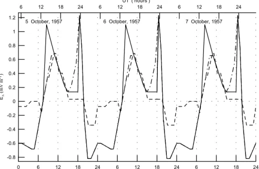
Fig. 1. Diurnal variations of E3on 7 October 1957. The empirical F-region quiet time vertical drift velocity over the geomagnetic equator
presented in Fig. 8 of Scherliess and Fejer (1999) for high solar activity and equinox conditions was used to find the equatorial value of
E3(dash-dotted line). Solid line shows the empirical equatorial electric field which was modified in the time range between 07:27 LT and
11:00 LT and between 15:00 LT and 18:30 LT by the use of the comparison between the measured and modelled values of NmF2 and hmF2 at 00:00 UT and 16:00 UT. The average quiet time value of E3at the F-region altitudes over Arecibo (dashed line) is found from the average
quiet time perpendicular/northward F-region plasma drifts for equinox conditions presented in Fig. 2 of Fejer (1993).
There is evidence that the vertical E × B drift velocity varies with altitude at the geomagnetic equator (Pingree and Fejer, 1987). In the present study, the simplistic approach is used to calculate the dependence of E3on tge, where tgeis the local time at the geomagnetic equator for the magnetic longitude of each ionosonde station.
In the model, the value of E3(tge)over the geomagnetic equator given by the dash-dotted line in Fig. 1 is obtained from the empirical F-region quiet time equatorial vertical drift velocity presented in Fig. 8 of Scherliess and Fejer (1999) for high solar activity and equinox conditions. As it will be discussed later in Sect. 4, this empirical equatorial electric field is modified in the time range between 07:27 LT and 11:00 LT and between 15:0 LT and 18:30 LT by the use of the comparison between the measured and modelled night-time values of hmF2. The resulting equatorial magnitude of
E3(tge), which is used in the model calculations is shown by the solid line in Fig. 1. The average quiet time value of E3 at the F-region altitudes over Arecibo (dashed line in Fig. 1) is found from Fig. 2 of Fejer (1993), where the average quiet time perpendicular/northward F-region plasma drifts for high solar activity and equinox conditions is presented.
Equations (A11), (A12), and (A15) determine the trajec-tory of the ionospheric plasma perpendicular to magnetic field lines and the moving coordinate system. It follows from Eq. (A11) that time variations of U caused by the ex-istence of the E3 component of the electric field are deter-mined by time variations of the 3 component, E3eff, of the effective electric field given by Eq. (A12). We have to
take into account that the magnetic field lines are “frozen” in the ionospheric plasma (see Sect. A2.5.1 of Appendix A). As a result, E3eff(t )is not changed along magnetic field lines (see Eq. A15). The equatorial and Arecibo values of
E3(tge)are used to find the equatorial and Arecibo values of E3eff(tge)from Eqs. (A12) and (A15). The equatorial value of E3eff(tge)(the equatorial E3(tge)is given by the solid line in Fig. 1) is used for magnetic field lines with an apex altitude, hap = Req −RE, less than 600 km, where
Reqis the equatorial radial distance of the magnetic field line from the Earth’s center and RE is the Earth’s radius. The Arecibo value of E3eff(tge)(the Arecibo E3(tge)is given by the dashed line in Fig. 1) is used if the apex altitude is greater than 2 126 km. Linear interpolation of the equatorial and Arecibo values of E3eff(tge)is employed at the inter-mediate apex altitudes.
The model starts at 15:12 UT on 5 October 1957. This UT corresponds to 10:00 LT at the geomagnetic equator and 351.9◦of the geomagnetic longitude (see explanations of the value of the geomagnetic longitude in Sect. 3). First of all, the steady-state Ni, Ne, Ti, and Teare found by the use of the model of the ionosphere and plasmasphere with E3=0 (i.e. without the E × B drift velocity). It means that the one-dimensional time dependent Eqs. (A1), (A6), and (A7) of Appendix A are solved along each computational grid dipole magnetic field line at 10:00 UT on 5 October 1957, to ob-tain the Ni, Ne, Ti, and Te initial conditions. These steady-state daytime values of Ni, Ne, Ti, and Te are used as ini-tial conditions to solve the two-dimensional, time dependent
A. V. Pavlov: New method in computer simulations of electron and ion densities and temperatures 1605 350 400 450 500 550 hm F 2 ( k m ) -30 -20 -10 0 10 20 30
Geomagnetic latitude (degrees)
20 30 40 Nm F 2 ( 1 0 5 cm -3 ) 400 500 600 700 hm F 2 ( k m ) 0 10 20 30 40 50 Nm F 2 ( 1 0 5 cm -3 ) 00:00 UT, empirical EΛ 16:00 UT, empirical EΛ 00:00 UT, empirical EΛ 16:00 UT, empirical EΛ -30 -20 -10 0 10 20 30
Geomagnetic latitude (degrees)
Fig. 2 00:00 UT, modified EΛ 00:00 UT, modified EΛ 16:00 UT, modified EΛ 16:00 UT, modified EΛ a b c d e f g h
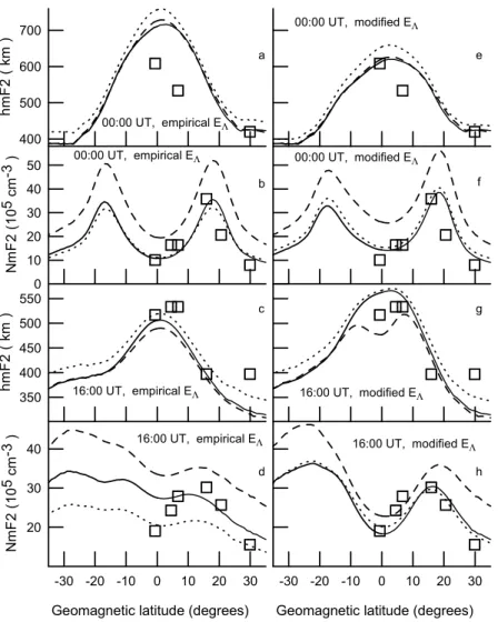
Fig. 2. Observed (squares) and calculated (lines) hmF2 and NmF2 at 00:00 UT (Panels a, b, e, f) and 16:00 UT (Panels c, d, g, h) on 7
October 1957. Left panels (a), (b), (c), (d) show the model results when the original equatorial perpendicular plasma drift of Scherliess and Fejer (1999) given by the dash-dotted line in Fig. 1 is used. Right panels (e), (f), (g), (h) show the model results when the empirical equatorial electric field found the equatorial perpendicular plasma drift velocity of Scherliess and Fejer (1999) was modified in the time range between 07:27 LT and 11:00 LT and between 15:00 LT and 18:30 LT (this modified equatorial electric field is shown by a solid line in Fig. 1). Dashed lines show the model results when the original NRLMSISE-00 neutral temperature and densities are used. Solid lines show the model results when the NRLMSISE-00 model [O] was decreased by a factor of 1.7 from 16:12 UT to 23:12 UT (from 11:00 LT to 18:00 LT, where LT is the local time at the geomagnetic equator and 351.9◦of the geomagnetic longitude) during all model simulation period. Dotted lines show the model results when the NRLMSISE-00 model [N2] and [O2] were increased by a factor of 2.1 from 16:12 UT to 23:12 UT during all
model simulation period. The vibrationally excited N2(v > 0) and O2(v > 0) are included in the model and the EUVAC solar flux model
is used as the input model parameter in all model calculations presented in Fig. 2. The difference between UT and the local time at the geomagnetic equator is 05:12.
Eqs. (A1), (A6), and (A7) of Appendix A with the model value of E3. The model is run from 15:12 UT on 5 October 1957 to 24:00 UT on 6 October 1957 before model results are used.
3 Solar geophysical conditions and data
The value of the geomagnetic Kpindex was between 0 and 2 for the studied time period of 7 October 1957. It should be noted that when the thermosphere is disturbed, it takes time for it to relax back to its initial state, and this thermosphere
relaxation time determines the time for the disturbed iono-sphere to relax back to the quiet state. It means that not every time period with Kp≤3 can be considered as a magnetically quiet time period. The characteristic time of the neutral com-position recovery after a storm impulse event ranges from 7 to 12 hours, on average (Hedin, 1987), while it may need up to days for all altitudes down to 120 km in the atmosphere to recover completely back to the undisturbed state of the at-mosphere (Richmond and Lu, 2000). The value of Kp was between 0 and 3 for the previous 4–6 October 1957 time pe-riod, i.e. the studied time period of 7 October 1957 can be
1606 A. V. Pavlov: New method in computer simulations of electron and ion densities and temperatures considered as a magnetically quiet time period. The F10.7
solar activity index was 254 on 7 October 1957, while the 81-day averaged F10.7 solar activity index was 234.
Our study is based on hourly critical frequencies fof2, and foE, of the F2 and E-layers, and the maximum usable frequency parameter, M(3000)F2, data from the Huancayo, Chiclayo, Talara, Bogota, Panama, and, Puerto Rico iono-spheric sounder stations available on the Ionoiono-spheric Digi-tal Database of the National Geophysical Data Center, Boul-der, Colorado. Locations of these ionospheric sounder sta-tions are shown in Table 1. The first five sounders at low latitude are within ±3.5◦ geomagnetic longitude of one an-other. As a result, all model simulations are carried out for the geomagnetic longitude of 351.9◦. To complete the pic-ture of the latitude dependence of NmF2 and hmF2 varia-tions, we compare the modeled NmF2 and hmF2 at the geo-magnetic longitude of 351.9◦with Nmf2 and hmF2 measured by the Puerto Rico ionosonde station with geomagnetic lon-gitude 2.8◦. The Puerto Rico sounder departs slightly from the near conjugacy of the Huancayo, Chiclayo, Talara, Bo-gota, and Panama ionospheric sounder stations, but this geo-magnetic longitude deviation is nonsignificant for our study because the equatorial anomaly effects are less pronounced at the Puerto Rico sounder in comparison with those at the first five sounders. The values of the peak density, NmF2, of the F2-layer is related to the critical frequencies fof2 as
NmF2 = 1.24 · 1010fof22, where the unit of NmF2 is m−3, the unit of fof2 is MHz. To determine the ionosonde val-ues of hmF2, we use the relation between hmF2 and the values of M(3000)F2, fof2, and foE recommended by Du-deney (1983) from the comparison of different approaches as hmF2 = 1490/[M(3000)F2 + 1M]-176, where 1M = 0.253/(fof2/foE−1.215)−0.012. If there are no foE data, then it is suggested that 1M = 0, i.e. the hmF2 formula of Shi-mazaki (1955) is used.
4 Results
4.1 Equatorial perpendicular electric field modification In Fig. 2, geomagnetic latitude plots are shown of hmF2 and
NmF2 at 00:00 UT (panels (a), (b), (e), and (f)) and 16:00 UT
(panels (c), (d), (g), and (h)) on 7 October 1957 from the ionospheric sounder station measurements (squares) and model calculations (solid, dotted, and dashed lines). Four left panels (a), (b), (c), and (d) show the model results when the original equatorial perpendicular plasma drift of Scherliess and Fejer (1999), given by the dash-dotted line in Fig. 1, is used. Four right panels (e), (f), (g), and (h) show the model results when the empirical equatorial electric field, found from the equatorial perpendicular plasma drift veloc-ity of Scherliess and Fejer (1999), was modified in the time range between 07:27 LT and 11:00 LT and between 15:00 LT and 18:30 LT (this modified equatorial electric field is shown by a solid line in Fig. 1). Dashed lines show the model results when the original NRLMSISE-00 neutral temperature and
densities are used. Solid lines show the model results when the NRLMSISE-00 model [O] was decreased by a factor of 1.7 from 16:12 UT to 23:12 UT (from 11:00 LT to 18:00 LT, where LT is the local time at the geomagnetic equator and 351.9◦of the geomagnetic longitude) during all model sim-ulation periods. Dotted lines show the model results when the NRLMSISE-00 model [N2] and [O2] were increased by a factor of 2.1 from 16:12 UT to 23:12 UT during all model simulation periods. The vibrationally excited N2(v > 0) and O2(v > 0) are included in the model, and the EUVAC solar flux model is used as the input model parameter in all model calculations presented in Fig. 2.
The comparison between the results shown in the two up-per panels (a) and (e) of Fig. 2 clearly indicates that there is a large disagreement between the measured and modelled
hmF2 at 00:00 UT on 7 October 1957, if the equatorial
up-ward E × B drift given by Scherliess and Fejer (1999) is used. The results presented in panels (a) and (b) of Fig. 2 pro-vide epro-vidence that we can match the measured and modeled
NmF2 using the corrected neutral densities. However, the
corrections of the NRLMSISE-00 model [O], [N2], or [O2] do not bring the measured and modeled hmF2 into agree-ment. We conclude that this disagreement in hmF2 is caused by the long time duration of the pre-reversal strengthening of the equatorial upward E × B drift given by Scherliess and Fejer (1999). The high estimate of this pulse duration in E3 leads to unreal, high-modeled F2 peak altitudes at 00:00 UT. Our calculations presented in the panels (e) and (f) of Fig. 2 provide evidence that, to bring the measured and modeled F2-region main peak altitudes into agreement, the magnitude of E3 has to be approximately constant in the time range between 15:00 LT and 18:00 LT with the following peak in
E3, which has a shorter time width in comparison with the time duration of the pre-reversal strengthening of the orig-inal equatorial perpendicular plasma drift given by Scher-liess and Fejer (1999). Fejer et al. (1989) show solar max-imum ion vertical drifts over Jicamarca, which is very close to Huancayo, near the magnetic equator. The pre-reversal enhancements during quiet equinox periods can begin as late as 18:00 LT and peak after 19:00 LT, although the average enhancements are earlier and broader. In addition, Batista et al. (1986) estimate the pre-reversal enhancement at Huan-cayo to peak between 18:00 LT and 19:00 LT based on hmF2 changes during equinox solar maximum conditions. Thus, our delay of the pre-reversal enhancement until 18:00 LT is in agreement with the observed day-to-day variability at Ji-camarca, and previous estimates for Huancayo.
The principal feature of the equatorial anomaly is that the crest-to-trough ratio is increased with increasing up-ward E × B drift (Dunford, 1967; Su et al., 1997; Rish-beth, 2000). The measurements show that, by mid-afternoon (15:00 UT), the equatorial anomaly crests are forming away from the geomagnetic equator, while the model calculations with the equatorial E3(tge), given by the dash-dotted line in Fig. 1, produce the onset of the equatorial anomaly crest for-mation close to 16:00 UT (see lines in panels (c) and (d) of Fig. 2). The disagreement between the sizes of the
equato-A. V. Pavlov: New method in computer simulations of electron and ion densities and temperatures 1607
Table 1. Ionosonde station names and locations
Ionosonde Geographic Geographic Geomagnetic Geomagnetic station latitude longitude latitude longitude Huancayo -12.0 284.6 -0.65 354.5 Chiclayo -6.7 280.1 4.5 349.9 Talara -4.5 278.6 6.7 348.4 Bogota 4.5 285.8 15.9 355.4 Panama 9.4 280.1 20.6 349.3 Puerto Rico 18.5 292.8 29.9 2.8
rial trough in the measured (squares in panel (d) of Fig. 2) and modeled (lines in panel (d) of Fig. 2) NmF2 at 16:00 UT can be explained by disagreements between the chosen and unknown real values of E3(tge)on 7 October 1957. The re-sults presented in panel (d) of Fig. 2 provide evidence that we cannot match the measured and modeled NmF2 and the sizes of the measured and modeled equatorial troughs using the corrections of the NRLMSISE-00 model [O], [N2], or [O2].
Our calculations show that a strengthening of the equato-rial upward E × B drift before 17:00 UT on 7 October 1957 leads to an increase in the northern and southern depths of the equatorial NmF2 trough (these depths can be expressed as ratios of NmF2 at F2-region northern and southern crests to an equatorial NmF2) at 17:00 UT on 7 October 1957. The modification of E3(tge) is shown by a solid line in Fig. 1. This modification, which was carried out in the time range between 07:27 LT and 11:00 LT, includes the strengthen-ing of E3 and the time shift of the peak in E3(tge) rela-tive to the peak in E3(tge), shown by the dash-dotted line in Fig. 1. The first maximum (E3=1.1 mVm−1) of the mod-ified E3(tge) occurs at 08:30 LT while the first maximum (E3 =0.66 mVm−1) of E3(tge), given by the dash-dotted line in Fig. 1, is located between 10:00 LT and 11:00 LT. It should be noted that the revised magnitude of the first peak in E3is close to the magnitude of the second peak in
E3, although the second peak is expected to be about dou-ble the size of the first peak in solar maximum (Fesen et al., 2000). However, the Fejer et al. (1995) quiet-time equinox model from the AE-E satellite observations during moder-ate to high solar flux conditions at 260◦E suggest a morn-ing peak at 09:30 LT, which is nearly equal to the sharper evening reversal peak, similar to our proposed changes. The comparison between the squares and solid line in panel (h) of Fig. 2 shows that the northern depth of the equatorial NmF2 trough in the calculated NmF2 is approximately consistent with the measured depth, if the modified E3(tge) is used. The model NmF2 is higher than the observations with the anomaly crest shifted poleward, if the original NRLMSISE-00 model is used (see dashed line in panel (h) of Fig. 2). Panel (g) of Fig. 2 shows that the agreement between mea-sured and modeled hmF2 is somewhat worse. It should be noted that the model with the modified value of E3(tge) pro-duces the onset of the equatorial anomaly crest formation
close to 15:00 UT, in agreement with the measured onset of the equatorial anomaly crest formation given by ionosonde stations.
As a result, the equatorial electric field, shown by the solid line in Fig. 1, and the Arecibo value of E3(tge), shown by the dashed line in Fig. 1, are used in all subsequent model calculations presented in this paper, as described in Sect. 2. 4.2 Evaluation of uncertainties in model calculations of
NmF2 and hmF2 from the comparison between neutral
atmosphere models and between the solar flux models as input model parameters
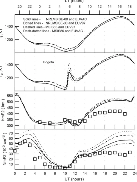
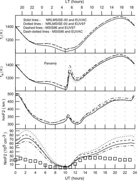
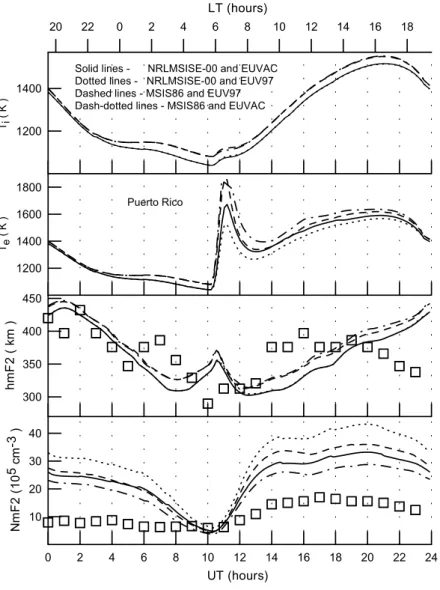
The measured (squares) and calculated (lines) NmF2 and
hmF2 are displayed in the two lower panels of Figs. 3–8 for
the 7 October 1957 time period above the Huancayo (Fig. 3), Chiclayo (Fig. 4), Talara (Fig. 5), Bogota (Fig. 6), Panama (Fig. 7), and Puerto Rico (Fig. 8) ionosonde stations. The re-sults obtained from the model of the ionosphere and plasma-sphere, using the combinations of the original NRLMSISE-00 or MSIS-86 neutral temperature and density models and the EUVAC or EUV97 solar flux models as the input model parameters, are shown by solid lines (the NRLMSISE-00 model in combination with the EUVAC model), dotted lines (the NRLMSISE-00 model in combination with the EUV97 model), dash-dotted lines (the MSIS-86 model in combina-tion with the EUVAC model), and dashed lines (the MSIS-86 model in combination with the EUV97 model).
The differences in original neutral densities and temper-atures from the NRLMSISE-00 and MSIS-86 models result in the differences between solid and dash-dotted lines (the EUVAC solar flux model is used) and between dotted and dashed lines (the EUV97 solar flux model is used). We found that the use of the NRLMSISE-00 model, as opposed to the MSIS-86 model, leads to the highest possible increase in the calculated NmF2 by a maximum factor of 1.29, 1.23, 1.22, 1.28, 1.30, and 1.39 and to the highest possible decrease in the calculated hmF2 by 38, 42, 40, 22, 22 and 23 km above the Huancayo, Chiclayo, Talara, Bogota, Panama, and Puerto Rico ionosonde stations, respectively. The use of the EUV97 solar flux model as opposed to the EUVAC solar flux model leads to the increase in the calculated NmF2 by a factor of 1.13–1.34 and to the highest possible variations in calculated
1608 A. V. Pavlov: New method in computer simulations of electron and ion densities and temperatures 2 300 350 400 450 500 550 600 650 700 hm F 2 ( k m ) 0 2 4 6 8 10 12 14 16 18 20 22 24 UT (hours) Fig. 3 10 20 30 40 Nm F 2 ( 1 0 5 cm -3 ) 1200 1400 Ti ( K ) 1200 1400 Te ( K )
Solid lines - NRLMSISE-00 and EUVAC Dotted lines - NRLMSISE-00 and EUV97 Dashed lines - MSIS86 and EUV97 Dash-dotted lines - MSIS86 and EUVAC
Huancayo
20 22 0 2 4 6 8 10 12 14 16 18
LT (hours)
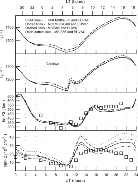
Fig. 3. Observed (squares) and cal-culated (lines) NmF2 and hmF2 (two lower panels), and electron and O+ion temperatures (two upper panels) at the F2-region main peak altitude above the Huancayo ionosonde station on 7 Oc-tober 1957. The results obtained from the model of the ionosphere and plas-masphere using the combinations of the original NRLMSISE-00 or original MSIS-86 neutral temperature and den-sities model and the EUVAC or EUV97 solar flux models as the input model pa-rameters are shown by solid lines (the NRLMSISE-00 model in combination with the EUVAC model), dotted lines (the NRLMSISE-00 model in combi-nation with the EUV97 model), dash-dotted lines (the MSIS-86 model in combination with the EUVAC model), dashed lines (the MSIS-86 model in combination with the EUV97 model). LT is the local time at the Huancayo ionosonde station.
Our calculations clearly show that the best agreement be-tween the measured and modeled electron densities is ob-tained if the MSIS-86 neutral densities and temperature in combination with the EUVAC solar flux (dash-dotted lines in Figs. 3–8) are used as the input model parameters. At the same time, the NRLMSISE-00 model is the outgrowth of the MSIS-86 model, and we have a right to expect that the NRLMSISE-00 model describes real neutral temperature and densities variations more accurately in comparison to the MSIS-86 model. Therefore, the NRLMSISE-00 neutral tem-perature and density model of Picone et al. (2000, 2002), and the EUVAC solar flux model of Richards et al. (1994) are used in the further model calculations presented in this work. 4.3 Electron and ion temperature variations
Two upper panels of Figs. 3–8 show the electron, Te, and ion,
Ti, temperatures at the F2-region main peak altitude calcu-lated for the 7 October 1957 time period above the Huancayo (Fig. 3), Chiclayo (Fig. 4), Talara (Fig. 5), Bogota (Fig. 6), Panama (Fig. 7), and Puerto Rico (Fig. 8) ionosonde stations.
The results obtained from the model of the ionosphere and plasmasphere, using the combinations of the NRLMSISE-00 or MSIS-86 neutral temperature and density models and the EUVAC or EUV97 solar flux models as the input model parameters, are shown by solid lines (the NRLMSISE-00 model in combination with the EUVAC model), dotted lines (the NRLMSISE-00 model in combination with the EUV97 model), dash-dotted lines (the MSIS-86 model in combina-tion with the EUVAC model), and dashed lines (the MSIS-86 model in combination with the EUV97 model). It is evident from Figs. 3–8 that the electron and ion temperature changes created by the difference between the NRLMSISE-00 and MSIS-86 neutral temperatures and number densities or by the difference between the EUV97 and EUVAC solar fluxes are negligible.
The electron and ion temperatures start to increase from their night-time values close to 10:12 UT. The electron tem-perature reaches a morning peak at about 10:52–11:12 UT, above the ionosonde stations of Table 1, while the ion tem-peratures above all the ionosonde stations presented in Ta-ble 1 have no morning peaks at hmF2. Following the
morn-A. V. Pavlov: New method in computer simulations of electron and ion densities and temperatures 1609 3 300 350 400 450 500 550 600 650 hm F 2 ( k m ) 0 2 4 6 8 10 12 14 16 18 20 22 24 UT (hours) Fig. 4 10 20 30 40 Nm F 2 ( 1 0 5 cm -3 ) 1200 1400 Ti ( K ) 1200 1400 Te ( K )
Solid lines - NRLMSISE-00 and EUVAC Dotted lines - NRLMSISE-00 and EUV97 Dashed lines - MSIS86 and EUV97 Dash-dotted lines - MSIS86 and EUVAC
Chiclayo
20 22 0 2 4 6 8 10 12 14 16 18
LT (hours)
Fig. 4. From bottom to top, ob-served (squares) and calculated (lines) of NmF2, hmF2, electron temperatures and O+ ion temperatures at the F2-region main peak altitude above the Chiclayo ionosonde station on 7 Octo-ber 1957. LT is the local time at the Chiclayo ionosonde station. The curves are the same as in Fig. 3.
ing peak, there is a rapid decrease in the electron temperature, which reaches a minimum at around 11:32–13:12 UT. After the electron temperature minimum, the electron temperature increases again above the ionosonde stations.
The peak values in the electron and ion temperatures above all the ionosonde stations presented in Table 1 occur at about 20:32–21:22 UT. Our calculations show that the magnitudes of the electron and ion temperatures at hmF2 are close to the neutral temperature at hmF2 during most of the daytime con-ditions. As a result, the peak values in the electron and ion temperatures result from the peak in the neutral temperature at hmF2, which occurs very close to the time of the peaks in the electron and ion temperatures above the ionosonde sta-tions presented in Table 1.
It is well known that in the ionospheric F-region, there is an inverse relationship between electron temperature and electron density, i.e. greater electron densities produce lower electron temperatures. As a result, the electron temperature is close to the neutral temperature during most of the day-time period at hmF2 altitudes at solar maximum, due to high magnitudes of electron cooling rates in comparison with the
input of the electron heat flow along the magnetic field line in the daytime electron temperature variations.
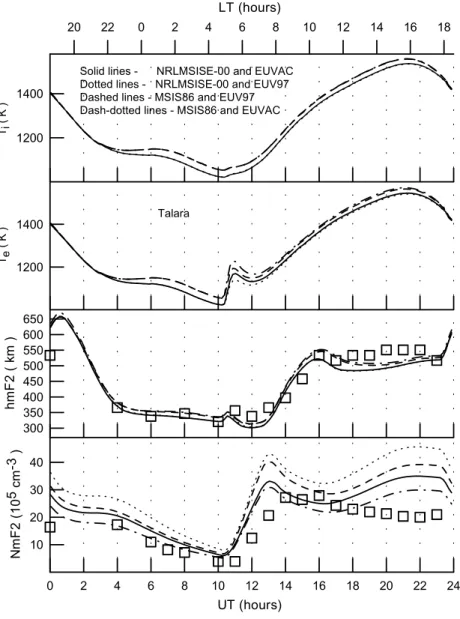
Electron and ion temperatures profiles measured at Jica-marca close to the geomagnetic equator between June 1965 and November 1966 are such that Te > Ti between about 200 km and 300 km during daytime conditions, Te ≈Ti ≈ const between about 300 km and 500 km, and the value of Te is close to the neutral temperature in this daytime isothermal altitude region (McClure, 1969; Schunk and Nagy, 1978). This daytime electron and ion isothermal region can come up to 600 km (Bailey et al., 1975). Throughout this region the electron thermal conduction term in the thermal balance equation of electrons is negligible in comparison with cool-ing of electrons due to collisions of thermal electrons with ions and neutral gases (Bailey et al., 1975; Schunk and Nagy, 1978). Our calculations show that the values of the electron temperatures at F2-region altitudes become almost indepen-dent of the electron heat flow along the magnetic field line above the Huancayo (Fig. 3), Chiclayo (Fig. 4), and Talara (Fig. 5) ionosonde stations because the near-horizontal mag-netic field inhibits this heat flow of electrons. The increase
1610 A. V. Pavlov: New method in computer simulations of electron and ion densities and temperatures 4 300 350 400 450 500 550 600 650 hm F 2 ( k m ) 0 2 4 6 8 10 12 14 16 18 20 22 24 UT (hours) Fig. 5 10 20 30 40 Nm F 2 ( 1 0 5 cm -3 ) 1200 1400 Ti ( K ) 1200 1400 Te ( K )
Solid lines - NRLMSISE-00 and EUVAC Dotted lines - NRLMSISE-00 and EUV97 Dashed lines - MSIS86 and EUV97 Dash-dotted lines - MSIS86 and EUVAC
Talara
20 22 0 2 4 6 8 10 12 14 16 18
LT (hours)
Fig. 5. From bottom to top, ob-served (squares) and calculated (lines) of NmF2, hmF2, electron temperatures and O+ ion temperatures at the F2-region main peak altitude above the Talara ionosonde station on 7 October 1957. LT is the local time at the Talara ionosonde station. The curves are the same as in Fig. 3.
in geomagnetic latitude leads to the increase in the effects of the electron heat flow along the magnetic field line on Te.
It follows from the electron and ion temperatures profiles measured at Jicamarca that the enlargement of the altitude region with Te > Ti occurs at sunrise at all heights to at least 600 km (McClure, 1969). Our calculations show that at sunrise, there is a rapid heating of the ambient electrons by photoelectrons, and the difference between the electron and neutral temperatures could be increased because night-time electron densities are less than those by day, and the electron cooling during morning conditions is less than that by day. This expands the altitude region at which Te > Ti near the equator, and leads to the sunrise electron tempera-ture peaks at hmF2 altitudes above the ionosonde stations. After the abrupt increase at sunrise, the electron temperature decreases, owing to the increasing electron density due to the increase in the cooling rate of thermal electrons and due to the decrease in the relative role of the electron heat flow along the magnetic field line in comparison with cooling of
thermal electrons. As a result, the morning electron temper-ature peaks which are found above the ionosonde stations at
hmF2 altitudes are explained by these physical processes.
Early studies have pointed out that the radar Temeasured at Jicamarca are lower than Temeasured by using probes on satellites, and there was a problem with unreal night-time radar Te < Ti (McClure et al., 1973; Aponte et al., 2001). This problem was solved by Sulzer and Gonzalez (1999) and Aponte et al. (2001), who found that electron-electron and electron-ion Coulomb collisions are responsible for the ad-ditional incoherent backscatter spectral narrowing above Ji-camarca, leading to the change in the measured Te/Ti ratio. Specifically, Te =Ti at night, at F-region altitudes above Ji-camarca (Aponte et al., 2001). In agreement with this conclu-sion, our calculations show that Te=Ti at night, at F-region altitudes close to the geomagnetic equator.
The relative magnitudes of the cooling rates are of par-ticular interest for understanding the main processes which determine the electron temperature. The model of the
iono-A. V. Pavlov: New method in computer simulations of electron and ion densities and temperatures 1611 5 300 350 400 450 500 550 hm F 2 ( k m ) 0 2 4 6 8 10 12 14 16 18 20 22 24 UT (hours) Fig. 6 10 20 30 40 50 60 70 Nm F 2 ( 1 0 5 cm -3 ) 1200 1400 Ti ( K ) 1200 1400 Te ( K )
Solid lines - NRLMSISE-00 and EUVAC Dotted lines - NRLMSISE-00 and EUV97 Dashed lines - MSIS86 and EUV97 Dash-dotted lines - MSIS86 and EUVAC
Bogota
20 22 0 2 4 6 8 10 12 14 16 18
LT (hours)
Fig. 6. From bottom to top, ob-served (squares) and calculated (lines) of NmF2, hmF2, electron temperatures and O+ ion temperatures at the F2-region main peak altitude above the Bo-gota ionosonde station on 7 October 1957. LT is the local time at the Bo-gota ionosonde station. The curves are the same as in Fig. 3.
sphere and plasmasphere uses the electron cooling rates due to electron-ion Coulomb collisions and elastic collisions of electrons with N2, O2, O, He and H, the thermal electron impact excitation of O2(a11g), O2(b1Pg+), and the fine structure levels of the ground state of atomic oxygen, the rates of electron cooling through vibrational and rotational excitation of N2 and O2, and the electron energy loss aris-ing from electron-impact-induced transitions 3P → 1D for atomic oxygen (see Sect. A2.2 of Appendix A). The rela-tive role of the electron cooling rates was evaluated. We found that the main cooling rates of thermal electrons on 7 October 1957, are electron-ion Coulomb collisions, vibra-tional excitation of N2 and O2, and rotational excitation of N2. The relative role of the cooling rates of thermal elec-trons by low-lying electronic excitation of O2(a11g) and O2(b1Pg+), from rotational excitation of O2, in collision of O(3P) with thermal electrons with the O(1D) formation, and by the atomic oxygen fine structure excitation, is negligible in comparison with the effects of the main cooling rates on
the electron temperature for the geomagnetically quiet period on 7 October 1957.
4.4 Effects of corrections in the NRLMSISE-00 model [O] or [N2] and [O2] on the ionosphere.
Figures 3–8 show that the calculated NmF2 is systematically higher than the measured one during most of the studied time period. We can expect that the neutral models have some in-adequacies in predicting the number densities with accuracy, and we have to change the number densities by correction factors at all altitudes, to bring the modeled electron densi-ties into agreement with the measurements.
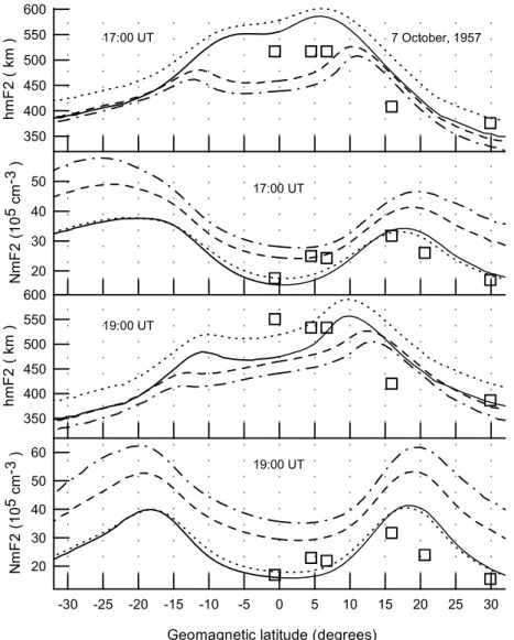
The comparison between the measured (squares) and mod-eled (lines) NmF2 and hmF2 latitude variations are shown in Fig. 9, at 17:00 UT (two upper panels) and 19:00 UT (two lower panels) on 7 October 1957 and in Fig. 10 at 21:00 UT (two upper panels) and 23:00 UT (two lower panels) on 7 October 1957. Dashed lines show the model results when the original NRLMSISE-00 neutral temperature and
densi-1612 A. V. Pavlov: New method in computer simulations of electron and ion densities and temperatures 6 300 350 400 450 500 hm F 2 ( k m ) 0 2 4 6 8 10 12 14 16 18 20 22 24 UT (hours) Fig. 7 10 20 30 40 50 60 70 80 90 Nm F 2 ( 1 0 5 cm -3 ) 1200 1400 Ti ( K ) 1200 1400 Te ( K )
Solid lines - NRLMSISE-00 and EUVAC Dotted lines - NRLMSISE-00 and EUV97 Dashed lines - MSIS86 and EUV97 Dash-dotted lines - MSIS86 and EUVAC
Panama
20 22 0 2 4 6 8 10 12 14 16 18
LT (hours)
Fig. 7. From bottom to top, ob-served (squares) and calculated (lines) of NmF2, hmF2, electron temperatures and O+ ion temperatures at the F2-region main peak altitude above the Panama ionosonde station on 7 October 1957. LT is the local time at the Panama ionosonde station. The curves are the same as in Fig. 3.
ties are used. Solid lines show the model results when the NRLMSISE-00 model [O] was decreased by a factor of 1.7 by day, from 16:12 UT to 23:12 UT (from 11:00 LT to 18:00 LT) at all altitudes without NRLMSISE-00 [N2] and [O2] corrections, where LT is the local time at the geomag-netic equator and 351.9◦of the geomagnetic longitude) dur-ing the model simulation period. Dash-dotted and dotted lines will be explained later. One can see from Figs. 9 and 10 that the NRLMSISE-00 model with the decreased [O] im-proves the agreement with the measured NmF2 and hmF2.
We can also expect that the NRLMSISE-00 model has some inadequacies in predicting the actual N2and O2 num-ber densities with accuracy. The values of the NRLMSISE-00 [N2] and [O2] were increased by a factor of 2.1 from 16:12 UT to 23:12 UT at all altitudes without NRLMSISE-00 [O] corrections to compare the effects of the NRLMSISE-00 [N2] and [O2] correction on NmF2 and hmF2 with those ob-tained from the NRLMSISE-00 [O] correction. The resulting model NmF2 and hmF2 are shown by dotted lines in Figs. 9 and 10. In general, the use of the increased NRLMSISE-00 N2and O2model densities brings the modeled and measured
NmF2 and hmF2 into satisfactory agreement.
The comparison between the NRLMSISE-00 [N2] and [O2] increases and the NRLMSISE-00 [O] decrease does not show similarity and consistency in their effects on
hmF2. Above the ionosonde stations presented in Table 1,
the NRLMSISE-00 [O] decrease leads to the calculated
hmF2, which are less than that given by the model with the
NRLMSISE-00 [N2] and [O2] correction, and this difference does not exceed the value of 48 km. However, this differ-ence in the calculated hmF2 is not large enough to determine which of these two kinds of corrections of the NRLMSISE-00 model are preferred by comparing the measured and mod-elled hmF2.
The comparison between the NRLMSISE-00 [N2] and [O2] increases and the NRLMSISE-00 [O] decrease do show similarity and consistency in their effects on NmF2. Our cal-culations cannot provide evidence in favor of reducing [O] in comparison with increasing [N2] and [O2]. The reactions be-tween O+(4S) ions and vibrationally unexcited and excited N2provide the main input in the loss rate of O+(4S) ions at F-region altitudes, in comparison with that given by the
reac-A. V. Pavlov: New method in computer simulations of electron and ion densities and temperatures 1613 7 300 350 400 450 hm F 2 ( k m ) 0 2 4 6 8 10 12 14 16 18 20 22 24 UT (hours) Fig. 8 10 20 30 40 Nm F 2 ( 1 0 5 cm -3 ) 1200 1400 Ti ( K ) 1200 1400 1600 1800 Te ( K )
Solid lines - NRLMSISE-00 and EUVAC Dotted lines - NRLMSISE-00 and EUV97 Dashed lines - MSIS86 and EUV97 Dash-dotted lines - MSIS86 and EUVAC
Puerto Rico
20 22 0 2 4 6 8 10 12 14 16 18
LT (hours)
Fig. 8. From bottom to top, ob-served (squares) and calculated (lines) of NmF2, hmF2, electron temperatures and O+ ion temperatures at the F2-region main peak altitude above the Puerto Rico ionosonde station on 7 Oc-tober 1957. LT is the local time at the Puerto Rico ionosonde station. The curves are the same as in Fig. 3.
tions between O+(4S) ions and vibrationally unexcited and excited O2. It follows from the calculations that the [O]/[N2] ratio determines the value of NmF2. Therefore, we can only conclude from our results that it is necessary to decrease the NRLMSISE-00 model [O]/[N2] ratio by a factor of 1.7–2.1, to bring the modeled and measured hmF2 and NmF2 on 7 October 1957 into agreement.
4.5 Effects of vibrationally excited oxygen and nitrogen on
NmF2 and hmF2
Dash-dotted lines in Figs. 9 and 10 display the calculated
NmF2 and hmF2 on 7 October 1957, when vibrationally
ex-cited N2(v > 0) and O2(v > 0) are not included in the model calculations of the loss rate of O+(4S) ions, and the original NRLMSISE-00 neutral temperature and density model and the EUVAC solar flux model are used. The heating rate of electrons due to the de-excitation of vibrationally excited N2 and O2 is taken into account in all model calculations (for more details, see Pavlov, 1998a, c; Pavlov and Foster, 2001). As Figs. 9 and 10 show, there is a large increase in
the modeled NmF2 and a large decrease in the modeled
hmF2 without the vibrational excited nitrogen and oxygen
molecules. Both the measured NmF2 and hmF2 are not re-produced by the model without N2(v > 0) and O2(v > 0) in the loss rate of O+(4S) ions, and the inclusion of vibra-tionally excited N2 and O2 in the loss rate of O+(4S) ions brings the model and data into better agreement.
Dashed lines in Figs. 9 and 10 represent the results ob-tained from the model with the effects of vibrationally ex-cited N2(v > 0) and O2(v > 0) on the O+(4S) loss rate when the original NRLMSISE-00 neutral temperature and density model, and the EUVAC solar flux model are used. There-fore, the comparison between dashed and dash-dotted lines show the effects of vibrationally excited oxygen and nitrogen on NmF2 and hmF2. It follows from the model calculations that the increase in the loss rate of O+(4S) ions, due to the vibrational excited N2and O2, leads to the decrease in the calculated NmF2 by a factor of 1.06–1.44 and to the increase in the calculated hmF2, up to the maximum value of 32 km in the low-latitude ionosphere between -30◦and +30◦of the geomagnetic latitude.
1614 A. V. Pavlov: New method in computer simulations of electron and ion densities and temperatures 8 350 400 450 500 550 600 h m F 2 ( k m ) -30 -25 -20 -15 -10 -5 0 5 10 15 20 25 30
Geomagnetic latitude (degrees) Fig. 9 20 30 40 50 60 Nm F 2 ( 1 0 5 cm -3 ) 350 400 450 500 550 600 hm F 2 ( km ) 20 30 40 50 Nm F 2 ( 1 0 5 cm -3 ) 7 October, 1957 17:00 UT 19:00 UT 17:00 UT 19:00 UT
Fig. 9. Observed (squares) and calculated (lines) hmF2 and NmF2 at 17:00 UT (two upper panels) and 19:00 UT (two lower panels) on
7 October 1957. The measured hmF2 and NmF2 are taken from the ionospheric sounder station shown in Table 1. The results obtained from the model of the ionosphere and plasmasphere using the EUVAC solar flux model as the input model parameter. Dashed lines show the model results when the original NRLMSISE-00 neutral temperature and densities are used. Solid lines show the model results when the NRLMSISE-00 model [O] was decreased by a factor of 1.7 from 16:12 UT to 23:12 UT (from 11:00 LT to 18:00 LT, where LT is the local time at the geomagnetic equator and 351.9◦of the geomagnetic longitude) during all model simulation period. Dotted lines show the model results when the NRLMSISE-00 model [N2] and [O2] were increased by a factor of 2.1 from 16:12 UT to 23:12 UT during all model
simulation period. The vibrationally excited N2(v > 0) and O2(v > 0) are included in the model results shown by solid, dashed, and dotted
lines. Dash-dotted lines show the model results when N2(v > 0) and O2(v > 0) are not included in the calculations of the O+(4S) loss rate and the original NRLMSISE-00 model temperature and number densities were used. The difference between the universal time and the local time at the geomagnetic equator is 05:12.
It is found from numerical simulations of the mid-latitude ionosphere that the daytime magnitude of NmF2 should be reduced by about a factor of 2–3, due to enhanced vibrational excitation of N2 and O2 at high solar activity during geo-magnetically quiet and storm periods (see Pavlov and Foster, 2001 and references therein). It is apparent from the results of our calculations that the NmF2 decrease caused by the re-actions of O+(4S) ions with vibrationally excited N2and O2 is less at low geomagnetic latitudes, in comparison with that at middle geomagnetic latitudes at solar maximum.
The excitation of N2 and O2 by thermal electrons
pro-vides the main contribution to the values of N2 and O2 vi-brational excitations, if the electron temperature is higher than about 1600–1800 K at F-region altitudes (Pavlov, 1988, 1997, 1998b; Pavlov and Namgaladze, 1988; Pavlov and Buonsanto, 1997; Pavlov and Foster, 2001). The differ-ence between the vibrational temperature, TN2V , of N2and the neutral temperature, Tn , and the difference between the vibrational temperature, TO2V , of O2 and the neutral temperature increase with increasing electron temperature, and the noticeable differences TN2VTn > 50 − 200 K and
A. V. Pavlov: New method in computer simulations of electron and ion densities and temperatures 1615 9 350 400 450 500 550 hm F 2 ( k m ) -30 -25 -20 -15 -10 -5 0 5 10 15 20 25 30
Geomagnetic latitude (degrees) Fig. 10 10 20 30 40 50 60 70 Nm F 2 ( 1 0 5 cm -3 ) 350 400 450 500 550 hm F 2 ( k m ) 10 20 30 40 50 60 70 Nm F 2 ( 1 0 5 cm -3 ) 7 October, 1957 21:00 UT 23:00 UT 21:00 UT 23:00 UT
Fig. 10. Observed (squares) and calculated (lines) hmF2 and NmF2 at 21:00 UT (two upper panels) and 23:00 UT (two lower panels) on 7
October 1957. The difference between the universal time and the local time at the geomagnetic equator is 05:12. The curves are the same as in Fig. 9.
1800 K at F-region altitudes. Thus, as a result of low electron temperatures at F-region altitudes of the low latitude iono-sphere on 7 October 1957, the values of TN2V and TO2V are close to Tn, while the differences between Tn and the mid-dle latitude TN2V and TO2V are noticeable during daytime conditions at solar maximum (see Pavlov et al., 1999; Pavlov and Foster, 2001; Pavlov et al., 2001, and references therein). This is the first reason which explains the weaker decrease in the low-latitude NmF2 due to N2(v) and O2(v), in compari-son with that at middle geomagnetic latitudes.
The effects of N2(v) and O2(v) on middle-latitude NmF2 were usually evaluated by comparing the measured and mod-eled NmF2 using the original (Richards, 1991) or modi-fied (Pavlov and Buonsanto, 1997) Richards method, when model plasma drift velocities, caused by neutral winds, are found from the agreement between measured and modeled
hmF2. As a result, the middle-latitude model, including
vi-brationally excited N2 and O2 in the loss rate of O+(4S) ions produces hmF2 values very close to hmF2 produced by the middle-latitude model without including vibrationally excited N2 and O2. The low-latitude model described in Appendix A uses the HWW90 thermospheric wind model of Hedin et al. (1991) to calculate the thermospheric wind components and the corresponding plasma drift velocities along magnetic field lines. As Figs. 9 and 10 show, the low-latitude model, including N2(v) and O2(v) in the loss rate of O+(4S) ions produces hmF2 with values higher than hmF2 produced by the low-latitude model without including N2(v) and O2(v). As a result of including N2(v) and O2(v) in the loss rate of O+(4S) ions, the equatorial F2-layer is lifted to great heights, where the loss rate of O+(4S) ions is decreased, and this leads to an increase in NmF2, which is masked by the general decrease in NmF2 due to vibrationally excited N2 and O2. In other words, this additional increase in hmF2
de-1616 A. V. Pavlov: New method in computer simulations of electron and ion densities and temperatures creases the effects of vibrationally excited N2and O2on the
electron density in the low-latitude ionosphere.
5 Conclusions
A new theoretical model of the Earth’s low- and middle-latitude ionosphere and plasmasphere has been developed. The new model uses a new method in ionospheric and plas-maspheric simulations which is a combination of the Eule-rian and Lagrangian approaches in model simulations. The electron and ion continuity, and energy equations, are solved in a Lagrangian frame of reference which moves with an in-dividual parcel of plasma, with the local plasma drift velocity perpendicular to the magnetic and electric fields. As a re-sult, only the time-dependent, one-dimensional electron and ion continuity and energy equations are solved in this La-grangian frame of reference. The new method makes use of an Eulerian computational grid, which is fixed in space co-ordinates and chooses the set of the plasma parcels at every time step, so that all the plasma parcels arrive at points which are located between grid lines of the regularly spaced Eule-rian computational grid at the next time step. The solution values of electron and ion densities, and temperatures at the Eulerian computational grid, are obtained by interpolation.
Dipole orthogonal curvilinear coordinates q, U , and 3 are used, where q is aligned with, and U and 3 are perpendic-ular to, the magnetic field, and the U and 3 coordinates are constant along a dipole magnetic field line. Equations A11– A14, and Eqs. A15–A17, which determine the trajectory of the ionospheric plasma perpendicular to magnetic field lines and the moving coordinate system, are derived. It follows from these equations that time variations of U , caused by the existence of the E3component of the electric field, are deter-mined by time variations of the 3 component, E3eff, of the effective electric field and time variations of 3, caused by the existence of the EU component of the electric field, are de-termined by time variations of the U component, EUeff, of the effective electric field. It is shown that the magnetic field lines are “frozen” in the ionospheric plasma, if the values of E3eff and EUeff are not changed along magnetic field lines, and there is the interdependency given by Eq. A17 be-tween changes in EUeff in the 3 direction and changes in
E3eff in the U direction.
The Eulerian computational grid used consists of a distri-bution of the dipole magnetic field lines in the ionosphere and plasmasphere. One hundred dipole magnetic field lines are used in the model for each fixed value of the geomag-netic longitude. The number of the fixed nodes taken along each magnetic field line is 191. For each fixed value of the geomagnetic longitude, the region of study is a (q, U ) plane which is bounded by two dipole magnetic field lines. The low boundary dipole magnetic field line has the apex altitude of 150 km. The upper boundary dipole magnetic field line has the apex altitude of 4 491 km and intersects the Earth’s surface at two geomagnetic latitudes: ±40◦. The Eulerian
computational grid dipole magnetic field lines are distributed between these two boundary lines.
The model takes into account the offset between the ge-ographic and geomagnetic poles. The horizontal compo-nents of the neutral wind, which are used in calculations of the wind-induced plasma drift velocity along the magnetic field, are specified using the HWW90 wind model of Hedin et al. (1991). In the model, time-dependent ion continuity equations for the three major ions, O+(4S), H+ and He+ and for the minor ions, NO+, O2+, and N2+, are solved, and the approach of local chemical equilibrium is used to calculate steady-state number densities of O+(2D), O+(2P), O+(4P), and O+(2P∗) ions. The model includes the solution of time-dependent electron and ion energy balance equations. The model uses Boltzmann distributions of N2(v) and O2(v) to calculate [N2(v)] and [O2(v)], which are included in the model loss rate of O+(4S) ions and cooling rates of thermal electrons due to vibrational excitation of N2and O2.
We have presented a comparison between the modeled
NmF2 and hmF2, and NmF2 and hmF2 which were observed
at the anomaly crest and close to the geomagnetic equator si-multaneously by the Panama, Bogota, Talara, Chiclayo, and Huancayo ionospheric sounders during the 7 October 1957 geomagnetically quiet time period at solar maximum, near approximately the same geomagnetic meridian of 351.9◦. To complete the picture of the latitude dependence of NmF2 and
NmF2 variations, we compare the modeled NmF2 and hmF2
at the geomagnetic longitude of 351.9◦with NmF2 and hmF2 measured by the Puerto Rico ionosonde station with geomag-netic longitude of 2.8◦.
A two-peaked structure in the time dependence of the equatorial vertical E × B drift velocity is given by the model of Scherliess and Fejer (1999) at solar maximum during quiet daytime equinox conditions. It leads to a two-peaked struc-ture in the time dependence of the equatorial value of E3. The model results highlight the relationship between local time variations of the low-latitude electron densities and the equatorial value of E3. The model calculations show that there is a need to revise the model dependence of the equa-torial E3in local time by elevating and displacing the morn-ing peak to earlier times, and by compressmorn-ing the time of the pre-reversal peak. It is found that the large disagreement between the measured and modelled hmF2 at 00:00 UT on 7 October 1957 (at 18:48 LT on 6 October 1957) is caused by the long time duration of the prereversal strengthening of the equatorial upward E × B drift given by Scherliess and Fejer (1999). The long period of the pre-reversal en-hancement in E3 leads to unreal high modeled F2 peak al-titudes at 00:00 UT. Our calculations provide evidence that, to bring the measured and modeled F2-region main peak al-titudes into agreement, the magnitude of E3 has to be ap-proximately constant in the time range between 15:00 LT and 18:00 LT with the following peak in E3, which has a shorter time width in comparison to the time duration of the pre-reversal strengthening of the original equatorial perpen-dicular plasma drift given by Scherliess and Fejer (1999). The modification of E3(tge) was carried out in the time