Does air quality matter? : evidence from the housing market

Digitized

by

the

Internet

Archive

in

2011

with

funding

from

Boston

Library

Consortium

Member

Libraries

131

[415

*1

'. k'U-Vtk.[

Massachusetts

Institute

of

Technology

Department

of

Economics

Working

Paper

Series

Does

Air

Quality

Matter?

Evidence from

the

Housing

Market

Kenneth

Y.

Chay

Michael Greenstone

Working

Paper

04-1

9

February

2004

Room

E52-251

50

Memorial

Drive

Cambridge,

MA

021

42

This

paper

can

be

downloaded

without charge fromthe

Social Science

Research Network Paper

Collection at

MASSACHUSETTS

INSTITUTE

OF

TECHNOLOGY

MAY

1 8 2004

DOES

AIR

QUALITY

MATTER?

EVIDENCE

FROM

THE

HOUSING

MARKET*

Kenneth

Y.

Chay

UniversityofCaliforniaatBerkeley and

NBER

Michael Greenstone

MIT,

American Bar

Foundation, and

NBER

February

2004

*

_We

_thank countless colleagues and seminar participants for very helpful

comments

and suggestions.

Justine Hastings,

Mark

Rodini, and Pablo Ibarraran provided excellentresearch assistance. Greenstone

received funding

from

the Alfred P. Sloan Foundation and Resources for the Future.

Chay

received support

from

the Institute

of

Business and

Economic

Research, the Institute ofIndustrial Relations, and

an

UC-Berkeley

faculty grant.

Funding

from

NSF

Grant No.

SBR-9730212

is also gratefully

DOES

AIR

QUALITY

MATTER?

EVIDENCE

FROM

THE

HOUSING

MARKET

ABSTRACT

We

exploit the structure ofthe Clean Air

Act

to provide

new

evidence

on

the capitalization oftotal

suspended particulates (TSPs) air pollution into housing values. This legislation imposes strict

regulations

on

polluters in "nonattainment" counties,

which

are defined

by

TSPs

concentrations that

exceed a federally set ceiling.

TSPs

nonattainment status is associated with large reductions in

TSPs

pollution

and

increases in county-level housing prices.

When

nonattainment status is used as an instrumental variable for TSPs,

we

find that the elasticity of housing values with respect to particulates

concentrationsrange

from

-0.20 to -0.35.

These

estimatesofthe averagemarginal willingness-to-payfor

clean air are far less sensitive to

model

specification than cross-sectional and fixed effects estimates,

which

occasionally havethe "perverse" sign.

We

also find

modest

evidencethatthe marginal benefitof

pollution reductions is lower in

communities

with relatively high pollution levels,

which

is consistent

withpreference-based sorting. Overall, the

improvements

in airquality induced

by

the

mid-1970s

TSPs

nonattainment designation are associated with a $45 billion aggregate increase in housing values in

nonattainmentcounties

between

1970and 1980.

Kenneth Y.

Chay

Department

of

Economics

UniversityofCalifornia, Berkeley

549 Evans

Hall Berkeley,

CA

94720

and

NBER

kenchay@econ.berkeley.edu Michael Greenstone

Department

of

Economics

MIT

50

Memorial

Drive,

E52-391B

Cambridge,

MA

02142-1347

American Bar

Foundation

and

NBER

Introduction

Federal airpollution regulationshave

been

among

the

most

controversial interventions

mandated

by

the U.S. government.

Much

ofthis controversy is generated

by

an absence of convincing empirical

evidence

on

theircosts and benefits. Thus, the credible estimation ofthe

economic

value ofcleanairto

individualsis animportanttopic tobothpolicy

makers

andeconomists.

The

hedonic approach to estimating the

economic

benefits ofairqualityuses the housing market

toinfertheimplicitprice functionforthis

non-market

amenity. Here, researchers estimatetheassociation

between

property values and air pollution, usually

measured

by

total suspended particulates (TSPs),

regression-adjusted fordifferences across locations inobservable characteristics. After over

30

years of

research, the cross-sectional correlation

between

housing prices and particulates pollutionappears weak.

A

meta-analysisof 37 cross-sectional studiessuggests that a

1-ug/m

3 decrease in

TSPs

results ina

0.05-0.10%

increase inpropertyvalues,

which

impliesonlya -0.04to-0.07elasticity(Smith and

Huang

1995).

As

a result,

many

conclude that either individuals place a small value

on

air quality or the hedonic

approach cannot produce reliable estimates of the marginal willingness-to-pay

(MWTP)

for

environmentalamenities.

These

weak

results

may

be

explained

by two

econometric identification problems that could

plague the implementation ofthe hedonic method. First, itis likely that the estimatedhousingprice-air

pollution gradient is severely biased due to omitted variables.

We

show

that the "conventional"

cross-sectional

and

fixedeffects approachesproduceestimatesof

MWTP

thatarevery sensitive to specification

andoccasionallyhavethe perversesign, indicatingthat

TSPs

and housingpricesare positively correlated.

Second

ifthere is heterogeneity across individuals in tastes forclean air,then individuals

may

self-select

into locationsbased

on

these unobserveddifferences. In this case, estimatesof

MWTP

may

only reflect thepreferencesofsubpopulationsthat, forexample,placea relatively

low

valuation onairquality.

This paper exploits the structure ofthe Clean Air

Act

Amendments

(CAAAs)

to provide

new

evidence

on

the capitalization ofair quality into housing values.

The

CAAAs

marked

an unprecedented

attempt

by

the federal

government

to

mandate

lowerlevelsofairpollution. Ifpollution concentrationsin

designates the county as 'nonattainment'. Polluters in nonattainment counties face

much

greater

regulatory oversight than theircounterparts inattainmentcounties.

We

use nonattainment status as an instrumental variable for

TSPs

changes in first-differenced

equations forthe 1970-1980 changein county-levelhousingprices.

The

instrumental variables estimates

indicate that the elasticityof housing valueswith respect to particulates concentrations range

from

-0.20

to -0.35. Estimates

from

a

random

coefficients

model

that allows for

nonrandom

sorting provide

evidenceconsistentwiththe self-selectionofindividualsacrosscountiesbased

on

tasteheterogeneity and

suggest that the marginal benefit ofa pollution reduction

may

be lower in communities with relatively

high pollution levels.

However,

the self-selection bias in estimates oftheaverage

MWTP

appearsto be

smallrelative totheinfluenceofomittedvariables.

The

"reduced form" relationships

between

the instrument and changes in

TSPs

and

housing

prices provide direct estimates of the benefits ofthe nonattainment designation.

We

find that

TSPs

declined

by

roughly 10

ug/m

3

(12%)

more

in nonattainment than attainmentcounties. Further, the data

revealsthathousingpricesrose

by

approximately

2.5% more

inthese counties.

Our

estimates ofthe average

MWTP

for clean air are far less sensitive to specification than the

cross-sectional and fixed effects estimates. For example,

we

find evidence thatnonattainment status is

uncorrected with virtually all other observable determinants of changes in housing prices, including

economic

shocks. Thus, it is not surprising that our results are largely insensitive to the choice of

controls.

The

discrete relationship

between

regulatory status and the previous year's pollution levels

provide

two

opportunities to gauge the credibility ofourresults. In particular, the structure ofthe rule

that determines nonattainment status ensures that there are nonattainment and attainment counties with

identical and almost identical average

TSPs

levels in the regulation selection year. This allows us to

implement

"matching" and quasi-experimental regression discontinuity validation tests.

Both

ofthese

tests confirm the reduced form results and our basic finding of an importantrelationship

between

TSPs

The

analysis is conducted with the

most

detailed and comprehensive data available

on

pollution

levels,

EPA

regulations, and housingvalues atthe county-level.

Through

a

Freedom

of Information

Act

request,

we

obtained annual airpollution concentrations for each county based

on

the universe of state

and

national pollution monitors.

These

dataareusedto

measure

counties' prevailing

TSPs

concentrations

and

nonattainmentstatus.

We

usethe

County

and

City

Data Books

data file,

which

islargelybased

on

the

1970

and 1980 Censuses,toobtainmeasures of housingvaluesand housing and countycharacteristics.

Overall,the timingand location ofthe changesin

TSPs

concentrations

and

housing values inthe

decade

from

1970 to 1980 provide evidence that

TSPs

may

have

a causal impact

on

property values.

Taken

literally, our estimates indicate that the

improvements

in air quality induced

by

the

mid-1970s

TSPs

nonattainmentdesignationareassociatedwith a $45 billionaggregate increase inhousing values in

nonattainment counties duringthis decade.

The

results also demonstratethatthe hedonic

method

canbe

successfully appliedincertaincontexts.

I.

The Hedonic

Method

and

Econometric

Identification

Problems

An

explicitmarket forclean airdoes notexist.

The

hedonic price

method

is

commonly

usedto

estimatethe

economic

value ofthisnon-market amenityto individuals.1 Itisbased

on

the insight that the

utility associatedwiththe consumption ofadifferentiatedproduct, suchas housing, is determined

by

the

utility associated with the individual characteristics ofthe good. For example, hedonic theory predicts

that an

economic

bad, suchas airpollution, willbe negatively correlatedwithhousing prices,holding all

othercharacteristics constant. Here,

we

review the

method and

the econometric identification problems

associatedwith its implementation.

A.

The

Hedonic

Method

Economists have estimatedtheassociation

between

housingpricesand airpollutionat leastsince

Ridker (1967) and Ridker and

Henning

(1967).

However,

Rosen

(1974)

was

the first to give this

1

Other methods for non-market amenity valuation include contingent valuation, conjoint analysis, and discrete

correlation an

economic

interpretation. In the

Rosen

model, adifferentiated

good

can be described

by

a

vector ofitscharacteristics,

Q

=

(qi, q2,..

., qn). In the caseofahouse, thesecharacteristics

may

include

structural attributes(e.g.,

number

of bedrooms), theprovisionof neighborhoodpublic services(e.g., local

school quality),andlocalamenities(e.g., airquality). Thus, thepriceofthei

th

house can be writtenas:

(1)

P

i

=

P(q1,q2,...,qn).

The

partial derivative ofP(») withrespect tothe

n

th characteristic, 5P/dqn, is referred to as the marginal

implicit price. Itisthemarginalpriceofthe

n

th characteristic implicit inthe overall priceofthehouse. In a competitive market the housing price-housing characteristic locus, or the hedonic price

schedule (HPS), is determined

by

the equilibriuminteractionsof

consumers

andproducers.2

The

HPS

is

the locusoftangencies

between

consumers' bid functions and suppliers' offerfunctions.

The

gradientof

the implicit price function with respect to air pollution gives the equilibrium differential that allocates

individualsacross locationsand compensatesthose

who

face higherpollution levels. Locationswith poor

airquality

must

have lower housing prices inorderto attractpotential

homeowners.

Thus, at eachpoint

on

the

HPS,

the marginal price ofahousing characteristic is equal to anindividual consumer's marginal

willingnessto

pay

(MWTP)

for that characteristic andan individualsupplier'smarginalcost of producing

it. Since the

HPS

reveals the

MWTP

at a given point, it can be used to infer the welfare effects ofa

marginalchangeinacharacteristic fora givenindividual.

In principle, the hedonic

method

can also be used to recover the entire

demand

or

MWTP

function.3 This

would

be oftremendous practical importance,because it

would

allow forthe estimation

ofthewelfare effects of nonmarginal changes.

Rosen

(1974)proposed a 2-stepapproach for estimating

the

MWTP

function, aswellasthe supplycurve.4 In

some

recentwork, Ekeland,

Heckman

and

Nesheim

(2004) outline the assumptions necessary to identify the

demand

(and supply) functions in an additive

-_SeeRosen

(1974), Freeman(1993),andPalmquist (1991) fordetails.

3

Epple and Sieg (1999) develop an alternative approach to value local public goods. Sieg, Smith, Banzhaf, and

Walsh (2000) applythis locational equilibriumapproach to value air quality changes in Southern California from

1990-1995.

4

Brown

andRosen(1982), Bartik (1987),and Epple(1987)highlight thestrongassumptionsnecessaryto identify

the structuralparameterswiththisapproach. Thereisaconsensusthatempiricalapplicationshavenotidentified a

situationwheretheseassumptions holdandthatthesecondstage

MWTP

functionforanenvironmentalamenityhas

version ofthe hedonic

model

with data

from

a single market.

The

estimation details are explored in

furtherwork.5

B.

Econometric

Identification

Problems

This paper's goal is to estimate the hedonic price function for clean air and empirically assess

whether housing prices rise with air quality. In

some

respects, this is less ambitious than efforts to

estimate primitive preference parameters and, in turn,

MWTP

functions.

However

from

a practical perspective, it is ofat least equal importance, because the consistent estimation ofequation (1) is the

foundation

upon which any

welfare calculation rests. This is because the welfare effects ofa marginal

change in air quality are obtained directly

from

the

HPS.

Further, an inconsistent

HPS

will lead to an

inconsistent

MWTP

function, invalidating any welfare analysis of non-marginal changes, regardless of

the

method

usedtorecover preference ortechnologyparameters.

Consistent estimation of the

HPS

in equation (1) is extremely difficult since there

may

be

unobserved factors that covary with both air pollution and housing prices.6 For example, areas with

higherlevelsof

TSPs

tendtobe

more

urbanized and

have

higher per-capitaincomes,populationdensities,

and crimerates.

7

Consequently, cross-sectional estimatesofthehousingprice-air quality gradient

may

be

severely biased due to omitted variables. This is one explanation for the

wide

variability in

HPS

estimates

and

the relatively frequent examples of perversely signed estimates from the cross-sectional

studies ofthe last 30 years (Smith and

Huang

1995).8

Our

firstgoal is to solvethis

problem of

omitted

variables.

Self-selection to locations based

on

preferences presents asecond sourceofbiasinestimation of

5

Heckman, Matzkin, and Nesheim (2002) examine identification and estimation ofnonadditive hedonic models.

Heckman, Matzkin, and Nesheim (2003) examine the performance of estimation techniques for both types of

models.

6

See Halvorsen and Pollakowski (1981)and Cropper et al. (1988) fordiscussions ofmisspecificationofthe

HPS

duetoincorrectchoiceoffunctionalformforobservedcovariates.

7

Similarproblems arise

when

estimatingcompensating

wage

differentialsforjobcharacteristics,suchas the riskof

injuryordeath. Theregression-adjusted associationbetweenwages and

many

jobamenities is

weak

andoftenhas a

counterintuitive sign (Smith 1979; Black and Kneisner 2003).

Brown

(1980) assumes that the biases are due to

permanentdifferences across individualsandfocusesonjob'changers'.

8

Smith and

Huang

(1995)find that a quarter ofthereported estimates haveperverse signs; thatis, theyindicate a

theaverage

MWTP

forcleanair inthepopulation. In particular, ifindividualswith lower valuationsfor

airquality sort to areas with worse air quality, then estimatesofthe average

MWTP

that do notaccount

forthis can be biased

upward

or

downward

depending

on

the structureofpreferences andthe

amount

of

sorting. This is an especially salient issue for thispaper, because its identification strategy is based on

comparisons ofdifferentregionsofthe countryandtheseregionsaredetermined

by

the level of TSPs.

So

ifindividuals have sortedbased

on

pollution levels, the approach

may

produce estimates ofthe average

MWTP

that are based

on non-random

subpopulations. Thus, our second goalis to estimatethe average

MWTP

while accounting forself-selection andtoprobe

how

MWTP

may

varyinthepopulation.

The

consequences ofthe misspecification ofequation (1)

were

recognized almost immediately

afterthe original

Rosen

paper. For example, Small(1975) wrote:

I have entirely avoided...the important question of whether the empirical difficulties,

especially correlation

between

pollution and

unmeasured

neighborhood characteristics,

areso

overwhelming

as torenderthe entire

method

useless. I

hope

that...future

work

can

proceed to solving these practical problems....

The

degree of attention devoted to this

[problem]...is

what

will reallydeterminewhetherthe

method

standsorfalls.. ."

[p. 107].

In the intervening years, this

problem

of misspecification has received little attention

from

empirical

researchers9, even though

Rosen

himself recognized it. 10

Thispaper's aims are to focus attentionon this

problem

ofmisspecification and to demonstrate

how

the structure ofthe Clean Air Act

may

provide a

quasi-experimental solutioninthecase of housingpricesand TSPs.11

II.

Background

on

FederalAir Quality Regulations

Before 1970 the federal

government

did not play a significant role in the regulation of air

pollution; that responsibility

was

left primarily to state governments.12 In the absence of federal

legislation,

few

states found it in their interest to impose strict regulations

on

polluters within their

9

Gravesetal. (1988)isanexception.

10

Rosen ( 1986) wrote, "It is clear thatnothingcan be learned aboutthe structure ofpreferencesin asingle

cross-section..." _(p. 658),and

"On

theempiricalsideofthesequestions, the greatest potential for furtherprogressrestsin

developingmoresuitablesourcesofdataonthenatureofselectionandmatching..."(p.688).

11

Inanearlierversionofthispaper,

we

outlinedandimplementedamethodthatexploits featuresoftheCleanAir

Acttoestimate

MWTP

functionsforTSPs(Chay and Greenstone2001). Thismethodrequiresvery strong

assumptionsthat

may

notbeplausible,sothismaterialisnotpresentedhere.

12

Lave and

Omenn

(1981) and Liroff (1986) provide more details on the

CAAAs.

In addition, see Greenstone

jurisdictions.

Concerned

with the detrimental health effects of persistently high concentrations of

suspended particulates pollution,

and

of

other air pollutants, Congress passed the Clean Air

Act

Amendments

of1970.

The

centerpiece of the

CAAAs

is the establishment of separate federal air quality standards,

known

as theNational

Ambient

Air Quality Standards

(NAAQS),

for five pollutants.

The

stated goalof

the

amendments

istobring all countiesintocompliance withthe standards

by

reducinglocal airpollution

concentrations.

The

legislationrequiresthe

EPA

to assign annually each county to eithernonattainment

or attainmentstatus foreach ofthe pollutants,

on

thebasis of whethertherelevant standard is exceeded.

The

federal

TSPs

standard is violated ifeither of

two

thresholds is exceeded: 1) the annual geometric

mean

concentration exceeds 75

ug/m

, or 2) the second highest daily concentration exceeds

260

ug/m

3

(see

Appendix

Table l).

13

The

CAAAs

direct the 50 states to develop and enforce local pollution abatement

programs

that

ensurethateach oftheircountiesattainsthe standards. Intheirnonattainmentcounties, statesarerequired

to develop plant-specificregulations for everymajor source ofpollution.

These

local rules

demand

that

substantial investments,

by

either

new

or existing plants, be

accompanied by

installation of

state-of-the-art pollution abatement equipment and strict emissions ceilings.

The

1977

amendments added

the

requirement that any increase in emissions

from

new

investment

be

offset

by

a reduction in emissions

from

another source withinthe

same

county.14 Statesare also

mandated

to setemissionlimits

on

existing

plants innonattainmentcounties.

In attainment counties, the restrictions

on

polluters are less stringent. Large-scale investments,

such asplant openings and large expansions atexisting plants, requireless expensive (andless effective)

pollution abatement equipment;

moreover

offsets are not necessary. Smaller plants and existing plants

are essentiallyunregulated.

13

In addition to the TSPs standard, Appendix Table 1 lists the industrial and non-industrial sources, abatement

techniques, and health effects of TSPs. The

TSPs

standard prevailed from 1971 until 1987, when, instead of

regulatingallparticulateswith anaerodynamic diameterlessthan100micrometers,the

EPA

shifteditsfocusto fine

particles. The regulations were changed to apply only to emissions of

PM-lOs

(particles with an aerodynamic

diameterofatmost 10micrometers)in 1987andtoemissionsofPM-2.5sin1997.

14

Offsets could be purchased from a different facility or could be generated by tighter controls on existing

Both

the states and the federal

EPA

are given substantial enforcement

powers

to ensure that the

CAAAs'

statutes are met. For instance, the federal

EPA

must

approve all state regulation

programs

in

orderto limit the variance in regulatory intensity across states.

On

the compliance side, states runtheir

own

inspectionprograms andfrequently fine noncompliers.

The

1

977

legislation

made

the plant-specific

regulations both federaland state law,

which

gives the

EPA

legal standingtoimpose penalties

on

states

that

do

not aggressively enforcetheregulations and

on

plants that

do

notadheretothem.

Nadeau

(1997) and

Cohen

(1998)

document

the effectiveness ofthese regulatory actions at the

plantlevel.

Henderson

(1996) providesdirect evidencethat theregulationsaresuccessfully enforced.

He

finds that ozone concentrations declined

more

in counties that

were

nonattainment for

ozone

than in

attainmentcounties. Greenstone (2004) finds that sulfur dioxide nonattainment status is associatedwith

modest

reductions in sulfur dioxide concentrations. In this paper and

Chay

and Greenstone (2003a),

we

find striking evidence that

TSPs

levels fell substantially

more

in

TSPs

nonattainment counties than in

attainment counties duringthe 1970s.1

HI.

Data

Sources

and

DescriptiveStatistics

To

implement our analysis,

we

compile the

most

detailed and comprehensive data available

on

pollution levels,

EPA

regulations, and housingvalues for the 1970s. Here,

we

describe the data sources

andprovide

some

descriptivestatistics.

More

detailsonthe dataareprovidedintheData Appendix.

A.

Data

Sources

TSPs

Pollution

Data

and

National Trends.

The

TSPs

data

were

obtained

by

filinga

Freedom

of

Information

Act

request with the

EPA

that yielded the

Quick

Look

Report file,

which

comes

from the

EPA's

Air QualitySubsystem

(AQS)

database. This file contains annual information on the location of

andreadingsfromevery

TSPs

monitorin operationintheU.S. since 1967. Since the

EPA

regulationsare

1

Greenstone(2002) providesfurtherevidence ontheeffectivenessofthe regulations.

He

finds thatnonattainment

status is associated with modest reductions in the employment, investment, and shipments of polluting

manufacturers. Interestingly,theregulationofTSPshaslittle associationwithchangesinemployment. Instead,the

appliedatthecountylevel,

we

calculatedthe annualgeometric

mean

TSPs

concentration foreach county

from

the monitor-level data. For counties with

more

than

one

monitor, the county

mean

is a weighted

average ofthe monitor-specific geometric means, with the

number

ofobservations per monitor used as

weights.

The

file alsoreportsthefour highestdailymonitorreadings.

Our

1970 and 1980 county-level measures of

TSPs

are calculatedwith data

from

multiple years.

In particular, the 1970 (1980) level

of

TSPs

is the simple average over a county's nonmissing annual

averages in the years 1969-72 (1977-80). These formulas mitigate

measurement

error in the

TSPs

measures. Further the

EPA's

monitoring

network

was

still

growing

in the late 1960s, so the 1969-72

definitionallowsfor a largersample.

There are

two

primary reasons forourexclusive focus

on

TSPs

ratherthan

on

otherforms ofair

pollution. First,

TSPs

isthe

most

visible

form

ofairpollution and hasthe

most

pernicious health effects

ofall the pollutants regulated

by

the

CAAAs.

16 Second, the

EPA's

monitoring

network

forthe other air

pollutants

was

initsnascent stages in the early 1970s

and

the inclusion ofthesepollutants in our

models

severelyrestrictsthe sample size.17

TSPs

Attainment'/Nonattainment Designations.

The

EPA

did not begin to publicly release the

annual list of

TSPs

nonattainment counties until 1978.

We

contacted the

EPA

but

were

informed that

records

from

the early 1970s "no longer exist." Consequently,

we

used the

TSPs

monitor data to

determine

which

counties exceeded either of the federal ceilings and assigned these counties to the

nonattainmentcategory; all other counties are designated attainment.

We

allowed these designations to

vary

by

year and based

them on

the previous year's concentrations. This is likely to be a reasonable

approximation to the

EPA's

actual selection rule, because it is based

on

the

same

information that

was

availabletothe

EPA.

The

Data

Appendix

provides

more

details

on

ourassignmentrule.

16

See Dockery et al. (1993),

Ransom

and Pope (1995), and Chay, Dobkin, and Greenstone(2003) and Chay and

Greenstone(2003aand 2003b)forevidenceonthe effects ofTSPsonadultandinfant health,respectively.

17

Only34 outofoursample of988 countieswere monitoredforall oftheotherprimarypollutantsregulatedbythe

1970

CAAAs

atthebeginningand end ofthe 1970s. Alternatively

when

thesampleislimited tocountiesmonitored

for

TSPs

and oneotherpollutant, the samplesizes are 135 (carbonmonoxide),49 (ozone),and 144(sulfurdioxide).

We

separately examined the relationship betweenhousing values and levels ofozone, sulfur dioxide, and carbon

monoxideinthe 1970sandfoundno association. Chayand Greenstone (1998)findmodestevidencethatchangesin

Housing

Values

and County

Characteristics.

The

property value and county characteristics data

come

from the 1972 and 1983

County

and

City

Data Books (CCDB).

The

CCDBs

are comprehensive,

reliable,and contain awealth ofinformationfor everyU.S. county.

Much

ofthedata isderived

from

the

1970and 1980 Censuses

of

Population

and

Housing.

Our

primary

outcome

variable is the log-median value ofowner-occupied housing units in the

county.

The

control variables include demographic and socioeconomic characteristics (population

density, race,education, age,per-capita income, povertyand

unemployment

rates,fraction inurban area),

neighborhood characteristics(crime rates, doctors

and

hospital bedsper-capita), fiscal/taxvariables

(per-capita taxes,

government

revenue, expenditures, fraction spent on education, welfare, health, and police),

and housing characteristics (e.g., year structure

was

built and whether there is indoor plumbing).

The

Data

Appendix

contains acompletesetofthecontrolsusedinthe subsequentanalysis.

The Census

data containsfewervariables

on

the characteristicsof

homes

and neighborhoodsthan

is ideal. For example, these data

do

not contain information

on

square feet ofliving space, garages, air

conditioning, lot size, crime statistics, or schooling expenditures per student.

We

explain our

identificationstrategy ingreaterdetail below,but

we

believethat it

overcomes

some

ofthe limitationsof

the Census data. In particular,

we

include county fixed effects to control for permanent, unobserved

variables anduse the indicator fornonattainmentstatus as an instrumental variable inan effort to isolate

changes in

TSPs

thatare orthogonaltochangesintheunobserveddeterminantsof housing prices.

We

note thata

number

ofstudieshave used census tractleveldata orevenhouse-levelprice data

and focused

on

local markets (e.g., Ridker and

Henning

1967, Harrison and Rubinfeld 1978,

and

Palmquist 1984). In contrast, the unitofobservationin ourdata isthe county.

Two

practical reasons for

the use of these data are that

TSPs

regulations are enforced at the county-level and census tracts are

difficultto

match between

the 1970and 1980Censuses.

The

use ofthiscounty-level dataraisesa

few

issues. First intheabsence ofarbitrary assumptions

about

which

countiesconstitute separate markets,itisnecessaryto

assume

thatthere isanationalhousing

market.18

The

benefitofthis is thatour estimates of

MWTP

will reflect the preferences ofthe entire

US

population,ratherthanthesubpopulation that livesina particular cityorlocalmarket.

The

costisthat

we

are unableto explore the degree ofwithin-county taste heterogeneity and sorting. If taste heterogeneity

and sorting are greaterwithin counties than

between

counties, as is likely the case, then the subsequent

results willunderstatethe individual-leveldispersionin

MWTP.

Second, the hedonic approach as originally conceived is an individual level

model

and

aggregation to the county-level

may

induce

some

biases. For

example

ifthe individual relationship is

nonlinear, the aggregation will obscure the true relationship.

We

suspect that the aggregation to the

county-level

may

not be an important source ofbias. Notably, our cross-sectional estimates

from

this

county-level data are very similar to the estimates in the previous literature that rely

on

more

disaggregated data

and

are

summarized

inSmithand

Huang

(1995).

Further, the aggregation does not lead to the loss of substantial variation in TSPs.

Using

the

availability ofreadings

from

multiple monitors in

most

counties,

we

find that only

25%

of the total

variation in 1970-80

TSPs

changes isattributable towithin-countyvariation,withtherestdue to

between-county variation. Finally, a census tract-level (or individual-house level) analysis introduces inference

problems that a county-level analysis avoids because there are substantially fewer monitors than census

tracts(orhouses). 19

B.DescriptiveStatistics

Figure 1 presents trends from 1969-1990 in average particulates levels across the counties with

monitor readings in each year.20 Air quality

improved

dramatically over the period, with

TSPs

levels

falling

from

an averageof85

ug/m

3 in 1969to 55

pg/m

3 in 1990.

Most

ofthe overallpollutionreduction

18

Giventhis assumption,itis sensibletoalsoexplorewhether

TSPs

affectwages as inRoback (1982).

We

findno

associationbetween

TSPs

andwagesandbrieflydiscuss theseresults inSectionVII.

19

For example, HarrisonandRubinfeld's (1978)analysis of506censustracts relieson only 18

TSPs

monitors. As

noted by Moulton (1986), the treatment ofthese conelated observations as independent can lead to incorrect inferences.

These are weighed averages ofthe county means, with the county's population in 1980 used as weights. The

sample consists of 169 counties with a combined population of 84.4 million in 1980. The unweighted figure is

qualitatively similar.

occurredin

two

punctuatedperiods.

While

the declinesinthe 1970s correspond withthe implementation

ofthe 1970

CAAA,

the remaining

improvements

occurred during the 1981-82 recession.

As

heavily

polluting manufacturing plants in the Rust Belt permanently closed due to the recession, air quality in

these areas

improved

substantially

(Kahn

1997,

Chay

and Greenstone 2003b). This implies that local

economic

shocks could drive both declines in

TSPs

and declinesin housingprices. Below,

we

find that

fixed-effectsestimatesofthe

HPS

may

be seriouslybiased

by

theseshocks.

Table 1 presents

summary

statistics

on

the variables that

we

control for in the subsequent

regressions.

The

means

are calculated as the average across the 988 counties with nonmissing data on

TSPs

concentrations in 1970, 1980, and 1974 or 1975, aswell asnonmissing housingprice data in 1970

and 1980. Thesecounties

form

theprimary sample,and theyaccountforapproximately 80percentofthe

U.S. population. All monetary figures are denotedin 1982-84 dollars. During the 1970s the

mean

ofthe

counties'

median

housing price increased

from

roughly $40,300 to $53,168, while

TSPs

declined

by

8

ug/m

3. Per-capita

incomes

rose

by

approximately

15%,

and

unemployment

rates

were

2.2 percentage

pointshigher at the

end

ofthedecade.

The

increase in educational attainment duringthis period is also

evident.

The

population densityandfractionof peopleresidingin urbanized areasare roughlyconstant at

thebeginningandend ofthe decade.21

IV.

The

CAAAs

asa

Quasi-Experimental

Approach

tothe

Hedonic

Identification

Problems

Inthe ideal analysis ofindividuals' valuation ofairquality,airpollution concentrations

would

be

orthogonal to all determinants of housing prices and tastes for clean air. Since this orthogonality

condition does not hold, this section describes

how we

exploit the differences in regulatory intensity

introduced

by

the

CAAAs

to address the identification problems described in Section I B.

The

first

subsection demonstrates that

TSPs

nonattainment status is strongly correlated with declines in

TSPs

concentrations and increases in housing prices. These findings appear robust to exploiting the

discreteness ofthe functionthat determines

TSPs

nonattainmentstatus.

21

Sincethe definition ofthevacancy variableschanges overtime, itisimpossible to includethe firstdifferenceof

these variables in the subsequent regressions. Consequently, the regressions separately control forthe 1970 and

1980levelsofthesevariables.

The

second subsection provides theoretical and statistical rationales for using mid-decade

TSPs

nonattainmentstatus as aninstrumentalvariable, ratherthanbeginningof decade nonattainment status. It

also highlights the likely problems with the conventional cross-sectional and fixed effects estimation

strategies.

A.

TSPs

NonattainmentStatus

and Changes

in

TSPs

Concentrations

and

Housing

Prices

This subsection explores the relationship

between

TSPs

nonattainment status and changes in

TSPs

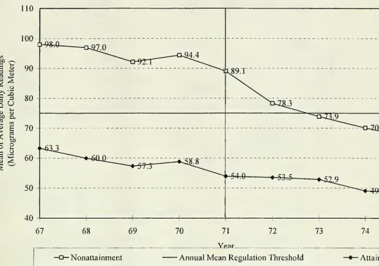
concentrations and housingprices. Figure

2A

examines the initial impact ofthe 1970

CAAAs

on

TSPs

concentrations.

The

counties with continuous monitorreadings

from

1967-1975 are stratified

by

theirregulatorystatus in 1972,

which

isthe firstyearthatthe

CAAAs

were

in force.22

The

horizontalline

at 75

pg/m

3 is the annual federal standard and the vertical line separates the pre-regulation years (1967

through 1971)

from

the years that the regulations

were

enforced.

The

exact

TSPs

concentration is

reportedateachdatapoint.

Beforethe

CAAAs,

TSPs

concentrationsare approximately 35

pg/m

3 higherinthenonattainment

counties.

The

pre-regulation time-seriespatterns ofthe

two

groups are virtually identical.

From

1971 to

1975,the setof 1972 nonattainment counties

had

astunning

22-pg/m

3reduction inTSPs, while

TSPs

fell

by

only 6

pg/m

3 in attainment counties, continuing their pre-1972 trend. This impliesthat virtually the

entirenationaldecline in

TSPs

from

1971-75 in Figure 1 isattributable to the regulations.

Figure

2B

demonstratesthat

mid-1970s

nonattainmentstatusis alsoassociatedwithreductions in

TSPs

concentrations. Here, countiesare divided into those thatarenonattainment in eitherorboth 1975

and 1976 and thosethat are attainmentin both years.

TSPs

concentrations forboth setsofcounties are

plotted for the years 1970-1980 for the

414

counties with readings in every year.

Average

TSPs

concentrations decline

by

approximately 17

pg/m

3 inboth setsofcounties

between

1970and 1974. This

is surprising since the 1975-6 nonattainmentcounties are

more

likely to be nonattainmentin 1972, but it

implies that, at least as it relates to pre-existing trends, the attainment counties

may

form

a valid

2

The sample consists of 228 counties with a total population of 89 million in 1970.

As

the Data Appendix

describes, 1972 nonattainmentstatusisdeterminedby1971 TSPsconcentrations.

counterfactual for the nonattainment ones.23 Specifically,

mean

reversion and differential trends are not

likely sources ofbias.

Between

1974 and 1980,

mean TSPs

concentrations declined

by

6.3

ug/m

3 in

nonattainment counties and increased

by

4.1

ug/m

3 in attainment counties. Consequently, mid-decade

nonattainmentstatusis associatedwitharoughly 10

ug/m

3relative

improvement

inTSPs.24 25

The

structure ofthe federal regulations lends itselfto the application of

two

validity tests ofthe

relationship

between

nonattainment status and changes in

TSPs

concentrations and housing prices.

Recall,nonattainment statusis a discrete functionofthe annualgeometric

mean

and secondhighest daily

concentrations of

TSPs

in the previous year.

The

first test is a comparison of the

outcomes

of

nonattainmentandattainment countieswithselectionyear

mean TSPs

concentrations "near"75

ug/m

3. If

the unobservables are similarat this regulatory thresholdthen a comparison ofthese nonattainment and

attainment countieswill control forall omitted factors correlatedwith TSPs. Thistesthasthe features of

a quasi-experimental regression-discontinuity design

(Cook

and

Campbell

1979).26

The

secondtest

compares

nonattainmentand attainment counties with selection year

mean TSPs

concentrations less than 75

ug/m

3. Here, the variation inregulatory status is based on violations ofthe

daily standard.

The

key assumption is that, conditional

on

selection year

mean

TSPs, the assignmentof

nonattainment status does not

depend

on

the potential outcome, or is "ignorable" (Rubin 1978). This

approachhasthe featuresofamatchingdesign.

23

73 ofthe 265 (117 ofthe 149) 1975-76 TSPs attainment(nonattainment) counties were TSPsnonattainment in

1972. Thus, over25percentofthe countiesswitchedtheirnonattainmentstatusbetweenthebeginning and middle ofthe decade.

24

Theresultsare qualitatively similar

when

Figure

2B

isbasedonthe988countiesinourprimarysample.

25

When

afiguresimilartoFigure

2B

isconstructed forthe 1980s,thereduction inTSPsattributabletomid-decade

regulations cannot be distinguished from differential responses to the 1981-82 recession. This finding is not

surprisinggiven thegeographic variation in the effect ofthe 1981-82 recession(Chay and Greenstone 2003b) and

theterminationoftheTSPsregulatoryprogramin 1987. For theseandothersreasons, this studyfocusessolely on the 1970s. Chay and Greenstone (1998) provide a fuller discussion ofthese issues and present the results from

strategies thataddresstheproblemsinestimatingthe

HPS

forthe 1980s.

2

In some contexts, leveraging a discontinuity design

may

accentuate selection biases ifeconomic agents

know

aboutthediscontinuitypoint and changetheirbehavioras aresult. Giventhewidevarietyoffactors thatdetermine

local

TSPs

concentrations ranging fromwind patterns to industrial output,

we

suspectthatcounties were unable to

engage in non-random sorting near the TSPs regulatory ceiling. Similarly

we

suspect that during the 1970s,

individualhomeownerswereunaware oftheproximity oftheircounty's

TSPs

concentrationtothe annualthreshold,

makingitunlikelythattheywould

move

as aconsequence.

Figure 3 graphically implements these checks

on

the validityof mid-decade

TSPs

nonattainment

status as an instrument. Separately for the 1975 attainment

and

nonattainment counties, each panel

graphs the bivariate relation

between

an

outcome

ofinterest and the geometric

mean

of

TSPs

levels in

1974, the selectionyear for the 1975 nonattainment designation.

The

plots

come

from

theestimation of

nonparametricregressionsthat use auniformkernel density regression smoother. Thus, they represent a

moving

averageofthe

raw

changes across 1974

TSPs

levels.27

The

difference inthe plots forattainment

and nonattainment counties can be interpreted as the impact of 1975 nonattainment status, both for the

counties exceedingjustthe daily concentration threshold (i.e., counties with 1974 concentrations

below

75

ug/m

3)andforthecountiesexceedingthe annualthreshold.

Panel

A

presents the 1970-80 change in

mean TSPs by

the level of

mean TSPs

in 1974. First,

compare

the nonattainment counties with selection year

TSPs

concentrations just

above

75

ug/m

3

(demarcated

by

the vertical line in the graph) and attainment counties just

below

this threshold.

The

figure reveals that right at the threshold nonattainment counties

had

an approximately 5

ug/m

3 larger

decline in

TSPs

than attainment counties over the course ofthe decade. Further an examination ofthe

counties withselection year

TSPs

concentration in the 65-85

ug/m

3 rangereveals that thenonattainment

counties

had

anywhere from

a 10-14

ug/m

3 greater reduction in

mean

TSPs.

The

size of the

TSPs

reductions declines forcountieswith 1974

mean

concentrations greaterthan90

ug/m

3. Further, the slight

downward

slopeinthe plot forattainment counties isconsistentwith

some

reversioninTSPs.

Second, consider the counties with annual

mean

concentrations

below

75 (J.g/m3. Here, the

nonattainment counties receivedthis designation forhaving as

few

as 2 "bad days". There are 67 such

counties.

A

comparison ofthesenonattainmentcounties to the attainment ones withselectionyear

mean

TSPs

concentrationsinthe

same

rangesuggests thatnonattainmentstatus isassociatedwithabouta5-unit

greaterreductionin

mean TSPs

overthedecade.28

27

The smoothedscatterplots are qualitatively similar for several differentchoices of bandwidth

-

e.g., bandwidths

thatusebetween 10to20percentofthedatatocalculate localmeans. !S

ThefindingfromFigures2and

3A

thatnonattainmentstatusisassociatedwith reductionsinTSPsconcentrations

contradictsrecentclaimsthattheClean AirAct had noeffectonairquality(Goklany 1999).

Panel

B

plots the conditional change in log-housing values

from

1970-80 separately for

nonattainmentandattainmentcounties.

Both

validitychecks indicateastrikingassociation

between

1975

nonattainment status and greater increases in property values over the decade.29

They

suggest that

nonattainmentcountieshad abouta0.02-0.04 log pointrelativeincreaseinhousingprices.

In

summary,

Figures 2 and 3

document

that nonattainment status is strongly associated with

reductions in

TSPs

and increases in housing prices.

The

discrete differences in

TSPs

changes and

housing price changes that are visible with the regression discontinuity and matching validity tests

provide convincingsupportfor a causal interpretationofthe effectof1975

TSPs

nonattainment status on

these outcomes.

Finally, Figure 3 foreshadows our results

on

the relationship

between

housing prices and TSPs.

In particular, the strongcorrespondence

between

the patterns in Panels

A

and

B

suggests that this

quasi-experiment

may

alsobe detecting a casualrelationship

between

airpollutionandproperty valuesthrough

the

mechanism

of regulation.

The

panels also imply that

MWTP

may

vary with the level of

TSPs

concentrations. Specifically, the ratio of the nonattainment-attainment difference in housing price

increases to thedifference in

mean TSPs

declinesislowerinmagnitudeindirtiercounties (i.e., thosewith

1974

TSPs

concentrations above 75

pg/m

3

).

One

explanation for this difference is that individualswith

strongpreferences forcleanair systematicallysorted to the relativelyclean areas. Inordertoexplore this

possibilityfurther, the

below

implementsan estimationapproachthatestimatestheaverage

MWTP,

while

attemptingtocontrol for sorting on heterogeneoustastes.

B.

Mid-Decade TSPs

NonattainmentStatus

There are theoretical andstatistical reasonsthatmid-decade (e.g., 1975-6)nonattainment statusis

a better candidate for an instrumental variable than the beginning of the decade nonattainment

designation. First, consider the theoretical rationale. Since annual county-level housing values are

29

Itshouldbenotedthatthere arenononattainment countieswith 1974geometric

mean TSPs

concentrationsbelow

40 pg/m3. Thecountieswith

mean

TSPsconcentrationsbelow40

pg/m

3

have

much

smaller populationsand

noticeablydifferent characteristicsfromthecountieswith higherTSPsconcentrations. Therefore, these counties

may

notbecomparabletotheothermonitoredcounties.

unavailable,

we

rely

on

1970 and 1980

Census

data. Additionally, Figures

2A

and

2B

suggestthat there

is atleast a 2-3 year lagbefore the full effects of

TSPs

nonattainment status

on

pollution reductionsare

realized.

A

focus

on

1972 nonattainment status

would

leave 5-6 years until the 1980 census,

which

is

likely

enough

time forindividuals to sortthemselvesinto

new

locationsand supplytorespond tothese air

qualitychanges. Consequently

when

housingprices are

measured

in 1980, thecomposition of people and

homes

may

differ

from

the composition in 1970. Inother

words

iflocal housing markets are integrated

overthis timehorizon, it

may

be invalid touse 1970-80 housingprice changesto

measure

the

MWTP

for

a reductionin

TSPs

inthe early 1970s.30

A

focus

on

mid-decade nonattainment status

may

mitigate this

problem

of compensatory

responses.

The

intuition is that the changes in air quality due to mid-decade regulation are not evident

until the end ofthe 1970s,

which

is roughly the

same

time that the

Census

Bureau

asks about housing

values. This

may

provide an opportunity to observe

how

TSPs

reductions are capitalized without

substantialcontamination

by

general equilibriumadjustments in

demand

and supply. Itis evidentthatthe

virtually identical "pre-period" change in

TSPs

concentrations in nonattainment

and

attainment counties

(recallFigure

2B)

is anecessary conditionforthis approachtobevalid.

The

second reason forourfocus

on

mid-decade

TSPs

nonattainmentstatusisthatthisdesignation

isuncorrected with

most

observabledeterminantsof housingprices, including

economic

shocks. Thisis

not true

when

comparing

beginning of decade nonattainment and attainment counties. Further,

we

find

evidence that there is likely to be substantial confounding in the conventional cross-sectional and fixed

effects approachestoestimating the

HPS.

Table2 presentsevidence

on

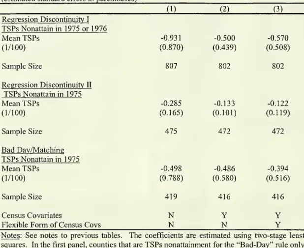
thesepoints.

Table 2

shows

the associationof

TSPs

levels,

TSPs

changes,and

TSPs

nonattainment statuswith

numerous

determinants of housing prices. In the first four columns, the sample is our base set of988

counties.

The

Column

5 entries are derived

from

our "regression discontinuity" sample of

475

counties

thatare near theannual threshold.

A

countyisincludedinthissample ifitmeets

two

criteria: 1) its 1974

geometric

mean TSPs

concentrations is in the 50-100

ug/m

3 range, and 2) ifits 1974 geometric

mean

,0

For example, Blanchard and Katz (1992) find that local housing prices fall in the first five years following a

negativelocal employment shockbut reboundfullywithinabout a decade oftheshock. This rebound inprices is

likelydueto thegeneralequilibriumresponsesofconsumers andsuppliersofhousing.

concentrationis

below

75 |J.g/m

3

, it

must

be designated attainment(i.e., allcountiesthatarenonattainment

solelydueto thebad day rule aredropped).

The

column

6 entries are

from

our

bad day

sample,

which

is

limitedtothe

419

countieswith 1974 geometric

mean

concentrations

between

50

and

75

ug/m

3.

The

entries in each

column

are the differences in the

means

ofthe variables across

two

sets of

countiesand the standard errorsofthe differences(inparentheses).

A

'*' indicates that the difference is

statistically significantatthe

5%

level, while '**' indicates significance at the

1%

level. If

TSPs

levels

were

randomly

assigned acrosscounties, one

would

expectvery

few

significant differences.

Column

1 presents the

mean

difference in the 1970 values ofthe covariates

between

counties

with 1970

TSPs

concentrations greater and less than the

median

1970 county-level

TSPs

concentration.

There are significant differences across the

two

sets of counties for several

key

variables, including

income

per capita, population, population density, urbanization rate, the poverty rate, the fraction of

housesthat are

owner

occupied, andtheshareof

government

spending on education. It is interesting that

mean

housing values are higher in the dirtier counties, although this difference is not statistically

significant at conventional levels.

Although

it is not presented here, an analogous examination ofthe

means

in 1980 leads to similar conclusions. Overall, these findings suggest that "conventional"

cross-sectional estimates

may

be biased dueto incorrect specification ofthe functional

form

ofthe observables

variablesand/oromittedvariables.

Column

2 performs a similaranalysis forthe 1970-1980

TSPs

changes. Here, the entries are the

mean

difference inthe change inthecovariates

between

counties with achange in

TSPs

that is less (i.e.,

larger declines) and greater than the

median

change in TSPs. Reductions in

TSPs

arehighly correlated

with

economic

shocks.

The

counties with largepollution declines experienced substantially less growth

in per-capita income, smaller population growth, a bigger increase in

unemployment

rates, a larger

decline in manufacturing employment, and less

new

home

construction. These entries demonstrate that

TSPs

concentrations are pro-cyclical and suggest that unless it is possible to perfectly control for the

economic

cycle,the fixed-effects estimatorofthe

HPS

willhavea positivebias. For example,the second

Column

3

compares

the 1970-80

change

in the

same

set of variables in 1970-2

TSPs

nonattainment and attainment counties. Here, a county is designated nonattainment if it exceeds the

federal standards in any of the years 1970, 1971, or 1972; all other counties are in the attainment

category.

The

nonattainmentcounties

had

a smaller increaseinper-capita

income growth

and larger

and

statistically significant declines in population, manufacturing

employment,

new home

construction,

and

populationdensity thantheattainmentcounties.

We

suspectthatthepopulationflowsreveal a substantial

worsening of

economic

conditions innonattainment counties. This worsening islikelyduetonon-neutral

impacts of the 1974-75 recession and/or the

economic

effects of the regulations themselves (e.g.,

Greenstone 2002). Just as with the fixed effects results, these entries suggestthat estimates thatrely

on

1970-2

TSPs

nonattainment status as an instrument

may

be positively biased due to the confounding of

changes in

economic

activity with the regulation-induced change in TSPs.

These

findings imply that

beginningof decade nonattainmentstatusisnotanattractivecandidate foraninstrumentalvariable.31

Columns

4

repeats this analysis

among

1975-6

TSPs

nonattainmentand attainment counties

and

finds that the observable determinants of housing prices are better balanced across these counties.

Remarkably, the mid-decade nonattainmentinstrumentpurges the non-neutral

economic

shocksapparent

above. For example,thedifferencesinthechangesinper-capitaincome, totalpopulation,

unemployment

rates, manufacturing

employment,

and

new

home

construction

among

the

two

sets ofcounties are all

smaller in magnitude than in the other

columns and

statistically indistinguishable

from

zero. Also,

nonattainment and attainment counties

had

almost identical changes in urbanization rates during the

1970s, suggesting that differential 'urban sprawl' within counties is not a source of bias.32 Notably,

nonattainmentcountieshad both agreaterreductionin

TSPs

andagreaterincreaseinhousingvalues

from

1970-80,foreshadowing ourinstrumental variableresults.

Finally,

columns

5 and 6

compare

the covariates across 1975

TSPs

nonattainment and attainment

counties fortheregression discontinuity and

bad

day samples. Itis evident thattheobservable variables

31

Countiesthatwere 1973-4TSPs nonattainmentalso hadstatistically significant largerdeclines inpopulation and

increasesinthepovertyrate. 32

Whilethere aresomesignificantdifferencesbetweennonattainmentandattainment countiesin 1970 valuesofthe

variables,thehypothesisofequal populationdensities in 1970cannotberejectedatconventionallevels.

are well balanced

by

nonattainment status in these columns. In fact,

none

of the

mean

differences in

column

5 arestatisticallydifferent

from

zero andonly

two

of

them

are in

column

6.33

Although a direct test ofthe validity ofthe exclusion restriction is as always unavailable, it is

reassuring that our instrumental variable is largelyuncorrectedwith observable determinants of housing

prices. Overall, the results in this table suggest that using mid-decade nonattainment status as an

instrumental variablehas

some

important advantages over "conventional" estimation strategies

and

also

overtheuseof beginning ofdecade nonattainmentstatusasaninstrumentalvariable.

Figure 4 provides a graphical overview ofthe location ofthe 1975-6

TSPs

nonattainment and

attainment counties.

A

county's shading indicates its regulatory status; light gray for attainment,black

fornonattainment, andwhite forthecountieswithout

TSPs

pollutionmonitors.

The

pervasiveness ofthe

regulatory

program

is evident. For example, 45 ofthe 51 states

had

at least one county designated

nonattainment. This is important if there are regional or state-specific determinants ofthe change in

housingprices

between

1970 and 1980.

In

summary,

there are severalreasons

why

ourapproachto estimatingthe

HPS

may

be attractive.

First,

TSPs

nonattainment status is strongly associated with large differential reductions in particulates

levels across counties.

The

timing and location ofthe changes provide convincing evidence that the

estimated pollutionimpact

may

be causal. Second, the nonattainmentdesignation islargely uncorrelated

with observable determinants of housing price changes, including

economic

shocks. In fact, the

instrument appears to purge the local

demand

and supply shocks that contaminate estimates based

on

'fixed-effects' analyses. Third, since the regulations are federally mandated, their imposition is

presumably orthogonal to underlying

economic

conditions andthe local politicalprocess determining the

supply ofnon-marketamenities.34

33

Further, thedifferencesinthe 1970levelsofthe variables are alsosmallerinthese restrictedsamples. Thisis

especially truein theregression discontinuity sample, wherethehypothesisofequalmeanscannotberejected forall

the covariates,except

%

Urban(p-value=.037).

34

Scientific evidence provides additional support for the credibility ofregulation instruments that depend on

pollution levels. Cleveland et al. (1976) and Cleveland and Graedel (1979) document that wind patterns often

transportairpollutionhundreds ofmilesandthattheozone concentrationofair entering intothe

New

Yorkregion

in the 1970s often exceeded the federal standards.

A

region's topographical features can also affect pollution

concentrations. Counties located in valleys (e.g., Los Angeles, Phoenix, Denver, the Utah Valley) are prone to

weatherinversionsthatlead toprolongedperiodsofhighTSPsconcentrations.

V.

Econometric

Models

forthe

HPS

and

Average

MWTP

Here,

we

discuss the econometric

models

used to estimate the hedonic price locus. First,

we

focus

on

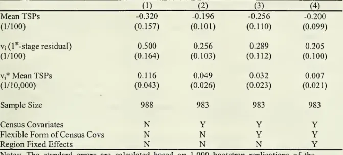
theconstantcoefficientsversion ofthese models.

We

then discuss a

random

coefficients

model

that allows for self-selection bias arising

from

taste sorting.

We

show

how

this

model

identifies the

average

MWTP

inthepopulationwhileproviding a simple statistical testofsortingbased

on

preferences

forclean air.

A. Estimationofthe

HPS

Gradient

The

cross-sectional

model

predominantly usedintheliteratureis:

(2) Yc70

=

Xc7o'P

+

6T

C70

+

Ec70, Ec70

=

0tc

+

Uc70

(3)

T

C70

=

X^o'II

+

T| C70, T| C70

=

A,c

+

V

c70,

where

_yc70 is the log of the

median

property value in county c in 1970,

X

_c70 is a vector

of

observed

characteristics,

T

_{c70 is}thegeometric

mean

of

TSPs

across all monitors inthecounty, ands_c70

and

r\_c70 are

theunobservable determinantsof housing pricesand

TSPs

levels, respectively.35

The

coefficientG is the

'true' effect of

TSPs

on

properly values and is interpreted as the average gradient ofthe

HPS.

For

consistent estimation, the least squares estimator of 9 requires E[sc7oqC7o]

=

0. If there are omitted

permanent (ac and

X

c) ortransitory(u^o

and v

c70) factors that covary with both

TSPs

and housing prices,

thenthe cross-sectionalestimatorwillbebiased.

With

repeated observations over time, a 'fixed-effects'

model

implies that first-differencingthe

datawillabsorb thecounty

permanent

effects,

a

cand A. c. This leadsto:

(4)

y

G80 -

y

C70

=

(Xcso-_Xc7o)'P

+

6(T

_c80-

T

_c70)

+

(U_c80-Uc7o)

(5)

T

c8o-

T

c70

=

(Xcso-Xc7o)'Il

+

(vc80-

V

c70).

35

For each county,

T

c70 (Tc8o) is calculated as the average across the county's annual

mean

TSPs concentrations

from 1969-72 (1977-80). Eachcounty's annual

mean

TSPs concentrationistheweightedaverageofthe geometric

mean

concentration of each monitor in the county, using the number of observations per monitor as weights.

Averagingovermorethanoneyearreducestheimpact of temporaryperturbations onourmeasures ofpollution.

Foridentification,theleast squares estimatorof9 requires E[(uC8o-uc70)(vc80

- v

c70)]=0. That is,there are

no

unobserved shocks topollutionlevels thatcovary with unobserved shocks tohousingprices.

Suppose

there is aninstrumental variable (IV),

Z

c, that causes changes in

TSPs

without havinga

direct effect

on

housingpricechanges.

One

plausibleinstrumentismid-1970s

TSPs

regulation,

measured

by

theattainment-nonattainment statusofa county. Here,equation (5)becomes:

(6)

T

c80-

T

c70

=

(Xc80-

X

c7o)'nTx

+

Z^Efe

+

(vc8o-vc70) ,and

(7)

Z

c75

=

l(Tc74

>

T

)

=

1(vc74

>

T

-

Xc

74

'n

-

X

c),

where

Z

c75 is the regulatory status of county c in 1975, 1(») is an indicatorfunction equal to one ifthe

enclosed statement is true, and

T

is the

maximum

concentration of

TSPs

allowed

by

the federal

regulations.36 Nonattainment status in 1975 is a discrete function of

TSPs

concentrations in 1974. In

particular, if

T^

and

T

_c

™

x

are the annual geometric

mean

and 2nd highest daily

TSPs

concentrations,

respectively,thenthe actualregulatory instrumentused is

l(T

c a 7|

>

75

ug/m

3 or

T

c

™

x

>

260

ug/m

3).

An

attractive feature ofthis approach is that the reduced-form relations are policy relevant. In

particular,

n

Tz

from

equation (6) measures the change in

TSPs

concentrations innonattainment counties

relativetoattainment ones. In theotherreduced-formequation,

(8) Vc80-_yc70

=

(Xc80"

X

_c7o)TIyX

+

Z

c75llyz

+

(ucso-Uc70 )°,

n

yZcapturesthe relativechange inlog-housingprices. Sincethe

IV

estimator, (9iV),is exactly identified,

itisa simpleratioofthe

two

reducedformparameters,thatis 8iV

=

n

yz/nTz.

Two

sufficient conditions forthe

IV

estimator (9iV) toprovide a consistent estimate ofthe

HPS

gradientare

H

_TZ

*

and

E[v

c74(uc8o- uc70 )]

=

0.

The

firstconditionclearly holds.

The

second condition

requires that unobserved price shocks from 1970-80 are orthogonal to transitory shocks to 1974

TSPs

levels. Inthe simplestcase,the

TV

estimatorisconsistentif

E[Z

c75(uc8o-Uc70)]

=

0.

We

implement

the

IV

estimatorin a

number

of ways. First,

we

use all ofthe available data and

themid-decade nonattainmentindicator as the instrumentto obtain9IV.

We

alsocalculate

IV

estimatesin

two

other

ways

that allow forthe possibility that E[vc74(uc80-

u

c70 )]

^

overthe entire sample.

The

first

36

In practice, our preferred instrument equals 1 ifacounty is nonattainmentin 1975 or 1976 and otherwise. In

thissection,

we

denoteitwith

Z

c75foreaseofexposition.