Dissolution in a porous rock: effect on the concentration–discharge relationships

HAL Id: hal-01501292

https://hal-univ-paris.archives-ouvertes.fr/hal-01501292

HAL is a multi-disciplinary open access archive for the deposit and dissemination of sci-entific research documents, whether they are pub-lished or not. The documents may come from teaching and research institutions in France or abroad, or from public or private research centers.

L’archive ouverte pluridisciplinaire HAL, est destinée au dépôt et à la diffusion de documents scientifiques de niveau recherche, publiés ou non, émanant des établissements d’enseignement et de recherche français ou étrangers, des laboratoires publics ou privés.

Dissolution in a porous rock: effect on the

concentration–discharge relationships

O Devauchelle, F Métivier, E Lajeunesse, J Gaillardet, J.F. Didon, Youcun

Liu, Baisheng Ye

To cite this version:

O Devauchelle, F Métivier, E Lajeunesse, J Gaillardet, J.F. Didon, et al.. Dissolution in a porous rock: effect on the concentration–discharge relationships. River, Coastal and Estuarine Morphodynamics, 2011, Beijing, China. �hal-01501292�

River, Coastal and Estuarine Morphodynamics: RCEM2011 © 2011 Tsinghua University Press, Beijing

Dissolution in a porous rock: effect on the concentration–discharge

relationships

Olivier DEVAUCHELLE, François METIVIER, Éric LAJEUNESSE,

Jérôme GAILLARDET

Équipe de dynamique des Fluides Géologiques

Institut de Physique du Globe de Paris Sorbonne Paris Cité Université Paris Diderot, UMR 7154 CNRS

1 rue Jussieu, 75238 Paris cedex 05, France

Jean-François DIDON-LESCOT

UMR 6012 ESPACE

Avenue du Général de Gaulle, 30380 Saint-Christol-les-Alès, France

LIU Youcun

Key Laboratory of Water Environment and Resource, Tianjin Normal University 393 Binshui west road, Tianjin 300387, China

YE Baisheng

States Key Laboratory of Cryospheric Science

Cold and Arid Regions Environmental and Engineering and Research Institute Chinese Academy of Sciences, 260 Donggang West road, Lanzhou, China

ABSTRACT: Various empirical or physically-based theory have been proposed to understand how the solute concentration of a stream varies with the discharge. We focus here on the influence of the dynamics of the groundwater flow on the chemical erosion rate. To do so, we couple a one-dimensional aquifer model to a first order dissolution equation. If the aquifer extends far below the stream level, the theoretical discharge–concentration equation corresponds to the empirical “working model” proposed by Johnson in 1969, thus providing a physical interpretation of its parameters. Conversely, if the aquifer lays mainly above the stream level, a significantly different relationship is found. These theoretical findings are then compared to two field-data sets. From this comparison, we conclude that the dynamics of the groundwater flow could play a significant role in moderating the impact of dilution on the stream concentration at large discharges.

1 INTRODUCTION

In order to assess the chemical erosion rate of a catchment from solute transport in rivers, one needs to know both the statistical properties of the hydrograph, and the concentration of the various solutes as a function of water discharge. We focus here on the second question.

The most direct way to evaluate the concentration–discharge relationship of a given catchment is through the continuous measurement of the two quantities over a sufficiently long period of time (Hem 1948). Typically, one finds that the concentration in major ions c decreases as the stream discharge Q increases, although more slowly than 1/Q (Godsey et al. 2009). Since the total solute flux is the product of

794

stream discharge with the concentration, this empirical finding indicates that the solute flux increases with discharge, and consequently that extreme flood events can have a major influence on the average chemical weathering rate (Calmels et al. 2011; Liu et al. 2011). When this is true, it is necessary to represent correctly the asymptotic behavior of the concentration at high discharges. Unfortunately, extreme events are difficult to monitor, due to obvious technical reasons associated to the scarcity of such events in the record.

In order to extrapolate the concentration–discharge relationship beyond the available data range, one needs to understand the chemical and physical processes which control the solute concentration. The first theories, initiated by Johnson et al. (1969), were based on the mixing of two volumes of water of different concentrations (for instance, rain water with soil water). Assuming the stream discharge is proportional to the volume of water stored in a reservoir, one finds the so called “working model”,

(1) where a, b and d are parameters to be adjusted to field data. The working model is versatile enough to fit a large variety of data set. However, the physical interpretation of its parameters is controversial (Godsey et al. 2009). Also, its dilution-like behavior at large discharge (when a vanishes), is often considered unrealistic.

To address this limitation, Langbein and Dawdy (1964) introduced non-linear dissolution kinetics in their model. The order of the rock dissolution reaction is then a free parameter capable of representing the departure of concentration–discharge relationships from simple dilution. Godsey et al. (2009) explain differently the near-chemostatic behavior of concentration–discharge relationships. Their model is based on the existence of vertical gradient of porosity, permeability and pore aperture. As the groundwater flux towards the stream varies, the elevation of the water table adjusts to the amount of water the aquifer needs to carry, and consequently explores the vertical profile of physical properties of the rock. Under simplifying assumptions, Godsey et al. (2009) can relate the exponent of the concentration – discharge relationship to the characteristic lengths of the rock properties profiles. An essential distinction between the model of Godsey et al. (2009) and the more heuristic working model is that it involve physical quantities which can be evaluated independently from the concentration prediction itself, thus providing more confidence in the extrapolation at large discharges.

The present paper focus on the effect of the aquifer deformation on the water concentration, as the precipitation rate varies. This geometrical effect differs from the mechanism invoked by Godsey et al. (2009) in that we consider a homogeneous rock in which the shape of the water table itself influences the dissolution process. We stress here that the present contribution aims at isolating a specific mechanism, rather than combining all the mechanisms known to influence the concentration in order to make direct predictions in a specific catchment. Our hope is that the analysis of an isolated phenomenon can help us identify it in field data.

2 AQUIFER MODEL 2.1 Assumptions

Let us consider an aquifer laying in a homogeneous layer of porous rock (see figure 1). The vertical distance between the impervious boundary and the water table is named h. We assume that the dissolution of the solute of interest occurs within the bulk of the aquifer, thus neglecting both the dissolution occurring in the unsaturated ground above the water table, and any vertical variation of the physical and chemical properties of the rock.

If the horizontal dimension (of order L, the distance between the river and the water divide) is much larger than the typical thickness of the aquifer, then the so-called Dupuit approximation holds, and the behavior of the aquifer can be reduced to the horizontal dimension x (Dupuit 1863). This hypothesis is often valid in the field (Petroff et al. 2011). In accordance with this classical approximation, we will consider that the aquifer is sufficiently well-mixed vertically to define a concentration field c which depends only on the distance from the divide x.

We consider only slow variations of the precipitation intensity, so that the aquifer is always at equilibrium with the average rainfall. We thus neglect any hysteresis in the concentration–discharge

relationship. Finally, the chemical processes are reduced to a first-order dissolution reaction, characterized by a dissolution time T and the saturated concentration of the rock cs.

2.2 Groundwater flow

In a rock of permeability k, Darcy’s law reads

(2) where u,  and p are the water velocity, its dynamic viscosity and the pressure gradient respectively

(Darcy (1856). If the water-table surface is almost flat, the flow is essentially confined in the horizontal plane, and the pressure field is almost hydrostatic (Dupuit’s approximation). The vertically integrated flux of water q in the horizontal x direction reads

(3) where the conductivity K is defined as K =kg/ ( is the density of water).

Let R be the rainfall rate, uniform in space and constant in time. The mass balance for water then leads to the Poisson equation:

(4) The flux of water vanishes at the water divide, q(0) = 0, and the elevation of the water table equals the elevation of the river at the seepage face, h(L) = hr. Consequently, the solution to the Poisson equation is

(5) Figure 1 presents an example of water table profile. The rainfall R (and thus the river discharge) controls not only the water flux q but also the thickness h of the aquifer. The next section is devoted to the influence of both quantities on the groundwater concentration.

Figure 1 Schematics of an aquifer, and associated notations. The rainfall water fills the aquifer, which in turns flows into a stream. The porous rock is dissolved by groundwater, the concentration of which depends on the shape h(x) of the aquifer

2.3 Mass balance for the solute

The solute concentration in rainwater is named cr, and its concentration in the aquifer is c. Assuming a

first-order dissolution equation with rate 1/T, the solute mass balance reads

(6) In the above equation, the first term corresponds to the quantity of solute rainwater brings into the aquifer. The second term represents the solute advection by groundwater, and the last term corresponds to

796

the first-order dissolution process. Let us define the non-dimensional concentration c and the

non-dimensional horizontal coordinate X as follows

(7) Then equation (6) becomes

(8) where we have introduced the dimensionless rainfall rate P and the dimensionless aquifer thickness H,

(9) At the divide, the derivative of the concentration must remain finite. Equation (8) thus imposes

(10) As visible on Figure 2, the solution to equation (8) depends strongly on the dimensionless rainfall rate P. As expected, when the characteristic dissolution time is much longer that the typical time of travel through the aquifer (P≫1), the concentration tends towards the rainfall concentration cr. Conversely, for

fast dissolution (P≪1), the concentration tends toward the saturation concentration of the rock cs. The

river elevation with respect to the impervious layer, embedded in the parameter H, has a more intricate effect, which we describe in the next section.

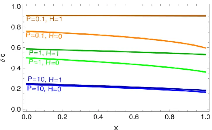
Figure 2 Distribution of the non-dimensional solute concentration along an aquifer, for various values of the parameters defined in relation (9). The water divide is at X=0, whereas X=1 corresponds to the aquifer outlet into the river

2.4 Theoretical concentration–discharge relationship 2.4.1 General solution

For an arbitrary set of dimensionless parameters P and H, one can approximate numerically the solution to equation (8) and its associated boundary condition (10). Assuming permanent regime, the value of the concentration profile at the aquifer outlet, that is at X=1, is the concentration in the river itself. Similarly, the river discharge is

Q =R L Lr (11)

where Lr is the length of the river upstream of the measurement point (L Lr is the drainage area associated

to this point). Consequently, the shape of the concentration–discharge relationship is the plot of co

versus P=T2KQ/(L3Lr).

discharge tends toward the rock saturation concentration cs, whereas for high discharge the river

concentration tends towards the rain concentration. The next sections are devoted to the asymptotic behavior of this relationship at intermediate rainfall rates.

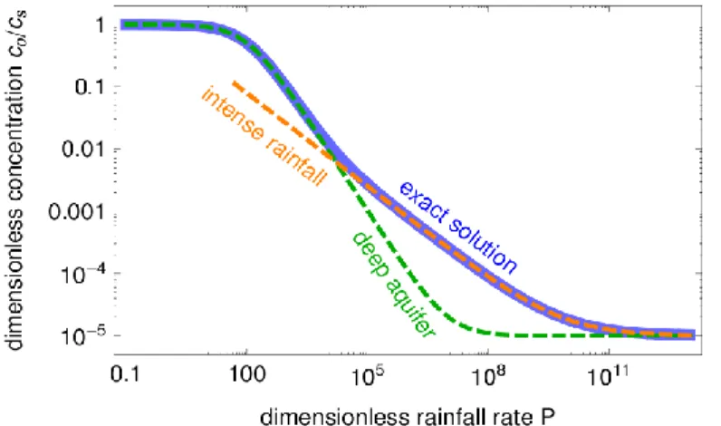
Figure 3 Theoretical concentration-discharge relationships for H=100 and cr/cs=10-5. The complete

solution requires the numerical integration of equation (8), whereas the two asymptotic behaviors correspond to the analytic expressions (13) and (20)

2.4.2 Deep aquifer

The aquifer can be considered deep when the variation in its elevation has a negligible influence on the thickness of the aquifer, although it still controls the hydrostatic pressure that drives the flow. In equation (8), it translates into H2≫P:

(12) The above equation, together with its boundary condition (10) admits the constant solution

(13) Returning to dimensional quantities, the above solution reads

(14) where co is the concentration at the aquifer outlet (Figure 3). The above equation corresponds exactly to

the working model, although the present model suggests a new interpretation for the relationship introduced by Johnson et al. (1969). Of course, interpretations are indistinguishable from each other by means of discharge and concentration measurements only. However, the parameters cs, cr, T and hr can in

principle be measured independently in the field. It is remarkable that, as long as the deep aquifer approximation holds, the ground permeability k is absent from relation (14).

2.4.3 Shallow aquifer

We call shallow aquifer the case in which the river flows directly on the impervious layer (H=0). This case maximizes the curvature of the aquifer, and thus the effect of its geometry on rock dissolution. Using the variation of constants method, equation (8) and its boundary condition (10) impose, at the river

(15) In terms of dimensional quantities, the outlet concentration reads

798

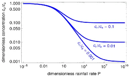
(16) The above equation represents a concentration-discharge relationship qualitatively similar to the working model, except at intermediate rainfall rates, where the concentration scales like 1/R1/2 instead of 1/R (Figure 4).

Figure 4 Theoretical concentration-discharge relationships for a shallow aquifer (H=0). The graphs correspond to relation (16)

2.4.4 Intense rainfall

The solution to the dissolution equation (8) can also be approximated when the the rainfall rate tends to infinity. More specifically, we assume now that P≫1 while H remains fixed. Accordingly, we expand the concentration up to first order in 1/P1/2,

(17) Equation (8) then requires

(18) and the boundary condition (10) becomes

(19) Equation (18) has an analytical solution, and for large rainfall rates the concentration can be approximated by

(20) Finally, returning to dimensional quantities, the concentration at the aquifer outlet reads

(21) As expected, for large rainfall rates, the concentration in the stream tends towards cr, the rain

concentration (Figure 3). However, at intermediate rainfall rates the concentration decreases as 1/R1/2, thus more slowly than simple dilution would.

3 COMPARISON WITH FIELD DATA AND DISCUSSIONS

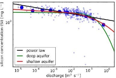
Concentration–discharge relationships are often close to chemostatic behavior (Godsey et al. 2009). Naturally, the aquifer model can represent this behavior, since the concentration in the aquifer tends to the saturation concentration when the typical residence time in the aquifer becomes long as compared to the dissolution time (P≪1). In order to illustrate how the influence of the aquifer geometry could be identified in the field, we have selected two data sets showing a clearly non-chemostatic behavior. The first data set was collected in the Ürümqi river in China, which flows in glacial moraines on the north flank of the Eastern Tianshan range (Liu et al. 2008). The sampling site is located 8 km downstream of the source, at an elevation of 3300 m. Its hydrology is controlled mainly by summer orographic precipitation, and the melting of the upstream glacier. The average discharge is about 1.2 m3s-1 (Métivier et al. 2004).

Figure 5 shows the measured concentration–discharge relationships for Silicon in the Ürümqi river. We then compare it to two limit cases of the aquifer model (shallow and deep), as well as to a power-law which prefactor and exponent are fitted to the data, for illustrative purposes. Assuming a vanishingly small concentration of atmospheric water in major ions (cr=0), the theoretical concentration–discharge

relationships are characterized by two parameters, namely the saturation concentration cs and a

characteristic discharge Qc. For a deep aquifer Qc =L Lr hr/T , after relations (11) and (14). For a shallow

aquifer Qc =L3Lr hr/(T2K), after relations (11) and (16). Graphically in the log-log plane, fitting the aquifer

model to data consists in shifting a curve along the concentration and discharge axes, without changing its shape. The data from the Ürümqi river show a strong negative correlation between discharge and concentration, but no significant curvature of the relationship. Consequently, it is not possible to discriminate between a power-law and any of the asymptotic behavior of the aquifer model. In order to do so from concentration measurements only, one would need to acquire data over a wider range of discharges.

Figure 5 Concentration of Silicon as a function of discharge in the Ürümqi River, China (small blue dots). All three models have two adjustable parameters. Power-law: c =1.7Q-0.34 (if c and Q are expressed in mgL-1 and m3s-1 respectively); deep aquifer: cs=2.2 mgL

-1

and Qc =3.3 m 3

s-1 ; shallow aquifer: cs=5.1 mgL-1 and Qc =0.45 m3s-1. The large blue dots represent bin averaged data

The second data set was collected in a 54 ha catchment of the Mont-Lozère, part of the granitic Cévennes mountains in France (Marc et al. 2001). The sampling site is located at about 500 m from the spring, and about 1150 m above sea level. The rainfall rate shows strong seasonal variations, with large storm events in autumn and spring, and dry summers and winters. The average discharge is about 21.4 m3s-1.

Figure 6 shows the concentration–discharge relationships for Silicon in the Mont-Lozère stream. The data span over five orders of magnitude in discharge, thus showing a significant curvature in the concentration–discharge relationship. This curvature is well represented by the shallow aquifer limit, whereas the deep aquifer approximation leads to an excessively curved relationship.

800

Figure 6 Concentration of Silicon as a function of discharge in a stream of the Mont Lozère, France (small blue dots). All three models have two adjustable parameters. Power-law: c=1.1Q-0.05 (if c and Q are expressed in mgL-1 and m3s-1 respectively); deep aquifer: cs=1.5 mgL-1 and Qc =0.65 m3s-1; shallow

aquifer: cs=1.7 mgL -1

and Qc =2.2 m 3

s-1. The large blue dots represent bin averaged data

4 CONCLUSIONS

A simple aquifer model coupling the basic geometrical properties of the aquifer to a first-order dissolution produces a rich variety of concentration–discharge relationships. It is capable of reproducing the near-chemostatic behavior of many field-data sets, as well as the curvature of the relationship measured by Marc et al. (2001). We certainly do not claim that the geometry of the aquifer dominates any other mechanism such as the influence of rock-property gradients, or more complicated chemical processes (e.g. higher order dissolution or re-precipitation). However, the present work suggests that the physics of groundwater flow could strongly influence chemical erosion rates.

Concentration–discharge relationships, by themselves, can hardly discriminate between the various regimes of groundwater flow. We believe a fortiori that they are not sufficient to discriminate between theories. Consequently, they should be complemented by other field measurements, performed on the same catchment. For instance, one could evaluate the physical quantities involved in the parameters of the present model independently, such as the ground conductivity, the dimensions of the aquifer or the chemical constants of the dissolution reaction. The next step would be to measure other quantities that are predicted by the theory, such as the spacial distribution of concentrations in groundwater. Also, as recommended by Godsey et al. (2009), one should check that the values of the physical quantities of a given catchment need not be adjusted to reproduce the concentration–discharge relationship for distinct solutes.

5 ACKNOWLEDGEMENTS

This is contribution # 3170 of the Institut de Physique du Globe de Paris. REFERENCES

Calmels, D., Galy, A., Hovius, N., Bickle, M., West, A. J., Chen, M.-C., and Chapman, H. (2011). Contribution of deep groundwater to the weathering budget in a rapidly eroding mountain belt, taiwan. Earth and Planetary Science Letters, 303(1-2):48.

Darcy, H. (1856). Les fontaines publiques de la ville de Dijon. Dalmont.

Dupuit, J. (1863). Études théoriques et pratiques sur le mouvement des eaux dans les canaux découverts et à travers les terrains perméables. Dunod.

Godsey, S. E., Kirchner, J. W., and Clow, D. W. (2009). Concentration-discharge relationships reflect chemostatic characteristics of us catchments. Hydrological Processes, 23(13):1844.

Hem, J. D. (1948). Fluctuations in concentration of dissolved solids of some southwestern streams. Transactions, American Geophysical Union, 29(1):80–84.

Johnson, N. M., Likens, G. E., Bormann, F. H., Fisher, D. W., and Pierce, R. S. (1969). A working model for the variation in stream water chemistry at the hubbard brook experimental forest, new hampshire. Water Resources Research, 5(6):1353–1363.

Langbein, W. B. and Dawdy, D. R. (1964). Occurrence of dissolved solids in surface waters in the united states. USGS Prof. Pap. 501-D, 115.

Liu, Y., Métivier, F., Gaillardet, J., Ye, B., Meunier, P., Narteau, C., Lajeunesse, E., Han, T., and Malverti, L. (2011). Erosion rates deduced from seasonal mass balance along an active braided river in tianshan. In preparation for Solid Earth Discuss.

Liu, Y., Métivier, F., Lajeunesse, E., Lancien, P., Narteau, C., Ye, B., and Meunier, P. (2008). Measuring bedload in gravel-bed mountain rivers: averaging methods and sampling strategies. Geodinamica Acta, 21(1-2):81.

Marc, V., Didon-Lescot, J. F., and Michael, C. (2001). Investigation of the hydrological processes using chemical and isotopic tracers in a small mediterranean forested catchment during autumn recharge. Journal of Hydrology, 247(3-4):215–229.

Métivier, F., Meunier, P., Moreira, M., Crave, A., Chaduteau, C., Ye, B., and Liu, G. (2004). Transport dynamics and morphology of a high mountain stream during the peak flow season: the ürümqi river (chinese tian shan). 1:761–777.

Petroff, A. P., Devauchelle, O., Abrams, D. M., Lobkovsky, A. E., Kudrolli, A., and Rothman, D. H. (2011). Geometry of valley growth. Journal of Fluid Mechanics, page 1.