HAL Id: hal-00697578
https://hal-enpc.archives-ouvertes.fr/hal-00697578
Submitted on 22 May 2012
HAL is a multi-disciplinary open access
archive for the deposit and dissemination of
sci-entific research documents, whether they are
pub-lished or not. The documents may come from
teaching and research institutions in France or
abroad, or from public or private research centers.
L’archive ouverte pluridisciplinaire HAL, est
destinée au dépôt et à la diffusion de documents
scientifiques de niveau recherche, publiés ou non,
émanant des établissements d’enseignement et de
recherche français ou étrangers, des laboratoires
publics ou privés.
invariance, a theoretical reply
D Schertzer, Ioulia Tchiguirinskaia, S. Lovejoy, A. F. Tuck
To cite this version:
D Schertzer, Ioulia Tchiguirinskaia, S. Lovejoy, A. F. Tuck. Quasi-geostrophic turbulence and
general-ized scale invariance, a theoretical reply. Atmospheric Chemistry and Physics, European Geosciences
Union, 2012, 12 (1), pp.327-336. �10.5194/acp-12-327-2012�. �hal-00697578�
Atmos. Chem. Phys., 12, 327–336, 2012 www.atmos-chem-phys.net/12/327/2012/ doi:10.5194/acp-12-327-2012
© Author(s) 2012. CC Attribution 3.0 License.
Atmospheric
Chemistry
and Physics
Quasi-geostrophic turbulence and generalized scale invariance, a
theoretical reply
D. Schertzer1, I. Tchiguirinskaia1, S. Lovejoy2, and A. F. Tuck1
1Universit´e Paris-Est, Ecole des Ponts ParisTech, LEESU, Marne-la-Vall´ee, France 2McGill U., Physics dept, Montreal, Canada
Correspondence to: D. Schertzer ([email protected])
Received: 23 November 2010 – Published in Atmos. Chem. Phys. Discuss.: 31 January 2011 Revised: 21 December 2011 – Accepted: 21 December 2011 – Published: 5 January 2012
Abstract. Lindborg et al. (2010) claim that the apparent
spectrum power law E(k) ≈ k−3 on scales ≥ 600 km ob-tained with the help of commercial jetliner trajectory devi-ations (GASP and Mozaic databases) could not be brought into question (Lovejoy et al., 2009a), because this spectrum corresponds to “a well known theory of quasi-geostrophic turbulence developed by Charney (1971)”. Lindborg et al. (2010) also claim that “limitations [of this theory] have been relaxed in many of the modern models of atmospheric turbu-lence”. We show that both claims are irrelevant and that gen-eralized scale invariance (GSI) is indispensable to go beyond the quasi-geostrophic limitations, to go in fact from scale analysis to scaling analysis in order to derive better analyt-ical models. In this direction, we derive vorticity equations in a space of (fractal) dimension D = 2 + Hz (0 ≤ Hz≤1),
which corresponds to a first step in the derivation of a dy-namical alternative to the quasi-geostrophic approximation and turbulence. The corresponding precise definition of frac-tional dimensional turbulence already demonstrates that the classical 2-D and 3-D turbulence are not the main options to understand atmospheric dynamics. Although (2+Hz)-D
tur-bulence (with 0 < Hz< 1) has more common features with
3-D turbulence than with 2-D turbulence, it has nevertheless very distinctive features: its scaling anisotropy is in agree-ment with the layered pancake structure, which is typical of rotating and stratified turbulence but not of the classical 3-D turbulence.
1 Introduction
The scale analysis methodology developed by Charney (1948) in his seminal derivation of the quasi-geostrophic (QG) approximation has become standard in meteorology and oceanography (Pedlosky, 1979). Unfortunately, its com-mon and distinguishing features with respect to a scaling analysis have not yet been fully recognized. It is ironical that the source of the present debate on intermediate scale at-mospheric dynamics presumably corresponds to the impor-tation into meteorology of two successive techniques from hydrodynamics at two different periods. In order to focus the present paper on this question and therefore on the lim-itations of the theory of quasi-geostrophic turbulence (QGT, Charney, 1971) and show how to overcome them, let us first reject the second claim of Lindborg et al. (2010), LT-NCG hereafter, that models may overcome limitations of a theory because in a very general manner models are ob-tained by introducing further constraints into a given the-oretical framework, e.g. boundary conditions, discretiza-tion of partial differential equadiscretiza-tions, subgrid modelling and other parametrizations. Furthermore, these constraints in the unique quasi-geostrophic model simulation (Tung and Or-lando, 2003) cited by LTNCG were such a problem that, as discussed below, they seem to have introduced spurious nu-merical estimates of the scaling ranges, instead of relaxing limitations of the theory.
Before addressing QGT, we will first discuss a few fun-damental features of the derivation of the QG approxima-tion itself, as well as its motivaapproxima-tion. This detailed discus-sion (Sect. 2) is necessary (i) to better evaluate the limita-tions of quasi-geostrophic turbulence (QGT, Sect. 3) and (ii) to enable us to derive an alternative (Sect. 4). In particular,
we show that to better understand the fundamentals of atmo-spheric dynamics a scaling analysis is required instead of a scale analysis, which was the basic technique used by Char-ney in his derivation and led to a drastic reduction of vortex stretching. Both questions are discussed throughout our pa-per and they enable us to obtain in a straightforward man-ner a vorticity equation for a turbulence that at first glance looks two-dimensional at large scales, three-dimensional at small scales, but is in fact of (fractal) dimension D = 2 + Hz
(0 ≤ Hz≤1) at all scales as illustrated by Fig. 1. We believe
that this equation may satisfy those who asked for a dynam-ical alternative to QGT (Yano, 2010), although this should be completed by a similar treatment of the thermodynamic energy evolution equation.
As our paper is already long, we prefer to acknowledge the necessity of this second step rather than to proceed with it. It may be helpful to note that this paper does correspond to a reply to the comment issued by LTNCG on the paper of Lovejoy et al. (2009a), LTSH hereafter. However, because the debate with LTNCG bears on very fundamental issues and not on technical details this yielded a stand alone pa-per that has many more original results (e.g. new dynamical equations, as well an original technique to derive them) than a usual reply to a comment. As mentioned in the title, it is a “theoretical reply”, because it is focused on theory, not on the empirical evidence brought by LTSH that the empirical spectral slope value is closer to 2.2 (as for buoyancy sub-range) than to 3 (as for the enstrophy (i.e. square vorticity) inertial subrange of 2-D turbulence) and could correspond to the fact that aircraft sample the vertical fluctuations instead of the horizontal ones. The present paper is indeed focused on the dynamical/physical modelling of these observations.
2 QG vorticity equation and scale analysis
Before discussing the derivation of the QG approximation, let us highlight why this approximation has remained so at-tractive and therefore popular. Historically, it was the first mathematically self-consistent derivation of a closed dynam-ical system from the diagnostic geostrophic and hydrostatic approximations. It also respects the conservation laws of po-tential temperature and absolute popo-tential vorticity, at least their corresponding first order expressions within the QG ap-proximation. Furthermore, the global mathematical proper-ties (e.g. for large times) of QG solutions are known, unlike those of the Navier-Stokes equations, as well as the fact that exact results were obtained on their order of approximation with respect to the primitive equations (PE) with rather mild restrictions on the initial conditions (Bourgeois and Beale, 1994). However, PE correspond already to a given set of ap-proximations (e.g. inviscid, incompressible flow with vari-able density, Boussinesq and (quasi-) hydrostatic assump-tions, (Pedlosky, 1979) for discussion), which can be brought into question on various ranges of scale.
Fig. 1. Vertical cut of the average eddies -more precisely: average iso-contours of the horizontal velocity fluctuations- of a turbulence in a space of (fractal) dimension D = 2+Hz(0 ≤ Hz≤1) (here with the theoretical value Hz=5/9, see text). The largest structures are flattened along the horizontal in agreement with the layered pan-cake structure, which is typical of rotating and stratified turbulence, but remain distinct from 2-D structures.This flattening is more pro-nounced for lower and lower values of Hz.
Let us also recall that the derivation by Charney (1948) of the QG approximation was based on a scale analysis, bor-rowed from aerodynamic boundary layer theory (Charney refers to Goldstein, 1938) to intentionally filter out the teorologically insignificant wave components” from the “me-teorologically significant motions”. The latter were consid-ered to be distinguishable from all other types of atmospheric motion only by a great difference in scales. This question of filtering was essential for the sake of the pioneering de-velopment of numerical weather forecasting (Charney et al., 1950) and a part of the paper by Charney (1948) was indeed devoted to checking that this filtering was efficient for acous-tic waves. Nevertheless, the more general question of which structures were filtered out was not addressed. Another im-portant requirement put forward by Charney was also related to numerical forecasts: the approximation should be (easily) computable. It is worthwhile noting that none of these is-sues is related to the question of obtaining a rather complete description of the atmospheric dynamics.
More precisely, the scale analysis performed by Char-ney was based on the common idea in meteorological prac-tice that large scale dynamics were quasi-two-dimensional, quasi-geostrophic and quasi-hydrostatic, due to the fact that the rotation and the gravitational field g of the Earth intro-duce preferential directions in the Navier-Stokes equations:
Du/Dt + 2 × u = −∇p/ρ + g + ν1u (1)
where u is the velocity, p the pressure, ρ the density, ν the viscosity, D/Dt denotes the material derivative, i.e. the time derivative following the motion (∂/∂t + u · ∇), ∇ denotes the 3-D gradient operator, 1 = ∇2the 3-D Laplace operator. The velocity field is assumed to be solenoidal (div(u) = 0), so the mass conservation equation reads:
D. Schertzer et al.: Quasi-geostrophic turbulence and generalized scale invariance 329
Although the assumption of incompressibility introduces limitations, it can be argued that this assumption is justifi-able for small scales, and pressure coordinates may avoid this issue for large scales. There is no fundamental difficulty in dealing with these equations in spherical coordinates, or more generally in local manifold coordinates, however it is usual to approximate Eq. (1) on the tangent space to the Earth at a given point of longitude φ0and latitude θ0, with a vertical
unit vector n:
Du/Dt + f n × u = −∇p/ρ + g + ν1u (3) where only the vertical component f n of the Earth’s angular velocity is taken into account, f being the Coriolis param-eter at the latitude θ0. Furthermore, the variation of f with
respect to the south-north coordinate y = a(θ − θ0) (a being
the Earth radius), is usually linearized (the so-called β -plane approximation):
f (y) = f0+βy; (f0,β) = 2(sinθ0,cosθ0) (4)
The scales of interest being much larger than those of the dissipation range, the corresponding term will be omitted in the following (without excluding an effective dissipation at small scales), i.e. the viscosity is considered as infinitely small or the Reynolds number Re = U L/ν = ZL2/ν and the
Ekman number E = gL/ as infinitely large, where Z de-notes the (relative) vorticity scale of the atmosphere, L the outer scale of the horizontal fluctuations, U the correspond-ing scale of the (horizontal) velocity. For infinitely small Rossby numbers Ro = Z/ , the Navier-Stokes equations reduce to the (diagnostic) geostrophic balance equation with the corresponding 2-D geostrophic solution:
2 × ug= −∇p/ρ + g ⇒ ug= × (g − ∇p/ρ)/(22) (5)
The latter can furthermore be approximated with the help of Eq. (3) and of the stream function ψ as:
ug=n × ∇ψ = ∇ × nψ; ψ = (p/ρ0−gz)/f0 (6)
the sub-index 0 of the (barotropic) hydrostatic density ρ0,
as for other variables, refers to a reference or background vertical profile, which can be understood as a time average of instantaneous profiles. The vertical variation of the stream function corresponds to:
∂ψ/∂z = ∂(p − p0)/ρ0f0∂z = −∂ρ/ρ0f0∂z (7)
The QG approximation corresponds to introducing a lin-ear three-dimensional ageostrophic perturbation (uag,w) of
order Ro to the zero-order two-dimensional geostrophic so-lution (ug,0) and similarly for the relative vorticity ζ
u = (uh,w) ≈ (ug,0) + (uag,w); ζ = (0,ζg) + ζag (8)
The material derivative is systematically approximated by its geostrophic approximation (∇hdenotes the horizontal
gradi-ent):
Dg/Dt = ∂/∂t + ug· ∇h (9)
which, as emphasized by Charney, is much more manageable than the horizontal material derivative (Dh/Dt = ∂/∂t + uh·
∇h). In particular, Dg/Dt is easily defined with the help of
the stream function ψ, (J denotes the 2-D horizontal Jaco-bian):
Dg/Dt = ∂/∂t + J (ψ,.) (10)
To derive the QG approximation, it is convenient to start from the vorticity equation (the curl of Eq. (1), ω = 2 + ζ denotes the total vorticity):
Dω/Dt = s + b; s = (ω · ∇)u; b = ∇ρ × ∇p/ρ2 (11) We respectively call the vectors s and b stretching and baro-clinic vectors, because the main action of the former is to stretch the vortex field, although it also has the important role of tilting the vorticity from one direction to another, and the latter is both the source and a measure of the flow baroclin-icity (e.g. it is obviously zero for barotropic flows, where ∇ρ and ∇p are collinear). Whereas the baroclinic vector b is of second order in a quasi-barotropic flow, the stretching vector
s is of first order and non-zero contrary to strictly 2-D fluid
motions (including geostrophic motions), because the (verti-cal) vorticity and the (horizontal) velocity gradient would be orthogonal in this case. For QG, the leading term is obtained as the product of the (small) vertical gradient of the velocity with the (large vertical) vorticity component:
(ζ + f n) · ∇u ≈ f ∂w/∂z ≈ f0∂w/∂z (12)
We consider that usually this approximation is not suffi-ciently discussed. Whereas it has the interest to preserve a non-zero term, as in 3-D turbulence and contrary to 2-D tur-bulence, the linear assumption inherent in the QG stretching term (Eq. 12) unfortunately suppresses nonlinear growth of vorticity, which is the mechanism that can generate a catas-trophe/divergence of enstrophy in a finite time and gives the possibility of a non-zero energy dissipation for an infinitesi-mally small viscosity in 3-D turbulence (e.g. Lesieur, 2008). The resulting QG vorticity equation corresponds to:
Dg(ζg+βy)/Dt = f0∂w/∂z (13)
Together with a linearisation of the thermodynamic energy evolution equation (briefly discussed below), this yields the conservation law of the quantity q called the pseudo poten-tial vorticity (or QG potenpoten-tial vorticity) by analogy to Ertel’s theorem (Ertel, 1942, for review: Mueller, 1995):
Dgq/Dt = 0; q = ζ + βy − gf0∂(ρ/N2ρ0)/∂z (14)
As explained in the next section, this conservation law is fun-damental for QG dynamics and its scaling. This law is ob-tained by eliminating the vertical velocity w from the vortic-ity equation (Eq. 13) with the help of the mass conservation linearly approximated by:
Dgρ/Dt − wN2ρ0/g = 0; N2=gdLog(θ0)/dz (15)
where N is the (mean) Brunt-Vaisala frequency defined with the help of the vertical profile of the background potential temperature θ0, which is assumed to be smooth, i.e. no
im-portant temperature gradients along the horizontal. It is re-markable that Charney (1971) – as emphasized by Schertzer and Lovejoy (1985a) – readily admitted the limitations of the QG approximation and expressed the question of separation of scales in terms of temperature gradients that must remain quite moderate.
One reason for the enormous success of the QG approxi-mation is that the pseudo potential vorticity (Eq. 14) can be rewritten with only the help of the stream function ψ (due to Eq. 7):
q = 1ψ + βy + ∂(f02∂ψ/N2∂z)/∂z (16) which together with Eqs. (10), (14) yields a compact dynam-ical equation for the stream function:
(∂/∂t + J (ψ,.))(1ψ + βy + ∂(f02∂ψ/N2∂z)/∂z) = 0 (17)
3 Scaling analysis of the QG approximation and QG turbulence
The domain of validity of the QG approximation is a pri-ori restricted to intermediate scales (relatively small Rossby numbers), because a series of assumptions bring into ques-tion the QG validity on large scales (infinitely small Rossby numbers: quasi-uniform reference state density, simplified representation of the Coriolis force, Eq. 4) whereas other as-sumptions (linearisation of the stretching vector and of the thermodynamic energy evolution equation) do it at small scales (large Rossby numbers). However, this does not pre-vent the possibility of studying the scaling behaviour of its solutions over a wider scale range. In particular, one can always argue (Yano, 2011) that the a posteriori domain of validity of a given approximation can be wider than the va-lidity domain of its original derivation. However, this can-not be overstated, because there is in the present case can-not only the lack of empirical evidence (as discussed by Lovejoy et al., 2009a), but also the general fact that a linear approxi-mation of a nonlinear system like QG may hold only over a limited range of scale. In the present case, this requires that small scale turbulence does not destroy the conditions of ap-plicability of this approximation at intermediate scales, i.e. a separation of scales that we will discuss below.
The fact that the QG vorticity equation (Eq. 13) can be transformed into a conservation law of the pseudo poten-tial vorticity (Eq. 14), similarly to the vorticity of 2-D tur-bulence, enabled Charney (1971) to argue that QG turbu-lence (QGT) should display, like 2-D turbuturbu-lence, both a di-rect (downscale) enstrophy and an inverse (upscale) energy inertial range (Fjortoft, 1953; Kraichnan, 1967). Let us men-tion that both the expressions “inertial range” and “cascade” used by different authors (including in the present debate on
the atmospheric dynamics at intermediate scales) denote the same physical phenomenon (nonlinear transfer of a given quantity across scales in a conservative manner), although with a slightly different emphasis on the possible underlying dynamical mechanisms.
More precisely, Charney claimed that there exists a math-ematical isomorphism between the 2-D relative vorticity and the 3-D quasi-potential vorticity, although this is not straight-forward as soon as the Brunt-Vaisala frequency is variable along the vertical (Herring, 1980) because whereas QG in-volves a 2-D advection operator, the advected quasi-potential vorticity is 3-D. Nevertheless, this theoretical possibility has been rather confirmed with the help of analytical closures (Herring, 2001, 1980; Salmon et al., 1978; Salmon, 1978) and numerical simulations (McWilliams et al., 1994; Hua and Haidvogel, 1986; Vallis, 1985; Fu and Flierl, 1978). However, Herring (2001) concluded that many questions re-mained open. In particular, he mentioned the empirical find-ing by Lindborg (1999) that the the spectrum E(k) ≈ k−5/3
thought to be a 2-D inverse energy inertial range by Gage (1979) and by Lilly and Paterson (1983) was rather a direct energy inertial range.
Some numerical evidence in the direction of a compos-ite horizontal spectrum of the type Ak−5/3+Bk−3was ob-tained by Tung and Orlando (2003), which is the unique ref-erence issued by LTNCG to numerical models. However, this was obtained with only the help of a two-layer QG model (Welch and Tung, 1998), contrary to the simulations by Hua and Haidvogel (1986) that involved a large number of lay-ers. With only two layers, not much can be done about either the boundary layer, therefore the boundary conditions, nor the horizontal/vertical anisotropy. The upper rigid bound-ary condition considered requires the introduction of Ekman damping whose exact choice would influence the large scale behaviour. Furthermore, Smith (2003) convincingly pointed out that the estimated “meso-scale” spectrum slope ≈ 5/3 may well be spurious due to an artificial build up of enstro-phy (and therefore of energy) at the smallest explicit model scales.
Overall, models do not seem to overcome the intrinsic limitations of the QG approximation. The first reason is that the QG approximation is fundamentally inappropriate for the mesoscale range: all the necessary approximations are no longer justified (e.g. the Rossby number becomes much larger than unity). Therefore, it seems unreasonable to hope that some 3-D-like behaviour would occur over the mesoscale range in a QG model, independently of the fact that it presumably occurs in nature. Secondly, the direc-tions of the transfer in the inertial ranges can be theoretically inferred from inviscid statistical equilibria of the systems (Kraichnan, 1971), which yield an inverse energy and a direct enstrophy inertial range for both 2-D and QG turbulences. Therefore, we can safely conclude – contrary to LTNCG – that there is neither theoretical argument nor model evidence in favour of two direct inertial ranges. Let us mention that the
D. Schertzer et al.: Quasi-geostrophic turbulence and generalized scale invariance 331
fact that pressure coordinates are commonly used in meteo-rology – as advocated by LTNCG – does not prevent them from theoretically introducing biases in statistical analyses because their possible dynamical significance strongly de-pends on the validity of a number of approximations that we have brought into question above.
It is worthwhile noting that a QG model cannot give in-sights on the separation of scales that would ensure its own physical relevance. This separation of scales between a 2-D regime and a 3-D regime, if it existed, could be easily desta-bilised by the vortex stretching mechanism, and we have al-ready discussed the fact that the QG approximation greatly modifies the corresponding vector in the vorticity equation. More generally, small scale 3-D turbulence cannot be un-derstood as only dissipating large scale structures by eddy viscosity, because it also generates larger scale structures by backscattering (Lesieur and Schertzer, 1978) or renormal-ized forcing (Forster et al., 1977; Fournier and Frisch, 1983). The zigzag instability (Billant, 2010; Billant et al., 2010), which bends 2-D columnar vortices and introduces a full 3-D regime is rather illustrative of the instability of 2-3-D tur-bulence to 3-D perturbations. The crucial importance of the separation of scales for numerical weather forecasts was ex-plicitly stated and discussed by Monin (1972) and it explains why the concept of “mesoscale gap”(Van der Hoven, 1957) was so cherished during the early history of weather forecast-ing, this despite its existence having been criticised on obser-vational grounds by Robinson (1967). This question of scale separation must not be reduced to a problem of boundary layer modelling as suggested by LTNCG, because this prob-lem must be solved over all horizontal levels. We already mentioned that Charney was well aware of this problem.
LTNCG are right to point out that in QG it is the sum of potential and kinetic energy that takes the place of the kinetic energy. However, this cannot solve the problem of vertical statistical exponents being different from the hori-zontal ones. Indeed, the naive scaling exponents, i.e. with-out including intermittency effects or logarithmic corrections (Kraichnan, 1967), obtained by arguments `a la Kolmogorov (1941) are ultimately based on dimensional analysis of the relevant fluxes. Therefore in order to get different horizon-tal and vertical scaling exponents (scaling anisotropy) one needs to consider a vertical turbulent flux with physical di-mensions different from energy. The theoretical choice of the buoyancy force variance flux (Schertzer and Lovejoy, 1984, 1985b) still seems reasonable, although it was a bit bold when first proposed. Indeed, since the pioneering studies of Adelfang (1971) and Endlich et al. (1969) and especially since the 1980s, there has been a growing body of evidence that the scaling is indeed anisotropic with at least roughly the predicted exponents, see the numerous references cited in our previous comment (Lovejoy et al., 2009b).
4 Direct scaling analysis and Generalized Scale Invariance
To avoid the limitations induced by the QG approximation, we must proceed to a direct scaling analysis of the Navier-Stokes equations. We first recall how it can be done, when there is no rotation and/or gravitational field, in a formal manner which is both more straightforward and more gen-eral than a spectral analysis. This corresponds to analysing how the equations could be invariant under a space con-traction/dilation, i.e. how the different fields (velocity, pres-sure, etc.) can balance at all scales. This is therefore quite distinct from a scale analysis, where only a few rele-vant fields at a given scale are preserved. This is obtained by analysing the effect of a space contraction/dilation on each field, something that is classically done for isotropic space contraction/dilation, whereas stratified and rotating flows require a generalisation to strongly anisotropic space contraction/dilations, e.g. they scale differently according to space directions, as illustrated by Fig. 1. These contrac-tion/dilations were considered in the framework of Gener-alised Scale Invariance (GSI, Schertzer and Lovejoy, 1985b) that was first presented at the AMS Charney Memorial con-ference (Boston, 1983), In this section, we introduce an orig-inal technique to systematically study the relevance of such transforms in nonlinear equations.
In the present case, we want to reconcile the facts that vor-ticity at large scales is dominated by Earth’s rotation and that the nonlinearity of the vorticity equation generates scaling by transferring this large scale input across a wide range of scales. We are therefore led to a generalisation of the clas-sical notion of spontaneous symmetry breaking. The latter corresponds to the fact that solutions of a system having a given symmetry, e.g. rotational symmetry for the vorticity equations, do not in general respect individually this symme-try, whereas they usually do it statistically. A classical ex-ample is the buckling of a cylindrical pillar under an increas-ing axial load: the pillar finally bends towards some definite direction rather than to being cylindrically deformed. With the help of such anisotropic space transforms, we generate a statistical break of the statistical rotational symmetry of the vorticity equations to obtain a new set of equations whose symmetry corresponds to anisotropic scaling. As discussed below, to systematically study the effect of space contrac-tion/dilations, it is convenient to use the general notion of a “pullback” transform of a field by these contraction/dilations. When there is neither rotation nor gravitational field, the Navier-Stokes equations (Eq. 1) and the mass conservation equation (Eq. 2) are rotationally invariant, as well as formally invariant under isotropic contraction/dilation Tλof space for
any arbitrary scale ratio λ (λ > 1 for a contraction, λ < 1 for a dilation):
x 7→ Tλx = x/λ (18)
It suffices indeed to suitably renormalize/rescale the other variables by various powers of this scale ratio λ:
t 7→ t /λ1+γ;u 7→ uλγ;f 7→ f λ2γ +1;ν 7→ νλγ −1;ρ 7→ ρλγ′ (19) defined by the singularities γ ,γ′ of respectively u,ρ, see (Schertzer and Lovejoy, 2004) for further discussion in par-ticular on the question of the dissipation and forcing terms.
For a unique singularity γ , the corresponding power spec-trum is a power-law E(k) ≈ k−β with the spectral slope
β = 1 − 2γ , because it scales like u2l. One thus obtains the
celebrated Kolmogorov scaling of the velocity field for the (Kolmogorov’s) singularity γK= −1/3, which is defined by
considering that the energy flux density ǫ, which scales like
u3/ l, is homogeneous and strictly scale invariant in the
iner-tial range (Kolmogorov, 1941).
We are now looking for a generalisation of this scaling analysis for anisotropic equations with the help of gener-alised contraction/dilation operators Tλ, which still form a
one-parameter multiplicative group (Tλ′◦Tλ=Tλ′·λ), as in
the isotropic case, and have therefore a generator G. In the framework of linear GSI, which is also known under the name of “operator scaling”, G and Tλare matrices:
Tλ=exp(−GLogλ) = λ−G (20)
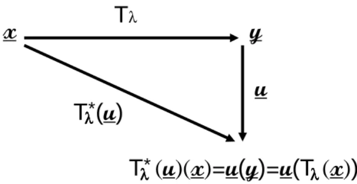
Obviously, G = I d (I d being the identity matrix) corre-sponds to the classical, scalar scaling (Eq. 18). It is now con-venient to use the notion of a “pullback” transform (or “com-position operator”, Shapiro, 1993) of a field u by a given space transform, here a contraction/dilation Tλ. It is so
gen-eral that it is often passed over without mention and it can be just seen as a convenient and compact notation for the scaling of a given field. As illustrated by Fig. 2, the pullback T∗
λ
cor-responds to a straightforward generalisation to (infinite di-mensional) functional spaces of the (contravariant) change of coordinates on (finite dimensional) vector spaces:
∀x : Tλ∗(u)(x) = u(Tλx) (21)
The composed function u(Tλ) pulls back the field u from
the coordinates y to x, with the “change of coordinates”
y = Tλ(x) (for further discussion see Schertzer et al., 2010;
Schertzer and Lovejoy, 2011). This transform can be ex-tended for differential operators D:
∀f : Tλ∗(D)Tλ∗(f ) = Tλ∗(Df ) (22)
For instance, the pullback of the gradient operator ∇ is:
Tλ∗(∇) = Tλ−1∇ (23) due to the fact that the transform Tλis linear and is therefore
its own Jacobian matrix. To study the (possible) anisotropy of atmospheric dynamics, it is sufficient to consider a diago-nal generator under the following form:
G = diag(gi); g1=g2=1; g3=Hz=1 − h (24)
T
λT ( )
*
T
( )( )
( )
(T
( )
)
λλλλ λλλλ*
λλλλFig. 2. Scheme of the “pullback” Tλ∗that pulls back the field u from the coordinates y to x with the help of the (anisotropic) space contraction/dilation Tλ.
with an exponent 0 ≤ Hz≤1 that defines the anisotropy of
Tλ. For instance, Hz=0 corresponds to a (scaling) 2-D flow,
Hz=1 to a 3-D (isotropic scaling) flow, and more generally
intermediate values to a (2+Hz) – dimensional (anisotropic)
scaling flow. Now, a generalised scaling of the field u(x,t ) is defined by the fact that its pullback transform Tλ∗ corre-sponds to a (possibly random) generalised contraction with a generator Ŵ:
Tλ∗u = λŴu (25)
The simplest case corresponds to the fact that both generators
G and Ŵ commute, i.e. are diagonal on the same vector base.
We consider the following particular case:
Ŵ = diag(γi); γ1=γ2=γ ; γ3=γ + h (26)
where γ is a given (scalar) singularity.
To give an illustration, let us consider the scaling model of a stratified atmosphere based on the conservation (i.e. strict scale invariance) of the energy flux along the horizon-tal and of the buoyancy force variance flux along the ver-tical (Schertzer and Lovejoy, 1984, 1985b). These conser-vation laws single out respectively the Kolmogorov’s sin-gularity γK= −1/3 and the Bolgiano-Obukhov singularity
γBO= −3/5. The latter is obtained similarly to the
for-mer, but for a flux that scales like u3/ l5 (Bolgiano, 1959; Obukhov, 1962). Note that these scaling exponents were both obtained assuming homogeneous and isotropic fluxes, whereas Schertzer and Lovejoy considered heterogeneous and anisotropic fluxes. In this anisotropic framework the the-oretical value Hz=5/9 of the exponent of anisotropy merely
results from the correspondence between the singularities of Kolmogorov and Bolgiano-Obukhov: γK=Hz·γBO.
The choice of having the same h in Eqs. (24), (26) not only makes, regardless of the h value, the incompressibility condition scale invariant, but also ensures that the advection term and the material derivative have the same scalar scaling:
D. Schertzer et al.: Quasi-geostrophic turbulence and generalized scale invariance 333
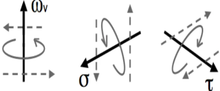
Fig. 3. Scheme of the vertical vorticity ωv, generated by the
hori-zontal shears of the horihori-zontal velocity, and the two components of the horizontal vorticity σ and τ generated respectively by horizontal shears of the vertical velocity and vertical shears of the horizontal velocity.
Because we consider an asymmetry between the horizon-tal and the vertical, it is useful both for the derivation and the expression of the fractional vorticity equations to decompose the fields and operators into horizontal and vertical compo-nents (with respective indices h and v), e.g. for the velocity field u and gradient operator ∇:
u = uh+uv;∇ = ∇h+∇v (28)
rather than with respect to a three-dimensional basis (e1,e2,e3), e.g.:
u = (u1,u2,u3); ∇ = (∂1,∂2,∂3); (29)
One readily obtains the following scaling for the velocity field u and gradient operator ∇:
Tλ∗(u) = λγ(uh+λhuv); Tλ∗(∇) = λ(∇h+λ−h∇v) (30)
Due to their difference of scaling (as confirmed below), we have to distinguish the horizontal vorticity components respectively yielded from vertical motions (σ ) and from hor-izontal motions (τ ), see Fig. 3 for illustration:
ω = ωv+ωh; ωh=σ + τ ; ωv≡∇h×uh; σ ≡ ∇h×uv; τ
≡∇v×uh (31)
It is straightforward to obtain the respective scaling of the vorticity components from Eqs.(30–31):
Tλ∗(ωv) = λ1+γωv;Tλ∗(σ ) = λ1+γ +hσ ; T ∗
λ(τ ) = λ1+γ −hτ (32) On the other hand, the stretching vector has the following decomposition:
s = ((σ + τ ) · ∇h+ωv·∇v)(uh+uv) (33)
that yields the following scaling ((σ · ∇h)uv=0 due to the
asymmetry of σ ):
Tλ∗(s) = λ2(1+γ )[ λh(σ · ∇h)uh+λ−h( τ · ∇h
+ωv·∇v)(uh+λhuv) ] (34)
Due to the fact that the vorticity equations should be sat-isfied for any λ, which appears with three distinct exponents (2(1+γ )(h,0,−h)), we obtain from Eqs.(27), (34) (ignoring for the present time the baroclinic vector) the following set of (barotropic) fractional vorticity equations:
Dσ /Dt = (σ · ∇h)uh (35)
Dτ /Dt = (τ · ∇h+ωv·∇v)uh (36)
Dωv/Dt = (τ · ∇h+ωv·∇v)uv (37)
which can be rewritten under the following coordinate form:
D∂2u3/Dt = (∂2u3∂1−∂1u3∂2)u1; −D∂1u3/Dt =(∂2u3∂1−∂1u3∂2)u2 (38) −D∂3u2/Dt = (∂1u2∂3−∂3u2∂1)u1;D∂3u1/Dt =(∂3u1∂2−∂2u1∂3)u2 (39) D(∂1u2−∂2u1)/Dt = ( ∂1u2∂3−∂3u2∂1+∂3u3∂2u3 −∂2u1∂3)u3 (40)
These equations (either under the vector or coordinate form) correspond to splitting the dynamical equation of the horizontal vorticity ωhinto two separate equations,
respec-tively for σ (the horizontal vorticity produced by vertical mo-tions) and τ (the horizontal vorticity produced by horizontal motions): this corresponds to the statistical break discussed above of the rotational symmetry of the original 3-D vortic-ity equations. Reciprocally, the latter equations are obtained by coupling again these equations, either under vector form (with (σ · ∇h)uv=0 as mentioned earlier):
D(σ + τ )/Dt = (σ + τ ) · ∇huh+ωv·∇vuh (41)
Dωv/Dt = (τ · ∇h+ωv·∇v)uv (42)
or under the coordinate form:
D(∂2u3−∂3u2)/Dt = ∂2u3∂1u1−∂1u3∂2u1+∂1u2∂3u1 −∂3u2∂1u1 (43) D(∂3u1−∂1u3)/Dt = ∂3u1∂2u2−∂2u1∂3u2+∂2u3∂1u2 −∂1u3∂2u2 (44) D(∂1u2−∂2u1)/Dt = ∂1u2∂3u3−∂3u2∂1u1+∂3u1∂2u3 −∂2u1∂3u3 (45)
This confirms the fact that solutions of Eqs. (35–37) form the subset of solutions of Eqs. (43–45) that statistically re-spect the anisotropic scaling prescribed by Eqs. (24), (26) and statistically break therefore the isotropic scaling of Eqs. (43–45).
Whereas the QG linearisation of the stretching vector keeps only the evolution of the vertical vorticity (Eq. 37), with a unique source term (ωv·∇v)uv and with the
fur-ther approximation ωv≃2, the fractional vorticity
equa-tions preserve all the nonlinearities. For instance, the term
(ωv·∇v)uh(in Eq. 36) tilts part of the vertical vorticity ωv
into the horizontal component τ , i.e. the latter does not nec-essarily remain zero if it was thus initially. The absence of a corresponding tilting term in the evolution equation of
σ (Eq. 35) shows that σ and τ have no symmetrical roles
and it also emphasises the importance of the splitting of the dynamical equation of horizontal vorticity into two separate equations. However, both σ and τ can undergo nonlinear stretching by (non-zero) horizontal gradients of the horizon-tal velocity (Eqs. 35–36), this implies in particular that so-lutions with σ = 0 are unstable. These features are illustra-tive of the huge difference between scale analysis and scal-ing analysis: in the former case (QG) all the source terms but one were cancelled in the vorticity equations, whereas in the present anisotropic scaling analysis, they are all pre-served but no longer contribute in an isotropic manner. For instance, the interactions of σ and τ with the horizontal gra-dient of the horizontal velocity become differentiated (with separate equations Eqs. 35–36), whereas only their sum in-tervenes in the 3-D vorticity equations (Eq. 41).
Although our paper is focused on the barotropic case, let us quickly show that the baroclinicity can be readily taken into account at all scales. Indeed, the baroclinic vector b has the following pullback:
Tλ∗(b) = λ2(γ +1)(λ−hbh+bv) (46)
One may note it has an opposite behaviour to that of the po-tential vector ψ :
Tλ∗(ψ ) = λγ −1(λhψh+ψv) (47)
which corresponds to the expected phenomenology: to be aligned along the vertical for large scales, whereas it is no longer the case for smaller scales. The comparison of the scaling of the vorticity components (Eq. 32) and of the baro-clinic vector (Eq. 46) shows that barobaro-clinicity does not affect the horizontal vorticity generated by vertical motions of σ , a fact that emphasises its particularity with respect to τ and
ωv. The barotropic fractional vorticity equations (Eqs. 35–
37) yield therefore the corresponding baroclinic equations:
Dσ /Dt = (σ · ∇h)uh (48)
Dτ /Dt = (τ · ∇h+ωv·∇v)uh+bh (49)
Dωv/Dt = (τ · ∇h+ωv·∇v)uv+bv (50)
The fractional vorticity equations (either barotropic, Eqs. 35–37) or baroclinic (Eqs. 48–50) were derived from the usual vorticity equations with the assumption of a given
anisotropic scaling behaviour (Eqs. 24–26) of particular so-lutions. An inspection of these derived equations shows that conversely their solutions should statistically respect this type of anisotropy, however there is no hint that the theoret-ical value Hz=5/9 plays a special role. Indeed, this
theo-retical value was obtained in fact with the help of thermo-dynamic considerations, whereas we explained that we post-pone to future works the treatment of the energy evolution equation in a similar manner to the way we treated the vor-ticity equations. On the other hand, it is worthwhile noting that the obtained fractional vorticity equations already corre-spond to an achievement that goes well beyond the question of the atmospheric dynamics scaling. Indeed, a precise def-inition of d-dimensional turbulence for non integer d’s has only been addressed in an isotropic and statistical framework (Fournier and Frisch, 1978) for the (average) energy spec-trum and with the help of a second-order closure, whereas we obtained (apparently) deterministic, dynamical equations for the field itself of the vorticity, and therefore of the veloc-ity. Furthermore, the fractional part Hz of this non integer
dimension is physically meaningful: Hzmeasures the extent
of the vertical motions, in fact the fractional depth of the cor-responding pancake turbulence, from 0 (flat 2-D turbulence) to 1 (3-D turbulence).
5 Conclusions
We believe that the critical analyses of the scale analysis leading to the QG approximation (Sect. 2) and of the scal-ing analysis of the resultscal-ing QGT (Sect. 3) first rule out LT-NCG’s claim that the significance of the spectrum power law
E(k) ≈ k−3 on scales ≥ 600 km obtained from the GASP
and Mozaic databases could not be brought into question be-cause it corresponds to a QGT prediction. Beyond this neces-sary clarification, we furthermore put forward an alternative (Sect. 4) to the QG approximation that reconciles the facts that Earth’s rotation dominates vorticity at large scales and that the vorticity stretching nonlinearly transfers this large scale input over a wide range of scales in a scaling man-ner. Indeed, by introducing a statistical anisotropic break of the statistical isotropic scaling of the vorticity equations, we obtain fractional vorticity equations, whose solutions should statistically satisfy this anisotropic scaling over a wide range of scales and therefore define a turbulence of (fractal) dimen-sion D = 2 + Hz(0 ≤ Hz≤1). This corresponds to the
dy-namical step towards this alternative to QG, which should be completed by a similar treatment of the thermodynamic en-ergy evolution equation. Overall, our claim that atmospheric turbulence has a dimension D = 2+Hz, presumably with the
theoretical value Hz=5/9, and is therefore so much distinct
from quasi-2-D and quasi-3-D turbulences, seems to result from the application of “Occam’s Razor” in the framework of a fruitful dialogue between theories and data, as defined by Medawar (1969): “scientific reasoning is a kind of dialogue
D. Schertzer et al.: Quasi-geostrophic turbulence and generalized scale invariance 335
between the possible and the actual, between what might be and what is in fact the case”.
Acknowledgements. We thank the editor and both anonymous
referees for their comments and suggestions that greatly helped us to improve our manuscript. D. Schertzer acknowledges stimulating discussions with J. P. Chancelier and A. Ern on the obtained fractional vorticity equations. We thank A. Krzykowski for her help to solve unexpected typesetting problems.
Edited by: G. Vaughan
References
Adelfang, S. I.: On the relation between wind shears over various intervals, J. Atmos. Sci., 10, 156–159, 1971.
Bourgeois, A. J. and Beale, J. T.: Validity of the quasigeostrophic model for large-scale flow in the atmosphere and ocean SIAM, J. Math. Anal., 25, 1023–1068, 1994.
Billant, P.: Zigzag instability of vortex pairs in stratified and rotating fluids. part 1. general stability equations, J. Fluid Mech., 660, 345–395, 2010.
Billant, P., Deloncle, A., Chomaz, J. M., and Otheguy, P.: Zigzag instability of vortex pairs in stratified and rotating fluids. part 2. analytical and numerical analyses, J. Fluid Mech., 660, 396–429, 2010.
Bolgiano, R.: Turbulent spectra in a stably stratified atmosphere, J. Geophys. Res., 64, 2226–2229, 1959.
Charney, J. G.: On the scale of atmospheric motions, Geophys. Publ. Oslo, 17, 1–17, 1948.
Charney, J. G.: Geostrophic Turbulence, J. Atmos. Sci., 28, 1087– 1095, 1971.
Charney, J. G., Fjortoft, R., and von Neumann, J.: Numerical inte-gration of the barotropic vorticity equation, Tellus, 2, 237–254, 1950.
Endlich, R. M., Singleton, R. C., and Kaufman, J. W.: Spectral Analyes of detailed vertical wind profiles, J. Atmos. Sci., 26, 1030–1041, 1969.
Ertel, H.: Ein neuer hydrodynamischer Wirbelsatz, Meteorol. Z., 59, 271–281, 1942.
Fjortoft, R.: On the changes in the spectral distribution of kinetic energy in two dimensional, nondivergent flow, Tellus, 7, 168– 176, 1953.
Forster, D., Nelson, D. R., and Stephen, M. J.: Large distance and long time properties of a randomly stirred fluid, Phys. Rev. A, 16, 732–749, 1977.
Fournier, J. D. and Frisch, U.: Remarks on renormalization group in statistical fluid dynamics, Phys. Rev. A, 28, 1000–1002, 1983. Fournier, J. D. and Frisch, U.: d-dimensional turbulence, Phys. Rev.
A, 17, 747–762, 1978.
Fu, L. L. and Flierl, G. R.: Nonlinear energy and enstrophy transfers in a realistically stratified ocean, Dyn. Atm. Oceans, 4, 219–246, 1978.
Gage, K. S.: Evidence for k-5/3 law inertial range in meso-scale two dimensional turbulence, J. Atmos. Sci., 36, 1950–1954, 1979. Goldstein, S.: Modern developments in Fluid Mechanics, Oxford
Univ. Press., Oxford, 1938.
Herring, J. R.: Statistical theory of quasi-geostrophic turbulence, J. Atmos. Sci., 37, 969–977, 1980.
Herring, J. R.: Turbulence, 69–76, McGraw-Hill, 2001.
Hua, B. L. and Haidvogel, B.: Numerical Simulations of the vertical structure of Quasi-Geostrophic Turbulence, J. Atmos. Sci., 43, 2923–2936, 1986.
Kolmogorov, A. N.: Local structure of turbulence in an incompress-ible liquid for very large Reynolds numbers, Proc. Acad. Sci. URSS., Geochem. Sect., 30, 299–303, 1941.
Kraichnan, R. H.: Inertial ranges in two-dimensional turbulence, Phys. Fluids, 10, 1417–1423, 1967.
Kraichnan, R. H.: Inertial-Range Transfer in Two- and Three-Dimensional Turbulence, J. Fluid Mech., 47, 513–525, 1971. Lesieur, M.: Turbulence in Fluids, 4th edition, Springer, Dordrecht,
2008.
Lesieur, M. and Schertzer, D.: Amortissement auto-similaire d’une turbulence `a grand nombre de Reynolds, J. Mec., 17, 249–280, 1978.
Lilly, D. and Paterson, E. L.: Aircraft measurements of atmospheric kinetic energy spectra, Tellus, 35A, 379–382, 1983.
Lindborg, E.: Can the atmospheric kinetic energy spectrum be ex-plained by two-dimensional turbulence?, J. Fluid Mech., 388, 259–288, 1999.
Lindborg, E., Tung, K. K., Nastrom, G. D., Cho, J. Y. N., and Gage, K. S.: Comment on “Reinterpreting aircraft measurement in anisotropic scaling turbulence” by Lovejoy et al. (2009), At-mos. Chem. Phys., 10, 1401–1402, doi:10.5194/acp-10-1401-2010, 2010.
Lovejoy, S., Tuck, A. F., Schertzer, D., and Hovde, S. J.: Reinter-preting aircraft measurements in anisotropic scaling turbulence, Atmos. Chem. Phys., 9, 5007–5025, doi:10.5194/acp-9-5007-2009, 2009a.
Lovejoy, S., Tuck, A. F., and Schertzer, D.: Interactive com-ment on “Comcom-ment on “Reinterpreting aircraft measurecom-ments in anisotropic scaling turbulence” by Lovejoy et al. (2009)” by E. Lindborg et al., Atmos. Chem. Phys. Discuss., 9, C7688– C7696, 2009b.
McWilliams, J. C., Weiss, J. B., and Yavneh, I.: Anisotropy and coherent vortex structures in planetary turbulence, Science, 264, 410–413, 1994.
Medawar, P. B.: Induction and intuition in scientific thought, Amer-ican Philosophical Society, Philadelphia, 1969.
Monin, A. S.: Weather forecasting as a problem in physics, MIT Press, Boston MA, 1972.
Mueller, P..: Ertel’s potential vorticity theorem in physical oceanog-raphy, Rev. Geophys., 33, 67–97, 1995.
Obukhov, A. M.: Some specific features of atmospheric turbulence, J. Fluid. Mech., 13, 77–81, 1962.
Pedlosky, J.: Geophysical Fluid Dynamics, Springer-Verlag, Berlin, Heidelberg, New-York, 1979.
Robinson, G. D.: Some current projects for global meteorological observation and experiment, Q. J. Roy. Meteor. Soc., 93, 409– 418, 1967.
Salmon, R.: Two-layer quasi-geostrophic turbulence in a simple special case, Geophys. Astrophys. Fluid Dynamics, 10, 25–52, 1978.
Salmon, R., Holloway, G., and Hendershott, M. C.: The equilib-rium statistical mechanics of simple quasi-geostrophic models, J. Fluid Mech., 75, 691–703, 1978.
Schertzer, D. and Lovejoy, S.: On the Dimension of Atmospheric Motions, 505–512, Elsevier, Amsterdam, 1984.
Schertzer, D. and Lovejoy, S.: The dimension and intermittency of atmospheric dynamics, 7–33, Springer-Verlag, 1985a.
Schertzer, D. and Lovejoy, S.: Generalised scale invariance in tur-bulent phenomena, Physico-Chemical Hydrodynamics Journal, 6, 623–635, 1985b.
Schertzer, D. and Lovejoy, S.: Space-time Complexity and Multi-fractal Predictability, Physica A, 338, 173–186, 2004.
Schertzer, D. and Lovejoy, S.: Mulitfractals, generalized scale in-variance and complexity in geophysics, International Journal of Bifurcation and Chaos, 21, 1–41, 2011.
Schertzer, D., Tchiguirinskaia, I., Lovejoy, S., and Hubert, P.: No monsters, no miracles: in nonlinear sciences hydrology is not an outlier!, Hydrol. Sci. J., 55, 965–979, 2010.
Shapiro, J. H.: Composition operators and classical function theory, Springer-Verlag, New York, 1993.
Smith, K. S.: Comment on: “The k-3 and k-5/3 energy spectrum of atmospheric turbulence: Quasigeostrophic two-level model sim-ulation”, J. Atmos. Sci., 61, 937–941, 2003.
Tung, K. K. and Orlando, W. W.: The k−3 and k−5/3 energy spectrum of atmospheric turbulence: Quasigeostrophic two-level model simulation, J. Atmos. Sci., 60, 824–835, 2003.
Vallis, G. K.: On the spectral integration of the quasi-geostrophic equations for doubly-periodic and channel flow, J. Atmos. Sci., 42, 95–99, 1985.
Van der Hoven, I.: Power spectrum of horizontal wind speed in the frequency range from.0007 to 900 cycles per hour, J. Meteorol., 14, 160–164, 1957.
Welch, W. T. and Tung, K. K.: Nonlinear baroclinic adjustment and wave-number selection in a simple case, J. Atmos. Sci., 55, 1285–1302, 1998.
Yano, J.-I.: Interactive comment on “Why anisotropic turbulence matters: another reply” by S. Lovejoy et al., Atmos. Chem. Phys. Discuss., 10, C1625–C1629, 2010.
Yano, J.-I.: Interactive comment on “Quasi-geostrophic turbu-lence and generalized scale invariance, a theoretical reply” by D. Schertzer et al., Atmos. Chem. Phys. Discuss., 11, C1213– C1215, 2011.