Drying of colloidal suspension drops : pattern formation and mechanical deformation

(1)

Drying of colloidal suspension drops:

pattern formation and mechanical deformation

by

Paul Lilin

Titre d’Ingénieur, École polytechnique (2018)

Submitted to the Department of Mechanical Engineering

in partial fulfillment of the requirements for the degree of

Master of Science in Mechanical Engineering

at the

MASSACHUSETTS INSTITUTE OF TECHNOLOGY

May 2020

c

○ Massachusetts Institute of Technology 2020. All rights reserved.

Author . . . .

Department of Mechanical Engineering

May 15, 2020

Certified by . . . .

Irmgard Bischofberger

Assistant Professor

Thesis Advisor

Accepted by . . . .

Nicolas Hadjiconstantinou

Chairman, Department Committee on Graduate Theses

(2)

(3)

Drying of colloidal suspension drops:

pattern formation and mechanical deformation

by

Paul Lilin

Submitted to the Department of Mechanical Engineering on May 15, 2020, in partial fulfillment of the

requirements for the degree of

Master of Science in Mechanical Engineering

Abstract

The drying of drops of colloidal suspensions on a hydrophilic substrate leads to the formation of a close-packed solid particle deposit. The initial volume fraction of particles sets the shape and size of this deposit, from a ring at the edge of the drop to a solid film covering the initial wetted area. We show that this deposit remains saturated with water and we explain the propagation of the solidification front by considering the evaporative flux and mass conservation. As the deposit forms, tensile drying stresses generate regularly spaced radial cracks. The crack patterns define four different regimes which we relate to experimental measurements of the deposit shape. The radial cracks separate the deposit into a multitude of petals. Due to the negative water pressure inside the pores of the deposit, these petals bend upwards creating mesmerizing forms reminiscent of blooming flowers.

Thesis Advisor: Irmgard Bischofberger Title: Assistant Professor

(4)

(5)

Acknowledgments

I would like to express my gratitude to Irmgard Bischofberger for her guidance and her unrelented enthusiasm. Thank you Irmgard for always being here for your students and for supporting me through the writing of this thesis.

I also thank Philippe Bourrianne, who was crucial in getting me established at MIT and in the lab. Philippe contributed greatly to this project, both from his own work and by coaching and coordinating multiple generations of visiting students. Thank you Philippe for teaching me sleek design presentation and for our endless bilingual discussions.

I had the chance to work with Guillaume Sintes, a visiting student who conducted or started some of the experiments in this thesis and made being in lab more fun. Watch out Guillaume, the microscope camera recorded some of your singing. I hope we can share time in the mountains soon!

I would also like to thank all the group members and visiting students: Jae Hyung Cho, Qing Zhang, Sami Yamanidouzisorkhabi, Ippolyti Dellatolas, Ashraf Kasmi, Andrew Griese, Traian Nirca, Alice Pelosse, and many other visiting students who have made and make HML a lively space, along with the rest of HML members and staff. A special thank you to Bavand Keshavarz and Michela Geri, whose warmth and hospitality brings everyone together.

Even though MIT can take over our lives at times, living in a new country is not all about research. I thank the MIT Climbing Team, and all my friends in Cambridge and beyond. They make me grow... and drive me to the mountains every week-end for some adventures! Thank you Nicolas, Kathy and the rest of MITOC for showing me that lack of sleep does not matter when you are having so much fun! #blessed

Finally, I thank my parents, who are always kind and supportive and to whom I owe more than I can write.

(6)

(7)

List of Figures

1-1 Crack patterns for different initial particle volume fractions . . . 20

1-2 Photographs of a drop drying in the single-crack regime . . . 22

2-1 Deposition of a drop of Ludox suspension . . . 26

2-2 Temporal evolution of the mass and drying rate evolution for drops of water and Ludox suspension . . . 28

2-3 Estimated evaporative flux as a function of relative humidity . . . 31

2-4 Normalized drying rate versus calculated volume fraction . . . 33

2-5 Expression to find the evaporative flux and the deposit volume fraction from the total drying time . . . 35

3-1 Scanning Electron Microscope image of the deposit . . . 38

3-2 Sketch of deposit initiation and growth . . . 39

3-3 Laser confocal profilometer structure and confocal principle . . . 42

3-4 Profile measurement during drying . . . 44

3-5 Profile measurement after drying . . . 46

3-6 Final moments of drying for a drop in the coffee-ring regime . . . 47

3-7 Ring-crack and double-crack deposit profiles . . . 48

3-8 Transition from coffee-rings to ring-cracks and double-cracks . . . 49

3-9 Single-crack deposit profiles . . . 50

3-10 Deposit height versus initial volume fraction . . . 51

3-11 Temporal evolution of the deposit volume . . . 55

3-12 Deposit volume growth . . . 56

(12)

4-1 Generation of tensile stresses in the deposit . . . 61

4-2 Definition of stresses in the deposit . . . 61

4-3 High speed interference microscopy images of the deposit at the mo-ment of the appearance of the first crack . . . 63

4-4 Definition of variables used to model to pressure in the deposit . . . . 66

4-5 Model for deposit width at onset of fracture . . . 67

4-6 The propagation of cracks . . . 68

4-7 Crack spacing for different drops in the single-crack regime . . . 68

4-8 High speed interference images of crack generation . . . 70

4-9 Propagation of a pair of cracks in a thin film . . . 71

4-10 Crack spacing versus deposit thickness . . . 72

4-11 Number of cracks and angular crack spacing versus initial volume fraction 73 4-12 Radial propagation of a crack in the single-crack regime . . . 74

4-13 Radial propagation of a crack in the double-crack regime . . . 75

4-14 Comparison between two forms of ring-crack . . . 77

5-1 Sketch of the deposit pore pressure variation in the vertical direction 80 5-2 Sketch of the proposed model for bending of the deposit . . . 84

5-3 Sketch of interferometry setup . . . 86

5-4 Analysis of interferometry data. . . 86

5-5 Petal bending profile at different times and parabolic fit . . . 88

5-6 Bending dynamics . . . 89

5-7 Curvature A versus normalized deposit width and petal shape at largest curvature . . . 89

5-8 Normalized maximal petal curvature versus initial volume fraction . . 90

5-9 Side-view measurement of the tip deflection 𝛿 . . . 92

5-10 Comparison between petal tip displacement predicted by interferome-try and measured value in side-view . . . 93

5-11 Photograph of drops shape after drying . . . 94

(13)

5-13 Discontinuous and continuous tip deflection dynamics depending on initial volume fraction . . . 96 5-14 Geometrical constraint at large scale bending for drops of low initial

volume fraction . . . 97 5-15 Undulations of the crack tip for larger initial radius . . . 98 6-1 Temporal evolution of a 2 µL drop of Ludox suspension on a

hydropho-bic substrate . . . 100 6-2 Buckling and air invasion in a 2 µL drop of initial volume fraction

𝜑0 = 0.23 on a hydrophobic substrate. . . 101

6-3 Example of directional drying. Two 0.3 µL drops with 𝜑0 = 0.08 are

deposited next to each other. . . 102 B-1 Definition of variables used in the model for pressure in the deposit . 108 B-2 Results of the pressure model. Dimensionless velocity, maximum

pres-sure and prespres-sure versus dimensionless radius and time . . . 111 C-1 Definition of the parameters used for bending . . . 114 C-2 Geometry for bending in the case of a linear profile . . . 114

(14)

(15)

Chapter 1 Introduction

Colloidal suspensions are ubiquitous in daily life, from coffee and milk to cosmetics and paints, and even blood [38]. Once dried, these colloidal systems form coatings that are prone to failure, as evidenced by the formation of craquelures in ancient paintings or in mud [30]. Similarly, droplets of colloidal suspensions leave a variety of solid deposit as they dry depending on the amount of suspended particles; from the well-known coffee-ring effect in dilute suspensions [7] to homogeneous coatings at larger colloid concentrations [11]. These deposits exhibit beautiful crack patterns and surprising mechanical deformations. In this work, we study the deposition dynamics, crack pattern and mechanical deformation that occur for small droplets as we vary the volume fraction of nanoparticles.

Despite its simple appearance and its small size, the drying of a concentrated colloidal drop is a very complex process. A multiplicity of patterns can appear [13] depending on the type of colloids, the size of the drop and the drying conditions. During drying, the flow in the drop and the interactions between the particles influence the formation of a solid deposit. The properties of this deposit can vary in space and with time as it consolidates. Air can penetrate inside this deposit, or it can delaminate or buckle, or it can shatter and send fragments flying. In this chapter we give a brief overview of the physics at play and we introduce the patterns that we observe.

(16)

1.1 Drying of sessile drops

What shape does a drop of water take when it is deposited on a flat dry substrate? Two effects are at play: surface tension efects, which tend to maintain a uniform curvature and thus a spherical cap shape; and gravity effects, which tends to flatten the drop. For drop sizes smaller than the capillary lengthscale 𝜅−1 ₌ _√︀𝛾

𝑤/(𝜌𝑤𝑔) =

2.71 mm, surface tension is dominant and the drop adopts the shape of a spherical cap. Here 𝛾𝑤is the water-air surface tension, 𝜌𝑤 the density of water and 𝑔 the gravitational

acceleration. The drop shape is then completely defined by two parameters, the contact radius 𝑅 and the contact angle 𝜃.

However, the drop does not retain its shape for long. It dries and loses volume until it disappears. Why? At the liquid-air interface, water molecules jump from one side to the other at a very high frequency [4]. The air surrounding the drop is thus saturated in water vapor. Far away from the drop, the concentration in water vapor is only a fraction of this saturated value. This proportion is the relative humidity (𝑅𝐻). As the water vapor molecules diffuse away from the liquid vicinity, more liquid water can evaporate and the liquid volume decreases. Water vapor diffusion is the rate-limiting process for evaporation in the absence of air flow (convective evaporation).

We define the evaporative flux 𝑉𝐸 as the volume of water that evaporates from

a surface per unit area and per unit time. 𝑉𝐸 has the dimension of a velocity: the

retraction velocity of the interface if there is no additional flow in the liquid. 𝑉𝐸 is

obtained by solving the diffusion equation 𝜕𝑐/𝜕𝑡 = ∆𝑐. Solving the three dimensional diffusion equation for a spherical shape is not an easy task. For small contact angles and slow variations in time, an electrostatic analogy with the capacitance of a con-ducting lens can be made [7]. However, this analogy neglects thermal effects which change the value of the evaporative flux.

The most important feature of the evaporative flux for sessile drops is that it is not uniform. In the case of hydrophilic surfaces, when the contact angle 𝜃 is lower than 90∘, the evaporative flux is higher at the edge of the drop. For 𝜃 = 90∘, the problem is symmetric and the evaporative flux is uniform, and for hydrophobic surfaces with

(17)

𝜃 > 90∘ the evaporative flux is greater at the apex of the drop. This variation can be understood from the diffusive nature of the problem. For a drop on an hydrophilic surface, a water vapor molecule next to the edge is surrounded by a less saturated atmosphere than if it were at the drop apex. It has more unsaturated directions to diffuse to, thus evaporation happens faster. This asymmetry of the evaporative flux can drive flows inside the liquid, as we will see in section 3.1.

An exhaustive review on the drying of sessile drops of pure liquids is found in [4].

1.2 Colloidal suspensions

While there remain some discrepancies between analytical formulas and experimental measurements, the drying of pure liquids in well understood. However, the drops we are interested in are made of a colloidal suspension, and the drying of these systems still involves many open questions.

A colloidal suspension is a complex fluid comprised of a liquid (in our case, water) and solutes smaller than the colloidal limit, but larger than liquid molecules: 1 nm < 𝑎 < 500 nm [5]. Due to the small size of the particles, thermal agitation dominates gravitational effects and the particles do not sediment.

In addition to thermal fluctuations, there is a balance between attraction and repulsion between the particles. The attraction force is the van der Waals force [32], caused by an interaction between the fluctuating electromagnetic fields associated with the particles polarizabilities. In the cases we are interested in, the repulsion force is the electrostatic double-layer force [32]. The colloids we are interested in are negatively charged; they attract positive ions and the charges surrounding each particle repel each other. The combination of these two forces constitutes the DLVO theory of colloidal suspension stability. In our case, all the base suspensions are stable. A colloidal suspension can become unstable following a change in temperature or in ion concentration. This means that the attractive force overcomes the repulsion, and the suspension forms a gel. For a bulk fluid, the transition from a stable suspension to a gel is slow, it typically takes from ten minutes to a few hours.

(18)

1.3 Drying of colloidal suspensions

Colloidal suspensions are usually studied in the bulk, where the concentration can be assumed to be uniform. This is no longer true when a colloidal suspension is drying. This makes the drying of colloidal suspension a complex problem. We will summarize some of the key processes.

The increase in volume fraction 𝜑 in the suspension can be described by a non-linear advection-diffusion equation where the diffusion coefficient depends on 𝜑. The non-linearity comes from the large volume fraction of particles as liquid is removed. Even then, this equation can only be used below a critical volume fraction. When the volume fraction reaches a critical value, the viscosity diverges and the suspension essentially behaves as a solid. We call this solidified suspension a deposit; a porous material that can be described by the poroelasticity theory [47]. Because of the small size of the pores between the particles, capillary forces prevent air from penetrating inside the deposit until the pressure difference is strong enough.

The particles are not simply packed together; interparticle attractive forces (eg van der Waals forces) hold the deposit together such that re-introducing water does not re-disperse it. For polymer colloidal suspensions (latex), the particles can coalesce into a film and fill essentially all the voids before air penetrates inside the deposit. For hard particles such as silica nanoparticles, the particle volume fraction is limited to an absolute maximum of 74 % (ordered close packing). Air invades the deposit after the particles have consolidated. These different scenarios for particle deformation, film formation and air invasion have been rationalized depending on the particle size and mechanical properties [39].

Regarding the dynamics of drying, there are two limiting cases, sometimes called horizontal and vertical drying [13][38].

1.3.1 Vertical drying

Vertical drying is what happens in an open jar full of a colloidal suspension. The thickness 𝐻 (length normal to the drying surface) is much larger than the width

(19)

of the area exposed to drying. For 𝑃 𝑒𝑉 = 𝑉𝐸𝐻/𝐷 ≫ 1, advection dominates and

particle diffusion is too slow to smooth the concentration profile. A concentrated skin is formed that dominates the mechanical deformation. This situation arises for drops of high particle volume fraction on a hydrophobic surface [2]. For drops on hydrophilic surfaces, this effect is negligible.

1.3.2 Horizontal drying

Horizontal drying is related to the drying of thin films. It is characterized by a large free surface exposed to air 𝐿2, with 𝐿 much larger than the film thickness 𝐻. The

vertical Péclet number 𝑃 𝑒𝑉 is then taken to be zero. In the case of sessile drops

on hydrophilic surfaces, the evaporative flux is greater at the edge. Because of this directionality, the edges are the first to undergo a liquid to solid transition and to form a deposit: a solidification front propagates across the film. Such films often form cracks, and these cracks propagate in the same direction. These fronts are crucial in our experiments.

1.4 Pattern formation in drops

One of the most ubiquitous patterns formed by drying colloidal suspension drops is the coffee-ring effect [7]. This pattern appears for suspensions of particles at low vol-ume fraction on hydrophilic surfaces. The particles accumulate at the drop edge. In the case of coffee, this accumulation results in the familiar coffee stains. A large body of literature explores how to suppress and tune this pattern [1], which is achieved by tuning either the flow (eg Marangoni flows), the particle-particle interactions (eg rod-shaped particles) or the particle interactions with the solid-liquid and liquid-air boundaries (eg surfactants). A number of deposition patterns are obtained this way, including deposition in the center dubbed "coffee eye" [24] or uniform cover-age. However, these patterns at low particle volume fraction remain essentially two dimensional, with a thickness of a few particles.

(20)

flow, its adhesion with the substrate and its mechanical properties determine the pattern. For drops, studies have probed the importance of gelation [35], particle deformability [46] and relative humidity [11]. However, most of the studies are con-cerned with either films or constrained geometries similar to Hele-Shaw cells where the drying only occurs at the edge. These geometries are easier to control. However, using drops produces more striking patterns, including surprisingly large mechanical deformations.

At the other limit of the volume fraction range, latex coatings have also been studied extensively [38]. The interest in these films comes from the industries needs to obtain crack-free coatings.

1.5 Overview: blooming flowers

(a) Coffee ring 𝜑0 = 4 × 10−4 (b) Ring-crack 𝜑0 = 8 × 10−3 (c) Double-crack 𝜑0= 0.018 (d) Single-crack 𝜑0 = 0.21

Figure 1-1: Crack patterns for different initial particle volume fractions 𝜑0.

Our study bridges the two extremes as we increase the initial particle volume fraction of a suspension of silica nanoparticles from 10−4 _{to 0.23. We keep a constant}

particle size and chemistry so that the deposit maintains the same properties. Figure 1-1 gives an overview of the four different regimes we observe with increasing initial volume fraction, identified by their crack pattern:

(21)

(a) the coffee-ring regime, where no cracks are visible and the deposit width is much smaller than the drop radius;

(b) the ring-crack regime, where we first see radial cracks. The cracks only extend over a ring;

(c) the double-crack regime, where the radial cracks extend all the way to the center of the deposit. However the cracks branch at a well defined radius;

(d) the single-crack regime, where the radial cracks extend straight from the deposit edge to the center.

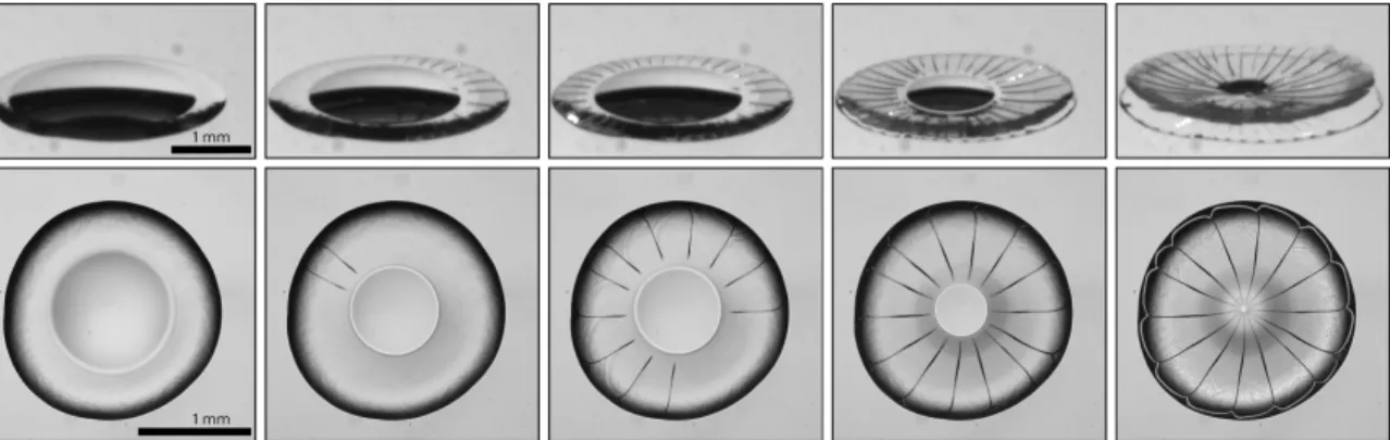
For all regimes except the coffee-ring, we observe a strikingly regular crack spacing. In addition to the crack pattern, we are interested in the dynamics of the deposit formation and in the mechanical deformation, particularly in the single-crack regime. These dynamics are shown in figure 1-2. We present images both from the side and from below. We observe several important features, which we explore in more details in the following chapters:

∙ the drop is characterized by two distinct features; a receding liquid cap in the center and a growing solid deposit around it. We study the dynamics of the deposit growth and liquid cap retraction in chapter 3.

∙ a crack forms at a certain deposit width, then more cracks appear with a constant spacing. We study these cracks in chapter 4.

∙ the cracks propagate towards the center, delimiting separate areas in the deposit that we call petals;

(22)

Figure 1-2: Photographs of a drop drying in the single-crack regime from the side (top) and from below (bottom). Two different drops of the same initial volume fraction 𝜑0 = 0.21 are used to compose the image. The elapsed time is 80 s, drops

(23)

Chapter 2 Evaporation process

Before we study the formation, cracking and bending of the deposit, we need to know more about our experimental conditions and about the properties of this deposit.

Evaporation If a drop of a colloidal suspension were deposited in an atmosphere fully saturated with water, it would sit still and nothing would happen. As the particle size is below the colloidal limit, there is no sedimentation. If the atmosphere is not saturated, water vapor diffuses away from the drop. This diffusion is the only cause for change in our experiments. It drives the formation of a particle deposit and generates the stresses that bend this deposit.

At the drop level, evaporation is characterized by the drying rate ˙𝑚 where 𝑚 is the mass of the drop. We can also define a mean evaporative flux 𝑉𝐸 such that

˙

𝑚 = 𝜌𝑆𝑉𝐸 with 𝑆 the surface area of the drop. Locally, the relevant variable is the

evaporative flux 𝑗 (in m s−1_{), the volume of water removed from the drop per meter}

square per second.

Deposit As the drop dries a solid deposit region appears. This deposit remains wet for the duration of the experiment and is comprised of close-packed nanoparticles and water. We assume that this deposit has a constant particle volume fraction, 𝜑𝑔.

(24)

2.1 Methods

2.1.1 Colloidal suspension

All the experiments are performed using aqueous suspensions of silica particles (Ludox AS-40) diluted with deionized water. The diameter of the particles is 20 - 22 nm. The suspension is stabilized by the addition of small amounts of alkali (ammonia) producing ammonium hydroxide anions. The hydroxyl ions react with surface silanol groups to create negative surface charges, which cause the particles to repel each other [31].

As the suspension dries, the effective salt concentration increases. This can screen the electrostatic repulsion and lead to gelation if the van der Waals forces overcome electrostatic repulsion [17]. This process is driven by kinetics of interparticle collisions and has an associated timescale 𝑡𝑔. Gelation can give rise to a variety of pattern if

the drying is slow enough [15]. However, measured values of 𝑡𝑔 [35] are much larger

than the drying time in our experiments.

Ludox AS40 has a reported mass fraction of 0.395 0.41 and a density of 1.286 -1.300 g cm−3. From these values the volume fraction can be estimated to be 0.227 (see appendix A for the derivation). In our experiments, the volume fraction is varied between 10−6 _{and 0.227 by adding deionized water.}

2.1.2 Substrate

We use glass microscope slides for the pattern formation experiments and small cov-erslips for the mass measurement experiments. We clean the glass by sonicating for 5- 20 minutes in acetone, then rinsing with acetone and isopropanol, and finally drying with compressed nitrogen or occasionally compressed air.

The advancing and receding contact angles for water are measured as 𝜃𝐴 =

(25)

2.1.3 Drop deposition

In preliminary experiments we observed that the pattern is independent of volume. We use small volume as the drop dries faster which allows us to perform more ex-periments. Another reason is that for drops of size smaller than the capillary length 𝜅−1 = √︀𝛾/(𝜌𝑔) = 2.71 mm, the effect of gravity is small compared to the effect of surface tension, and the shape of the initial drop is a spherical cap. Finally, small deposits are less prone to breakage when they beautifully bend upward. Most of the experiments are carried out using an initial volume of 0.3 µL.

In theory, depositing a drop on a surface can lead to any value of the contact angle between 𝜃𝐴 and 𝜃𝑅 depending how the drop is deposited. This uncertainty

is traditionally solved by changing the deposition method and removing the human factor. Perhaps the best method is to start dispensing the liquid, make it come into contact with the substrate, then finish dispensing the liquid, which reliably yields the advancing contact angle. Another method is to continuously pump the fluid into a needle and let the drop detach under the effect of gravity, keeping the falling height constant between experiments. However, in our case, two factors make it challenging to implement such methods:

1. The very small volume requires a precise system with no pressure loss, and it is not possible to use the first technique described above. One could use the needle technique but the diameter of the needle would have to be less than 200 µm for a volume of 1 µL.

2. The drop is composed of a suspension, which can dry out and become impossible to dispense. This is the main problem, which requires to pump the liquid in less than 20 - 30 s before deposition.

To overcome these challenges, we deposit the drops with a 0.2 - 2 µL precision pipette by hand, which does create some variability. However, the deposit contact angle is consistently found in the range 𝜃0 = (22 ± 2)∘, both for drops of Ludox and

(26)

Figure 2-1: Deposition of a drop of Ludox suspension. The time between each image is 0.2 s. The drop radius increases during a few tenths of a second as the initial flow settles, then remains pinned.

deposited volume Ω0. For drops of 1 2 µL the measured deposited volume is 0.1

-0.2µL lower than expected. Pre-wetting, pipetting immersion depth and deposition angle all become important at such small volumes [44].

In light of these findings, all calculations are made assuming a contact angle of 22∘.

2.1.4 Ambient conditions

Evaporation is affected by ambient conditions, namely temperature and relative hu-midity. Temperature is controlled in the laboratory, and variations in the absolute value of the temperature are small. We do not account for any variation due to temperature.

However, we have to account for changes in Relative Humidity (RH). First, RH varies strongly in the laboratory from one day to the next. Second, the drying rate depends linearly on RH, which makes controlling relative humidity critical in our experiments. Furthermore, we need to avoid convective drying due to air flow. We achieve this control by conducting the experiments in an air tight box. To reach the desired RH range inside, we place a small open container with either water, a silica drying gel, or a saturated salt solution in the box. The relative humidity is measured using a dedicated sensor [ref? Omega one, or arduino]. The box has a small latch that

(27)

we open for a few seconds at the start of each experiment to deposit the drop. This causes the RH to vary slightly and limits the precision to a few percents. This initial disturbance can also cause some spatial variability in RH, which we try to account for by placing the sensor carefully.

2.2 Mass measurements

Let us start our experimental results section with the simplest measurement one could think of: the mass of the drop as it dries. Conducting this classical experiment is, however, challenging for the very small masses of our drops: we need a scale precise to 10−3_mg_{. We use a Thermogravimetric Analyzer (Discovery TGA 1) at the}

Institute for Soldier Nanotechnologies (ISN), which has a 0.1 µg resolution. While the measurements are very precise, the instrument has two limitations for us: it takes about 80 s to initialize, and the drop is placed in an opaque furnace.

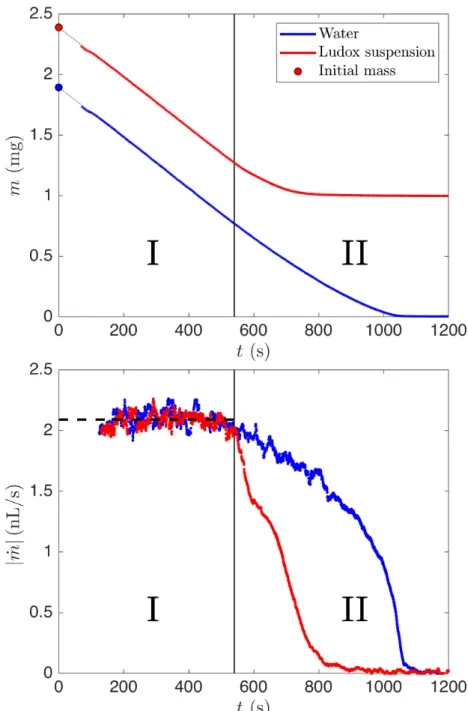
Because of the long initialization time, we increase the drop volume from 0.3 µL to 1 - 2 µL to increase the time it takes for the drop to evaporate. The measured evolution of the mass 𝑚 and total drying rate ˙𝑚 for water and a 0.23 volume fraction Ludox suspension are shown in figure 2-2.

Remarkably, the drying rate is initially constant and equal for a Ludox suspension and for water (region I). Why? The limiting process for evaporation here is the diffusion of water vapor in the surrounding air, which is the same for water or for a suspension [6].

Let us follow the temporal evolution of the drying rate of water. At first, the drying rate is constant, which is in agreement with the limiting process being the diffusion of water vapor and a constant surface area. However, at later times the drying rate decreases, which results from an unpinning of the water drop leading to a reduction in surface area.

For a Ludox suspension, we also observe a constant drying rate but the decrease is much sharper, defining region II. However, we see in figure 1-2 that the decrease of the liquid cap is smooth and cannot explain the decrease in drying rate. Actually,

(28)

Figure 2-2: Temporal evolution of the mass and drying rate evolution for drops of water and Ludox suspension, 𝜑0 = 0.23. The dotted lines in (a) indicate a linear fit,

which we use to calculate the initial mass. The dashed line in (b) indicate the reported initial drying rate, which is the same for Ludox suspension and water. In region I, the drying rate is constant. In region II, the drying rate of the Ludox suspension decreases abruptly.

(29)

the deposit remains wet throughout drying. Since the drying rate remains constant for a long time, the evaporative flux over the deposit must be the same as for pure water: diffusion is still the limiting factor. So what explains the sharp drop?

The drying rate decreases when the cost of pulling water out of the deposit be-comes too high. We will consider the pressure in more details in chapter 4. This pressure limit can be reached either because the deposit is very large, and thus water has to travel for a long distance, or because the reservoir of liquid water has disap-peared. The sharp decrease in ˙𝑚 points toward a well-defined transition time, so we expect the liquid cap disappearance to cause the drop in drying rate. The end of the liquid cap is followed a few seconds later by the end of mechanical deformations in the drop.

It follows that the drying rate remains constant over the time of mechan-ical deformation, and the evaporative flux is the same for the deposit and for the liquid.

Once the liquid cap has disappeared, evaporation of the water trapped in the deposit continues, but we soon reach a new regime where air invades the deposit. As silica and water have comparable refractive indices, but very different to the one of air, this air invasion is visible. However, it only occurs after all mechanical deformation has ended.

2.2.1 Estimate of evaporative flux 𝑉

𝐸

We aim to use the results from the mass measurements to estimate the evaporative flux and its dependence on the experimental parameters. Let us focus on the first region of figure 2-2 where the drying rate ˙𝑚 is constant.

While we know ˙𝑚, we do not have access to the surface area 𝑆 directly. We calculate the initial volume from the initial mass and the suspension density. Using the initial radius 𝑅0, and approximating for small 𝜃, the following equations hold true

(30)

for a spherical cap: Ω0 = 𝑔(𝜃)𝑅03 = 𝜋 3 (2 + cos(𝜃))(1 − cos(𝜃))2 sin3(𝜃) 𝑅 3 0 (︁ ≈ 𝜋 3𝜃𝑅 3 0 )︁ (2.1) 𝑆0 = 𝑓 (𝜃)𝑅20 = 2𝜋 1 − cos(𝜃) sin2(𝜃) 𝑅 2 0(︀≈ 𝜋𝑅20 )︀ (2.2) We see in equation 2.2 that the surface area depends on the contact angle, which varies with time. However the surface area is constant to the first order of 𝜃, so we will neglect its change. The mean evaporative flux 𝑉𝐸 = ˙𝑚/(𝜌𝑆) is thus constant in

region I.

Since we fix the value of the contact angle, we obtain 𝑉𝐸 = ˙ 𝑚 𝜌𝑆 = 𝑔2/3_(𝜃) 𝑓 (𝜃) ˙ 𝑚 𝜌Ω2/3₀ (2.3)

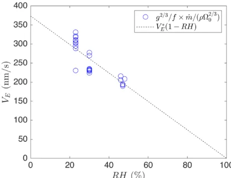
which we plot against RH in figure 2-3, with a dashed line showing the linear fit:

𝑉𝐸 = 𝑉𝐸*(1 − 𝑅𝐻) (2.4)

𝑉_𝐸* = (373 ± 15) nm s−1 (2.5)

Knowing the RH and the surface area, we can directly apply this equation to get the evaporative flux and drying rate of all experiments.

The diffusion problem for water vapor around a sessile drop of pure liquid has been shown to follow, for 𝜃 ≪ 1 [4]:

˙ 𝑚 = 𝜌2 𝜋𝐷𝑚 𝑛𝑠𝑎𝑡 𝑛𝑙 (1 − 𝑅𝐻)𝑅0 (2.6)

where 𝐷𝑚 is the coefficient of diffusion of water vapor in air, 𝑛𝑠𝑎𝑡 is the number

density of water molecule in the saturated air, and 𝑛𝑙 is the number density of water

molecule in water (liquid phase). For 𝑅0 = 900µm which we measure for drops of

initial volume Ω0 = 0.3µL this equation gives 𝑉𝐸* ≈ 780 nm s

−1_{. For drops of 1 - 2 µL}

the prediction is 𝑉*

𝐸 = 500 − 400 nm s −1_.

(31)

Figure 2-3: Estimated evaporative flux as a function of relative humidity for 20 drops of initial volume Ω0 = 0.75 − 2µL and initial volume fraction 𝜑0 = 0.09 − 0.23.

Evaporative flux 𝑉𝐸 is estimated according to equation 2.3.

of the drop. This stems from the dependence of the local drying flux as 𝑗 ∼ 𝑗0√ 1 𝑅20−𝑟2

which gives ˙𝑚 ∼ 𝑗0𝑅0. However, we found the "naive" scaling that assumes no

dependence of the mean evaporative flux on the radius to fit the data better. It would be interesting to perform experiments on larger drops to determine which scaling applies.

2.2.2 Estimate of deposit volume fraction 𝜑

𝑔

Now let us focus on the second region of figure 2-2. We make the hypothesis that the sharp decrease in drying rate is closely related to the disappearance of the liquid cap (figure 1-2). Without the liquid cap, all there is left is the deposit. We make another important hypothesis here: the deposit has a uniform volume fraction.

This hypothesis does not always hold true in the coffee-ring regime for very small initial volume fractions. In that case particles are initially deposited slowly and arrange in a crystal phase, while later particles are deposited faster and form an amorphous phase [27]. This shows that the deposit volume fraction can depend

(32)

slightly on the kinetics of deposition. However, in our experiments at higher volume fraction most of the deposit is created at a constant rate and we do not expect this effect to be important.

From these two hypotheses it appears that the volume fraction reached at the mo-ment the drying rate drops is the deposit volume fraction. From volume conservation of particles we can calculate the volume fraction as

𝜑 = 𝜑0 Ω0 Ω = 𝜑0 Ω0 Ω0− ∆𝑚/𝜌𝑤 (2.7) where 𝜌𝑤 is the density of water. As expected, 𝜑 increases with time. However,

once air penetrates the deposit equation 2.7 is no longer valid anymore as Ω = Ω0−

∆𝑚/𝜌𝑤+ Ω𝑎𝑖𝑟, and indeed it gives non-physical values of 𝜑.

The drying rate normalized by its initial value versus volume fraction is shown in figure 2-4. Since the deposition process is similar for drops of any volume fraction, we expect the deposit volume fraction to be the same for all drops. We make the following observations:

∙ the first sharp decrease in drying rate occurs at a volume fraction 𝜑1 ∈ [0.5, 0.6]

that increases with the initial volume fraction. It is not clearly defined for low initial volume fraction (lighter curves).

∙ all the curves rejoin at a volume fraction 𝜑2 ≈ 0.61. For high initial volume

fraction (darker curves) this corresponds to an inflection point in drying rate, which decreases more slowly before dipping again.

Without visual cues, it is hard to decide which value corresponds to the deposit volume fraction 𝜑𝑔. One potential scenario is that the first dip 𝜑1 occurs when the

outer part of the deposit reaches a critical pressure and evaporation locally slows down, although a liquid cap is still there. Only part of the deposit evaporates more slowly. Then the point where all the curves meet corresponds to the whole deposit evaporating at the same slow rate, and 𝜑2 would be the deposit volume fraction (if

(33)

Figure 2-4: Normalized drying rate versus volume fraction for 20 drops of initial volume Ω0 = 0.75 − 2µL at 𝑅𝐻 = 23 − 48 %. The volume fraction adopts unphysical

(34)

2.3 Total drying time

There is another measurement that is even simpler than measuring the mass: record-ing the time 𝑡𝑓 at which the drop is "fully dried". Obviously we need a more precise

definition, as we saw that evaporation continues for a long time after all mechanical deformation has ended. Let us define 𝑡𝑓 as the time when the liquid cap disappears.

2.3.1 Estimate of evaporative flux and deposit volume fraction

We found that the drying rate 𝑉𝐸𝑆 was constant over the time of interest. Making

the same hypothesis of uniform deposit volume fraction 𝜑𝑔, we can write conservation

equations for the volume of water and nanoparticles: 𝜑0Ω0 = 𝜑𝑔Ω𝑔 (1 − 𝜑0)Ω0− 𝑉𝐸𝑆𝑡𝑓 = (1 − 𝜑𝑔)Ω𝑔 which leads to 𝑡𝑓 = Ω0 𝑆𝑉𝐸 (︂ 1 −𝜑0 𝜑𝑔 )︂ (2.8) Using a microscope, we recorded 0.3 µL drops drying at different RHs.We observe a large spread in the radii of the deposited drops: 𝑅0 = (839 ± 114)µm. We attribute

this variability primarily to changes in the drop volume. Consequently we run into the opposite problem of section 2.2: while we know the (projected) surface area, the exact volume is unknown. We evaluate it by assuming the initial shape to be a spherical cap with a contact angle of 22∘_:

Ω0 =

𝑔(𝜃) 𝜋3/2𝑆

3/2 _(2.9)

where 𝑔(𝜃) was defined in equation 2.1.

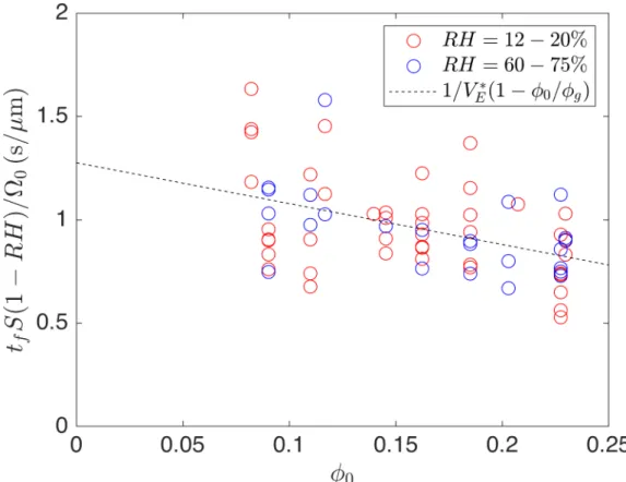
Using this approximation for the initial volume and equation 2.4 for the depen-dence of the evaporative flux on RH, we plot the following expression versus 𝜑0 in

(35)

Figure 2-5: Expression to find the evaporative flux and the deposit volume fraction from the total drying time. The expression is derived from equation 2.8 and the volume is estimated using equation 2.9.

figure 2-5: 𝑡𝑓 𝑆(1 − 𝑅𝐻) Ω0 = 1 𝑉* 𝐸 (︂ 1 −𝜑0 𝜑𝑔 )︂ (2.10) where we assume that the fitting parameters 𝑉*

𝐸 and 𝜑𝑔 are the same for all drops at

all RH. Although there is a large spread in the data, this rescaling works better than using the ˙𝑚 ∝ 𝑆/𝑅0 scaling found in the literature (equation 2.6). A linear regression

yields:

𝑉_𝐸* = (784 ± 50) nm s−1 (2.11)

𝜑𝑔 = 0.64 ± 0.16 (2.12)

It is interesting to note that the value of 𝜑𝑔 obtained does not depend on the

assumed contact angle, because we obtain it by dividing the intercept by the slope. However we note that this value has a large error estimate.

(36)

The disagreement between the value we obtain here of 𝑉*

𝐸 = (784 ± 50) nm s −1

and the value we obtained from mass measurement data 𝑉*

𝐸 = (373 ± 15) nm s −1

casts doubt on our assumption that the evaporative flux is independent of the drop radius, even though both data-sets individually support the hypothesis. To settle this issue, we plan to measure drying times for larger drops of the same contact angle.

In the following, we will use the value 𝑉*

𝐸 = (784 ± 50) nm s

−1 _{as a reference for}

(37)

Chapter 3 Formation of a particle deposit

In the previous chapter, we focused on the evaporation process, that is the removal of water. This transforms the drop material from a liquid to a solid deposit. We determined that this deposit had an average volume fraction in the range 50 - 64 % which is in accordance with values found in the literature for random close packing, depending on whether the particles are agitated or not [9].

The formation of this deposit is a fascinating process with complex underlying physics, as we saw in section 1.3. In this section, we will focus on the macroscopic mechanisms driving the deposit formation. We will report the main characteristics of the resulting deposit profile, which can influence mechanical deformation later on. At the microscopic level, we assume that the deposit is a random close packing of particles in water, at a constant volume fraction 𝜑𝑔, with no air invasion at the times

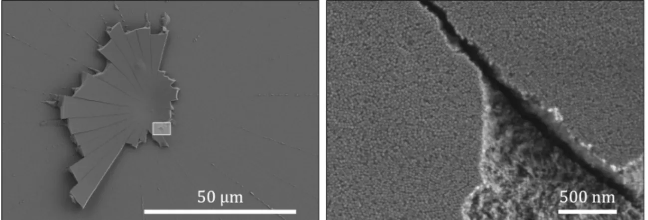
under consideration. In the Scanning Electron Microscope pictures shown in figure 3-1, we do not observe any clustering of particles (as opposed to a recent theory proposed by Ma and Jing [26]) or strong particle deformation. This is confirmed by higher magnification images as well.

(38)

Figure 3-1: Scanning Electron Microscope image of the deposit left attached on a glass slide after drying. The initial volume fraction is 0.23 and the initial contact radius is 𝑅0 ≈ 900µm. On the left, the very center of the deposit is visible, the rest

was detached due to the vacuum. On the the right is a close-view of this deposit. Individual nanoparticles are visible, and their diameter corresponds to the tabulated value 2𝑎 = 22 nm. No clustering of particles is visible.

3.1 Physical origin of the deposit formation and growth

3.1.1 Initiation of the deposit

The origin of the deposit formation is a flow that accumulates particles at the drop edge. This was first explained by Deegan [7] based on the following considerations:

∙ the evaporative flux 𝑗 is stronger at the edge

𝑗 ∼ (︃ 1 −(︂ 𝑟 𝑅0 )︂2)︃−𝜆 where 𝜆 = 𝜋 − 2𝜃 2𝜋 − 2𝜃 ≈ 0.5 for small 𝜃 (3.1)

∙ the contact line is initially pinned

If the contact line were free to move, it would simply recede. However, it is fixed in place. Furthermore, surface tension prevents deforming the interface out of a spherical shape. The only way evaporation can occur under these constraints is to have a flow from the center towards the edge of the drop. This flow in turn accumulates the particles at the edge: a deposit is formed. This mechanism is schematically shown in figure 3-2 (a).

(39)

Figure 3-2: Sketch of deposit initiation and growth. (a) Initiation of the deposit, which is the same at all volume fractions. A higher evaporative flux at the edge, shown by the black arrows, brings the particles to the edge. This pins the drop, which causes even more flow towards the edge. (b) Growth of the deposit for volume fractions higher than 0.06. The deposit is still wet. Air penetration inside the deposit would create a large amount of interface, as shown in the inset. Instead, water flows from the liquid cap through the deposit.

(40)

This mechanism is in agreement with flow solutions found analytically by Masoud and Felske [30] for sessile drops of pure liquids. Looking at their flow diagram, the first hypothesis is not necessary: even for a uniform drying rate, the flow lines point towards the edge if the contact line is pinned (figure 5.b in [30]). Considering the other hypothesis only, where the contact line would initially be free to move but the evaporative flux is stronger at the edge, leads to part of the drop liquid to be drawn towards the edge (figure 6.a in [30]). This could still induce pinning of the contact line if particles are present. This explains why a drop of a colloidal suspension will pin even on surface where a drop of pure water recedes.

3.1.2 Growth of the deposit

Deegan [7] argues that eventually, all particles will be deposited at the edge. However, he works in the range of very small volume fraction, 𝜑 ≪ 𝜑𝑔 such that Ω𝑑𝑒𝑝𝑜𝑠𝑖𝑡≪ Ω0.

The deposit ring that forms under these conditions is only a few particle diameters wide and the liquid cap remains pinned for the entire time of drying. More recent works [18] probe the deposition dynamics and the shape of the ring more precisely, but still only consider the low volume fraction range where the size of the deposit is much smaller than the drop size. This is no longer the case for higher volume fractions, and we here need to consider what happens in the deposit.

The scenario for the growth of the deposit is sketched in figure 3-2 (b). Once a deposit has been initiated, it will remain wet and water will evaporate from its surface. Indeed, for air to penetrate into the deposit it would need to create a large amount of water-air interface as capillary bridges appear between the particles, as shown in the inset of figure 3-2 (b). When the water in the deposit evaporates, a capillary pressure is generated which draws water from the liquid phase in the center through the deposit. We show in section 4.1.1 that this capillary pressure is sufficiently strong to pull water from the liquid cap.

(41)

3.2 Experimental methods

3.2.1 Optical profilometry

Experiments using an optical microscope allow us to determine the evolution of the liquid cap. To measure the height profile of the deposit, however, we use an optical profilometer (Keyence VK-X250), a laser scanning confocal microscope built to detect interfaces with an optical index mismatch.

The working principle is the following: a laser is directed at and reflected by an interface. The reflected light goes through a microscope lens, then through a pinhole placed at the focal distance 1/𝑓′ _{of the lens, before reaching a light intensity sensor.}

If the interface is also at a distance 1/𝑓′ _{of the lens, its image is in focus and all}

the light goes through the pinhole. If the interface is slightly closer or farther away than 1/𝑓′_{, some of the light rays get blocked at the pinhole and the light intensity}

decreases. By scanning in the vertical direction and recording the intensity maxima, the interface is identified.

Laser scanning confocal microscopy has the advantage that it can identify both solid-gas and liquid-gas interfaces, although we find that the latter can be tricky at times. Another advantage of this technique over contact profilometry is that multiple interfaces can be measured, as we will show in 3.2.3, but this must be done with caution. The counterpart of optical profilometry is that the sample must fit within the field of view of the objective.

The precision in the interface position is directly related to the smallest increment in lens position. This step size can be as low as 80 nm. However, the peak has to be clearly identified for this precision to be attained. As shown in figure 3-3, an interface appears as a peak in reflected light intensity with a finite width. If two interfaces are close, the peaks cannot be resolved [42]. The peak width sets a limit for the smallest measurable film layer thickness. This limit is dependent on the Number Aperture of the microscope and on the material properties. We also observe that the peak width depends on the intensity of the laser: at higher intensity, more light is scattered by the interface. This creates a challenge when multiple interfaces at different angles and

(42)

(a)

(b) (c)

Figure 3-3: (a) laser confocal profilometer Keyence VK-X structure. (b) Confocal working principle. (c) Raw experimental data, note the width of the intensity peaks. The second (green) interface is flat but appears deformed by the optical index mis-match. The first two figures are adapted from [19]. Copyright Keyence Corporation.

(43)

with different scattering properties need to be imaged: some light intensity maxima are too dim to measure, others saturate the light-receiving element.

Another issue in identifying the light intensity maximum arises when measuring multiple interfaces through a sample, where the sample microstructure can create strong variation in the intensity curve.

Finally, confocal profilometry remains a point measurement technique. Even with a very fast X-Y scanning optical system, precise measurements in 3D often take minutes to complete. Techniques built on white light interferometry have faster ac-quisition rates because they cover the entire plane in one image, but their analysis is more involved and difficult to validate with complex materials.

We use the profilometer for two sets of measurements, outlined in the following subsections.

3.2.2 Determination of height profile during drying

Capturing the height profile during drying has multiple advantages. We can estimate the rate at which deposit grows, and probe if the deposit changes shape after its creation. When the deposit is still in contact with the substrate, we can measure its thickness more accurately.

However, drying occurs quite fast in our experiments. To shorten the image acquisition times we measure the profile along a single line, as shown in figure 3-4. In these settings the optical profilometer captures the height profile with a resolution of 0.5µm in 1 - 2 s, with an average time between measurements of 8 s.

(44)

Figure 3-4: Profile measurement during drying for 𝜑0 = 12 % (single crack regime).

(a) Top: view of the entire drop with measured area outlined. Bottom: optical image recorded during the measurement at 𝑡 = 55 s. Profile measurements are made along the dotted line. (b) Profiles measured at different times. The liquid cap recedes, leaving a deposit behind.

(45)

3.2.3 Post-drying determination of height profile

To access the complete deposit thickness, we also measure the deposit profile after drying and bending. Furthermore, the relative humidity cannot be controlled during optical profilometry experiments due to the geometry of the instrument. To obtain the shape of the deposit at higher relative humidity, we need to measure it after drying.

To capture the upper and lower interfaces separately, the magnification is increased and up to five measurement windows are stitched together to reconstruct the profile of a single petal. An example of such a measurement is shown in figure 3-5.

For the lower interface, the measured position is shifted up compared to the real one: the deposit appears thinner than it actually is. This optical effect is caused by the index of refraction of the deposit. Light reflected from the lower interface goes through the deposit - air interface, and is focused at a distance different from 1/𝑓′_.

The scaling factor between the real and measured distances is approximately equal to the index of refraction [21] and can be determined from the data during drying. However, it adds uncertainty to the measurement.

In the following, we report the deposit thickness by subtracting the upper and (corrected) lower interface 𝑧-position for the same 𝑥. This is valid as long as the normal to the deposit is close to the vertical, that is, for small bending angles where cos 𝜃 ≈ 1, which is the case in our experiments.

(46)

Figure 3-5: Profile measurement after drying for 𝜑0 = 8 % (single crack regime).

(a) 3D visualization of the lower and upper interfaces. (b) Four measurements are stitched together to obtain the profile over the entire length of the petal. The dashed line is the 𝑟 axis in (c) and (d). (c) 2D visualization of the lower and upper interfaces along the dashed line in (b), corrected for the optical scaling factor. The data is mirrored around 𝑟 = 0 for better visualization. (d) Deposit profile obtained from (c) (in blue) and obtained from measurements during drying (in red). We obtain very good agreement given that different petals of the same drop are measured in each case. The data is mirrored around 𝑟 = 0 for better visualization.

(47)

3.3 Deposit shape

Using a combination of the two types of measurements outlined in section 3.2, we examine the final deposit shapes for various volume fractions.

3.3.1 From infinitesimal to large particle volume

We aim to elucidate the transition from the coffee-ring regime with a deposit width 𝑤 ≪ 𝑅0, to the single crack regime with 𝑤 ≈ 𝑅0.

Let us start with the coffee-ring regime for a volume fraction 𝜑0 = 10−4. The

liquid cap remains pinned for the duration of drying1_{. At late time, the contact angle}

approaches zero (figure 3-6), and the final layer of water disappears. We observe a ring of width 𝑤 = 65 µm. If we assume an uniform height across this width, and a final volume fraction 𝜑𝑔 ≈ 0.6, we expect an average deposit height ℎ = 120 nm.

Taking line averages parallel to the edge, we measure a value of 500 nm at the very edge, dropping down to 100 nm then 50 nm as we move towards the drop center the deposit.

We emphasize two observations: first, these values are close to the diameter of the particles 2𝑎 = 22 nm. The continuum assumption breaks down as the height become close to the size of the constituents. We observe a complex microstructure with aggregates. Secondly, the deposit is thicker at the outer edge than at the inner

Figure 3-6: Final moments of drying for a drop of initial volume fraction 𝜑0 = 10−4

(coffee-ring regime). The pictures are taken 7 s apart. The contact angle in the first picture is estimated as 1 - 2∘ _{from profile measurements.}

1_{In some experiments, slip-stick motion occurs where the liquid cap unpins, recedes, then pins} again, leaving characteristic concentric rings. This has been well-studied in the literature, see eg [33]

(48)

edge.

An increase in the volume fraction by a factor of ten, to 𝜑0 = 10−3, brings us to

the ring-crack regime. The resulting height profile is shown in figure 3-7. We observe a very sharp drop at the inside edge. Furthermore, the deposit is here thickest at the inside edge, contrary to the coffee-ring situation. Beyond that edge, we see a rough, non-uniform coverage with an average thickness close to the single particle diameter. This thin coverage extends for about twice the deposit width.

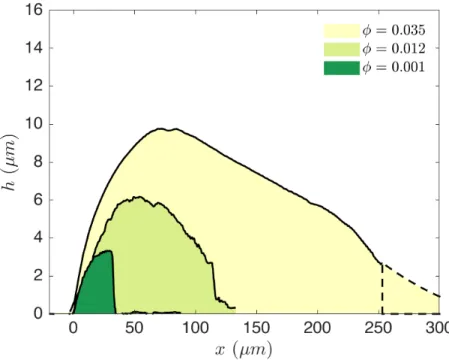
Figure 3-7: Deposit profiles measured in the ring-crack (𝜑0 = 10−3) and double-crack

regimes (𝜑0 = 1.2 × 10−2 and 3.5 × 10−2). 𝑥 = 𝑅0− 𝑟 is sketched in figure 3-4.

A further increase of the volume fraction by a factor of ten brings us in the double-crack regime. The liquid cap recedes and the deposit width becomes larger. On the deposit side, we still see a bump at the deposit edge. However, instead of dropping off abruptly, the deposit thickness gradually decreases. Indeed, the deposit covers the entire drop, as evidenced by the cracks that form in it.

We note that the transition between these two deposition profiles, a sharp drop off and a rolling hill, is not necessarily equal to the transition between the ring-crack and double-crack regime. In fact we expect some ring-crack drops to have a smooth deposit shape, which simply does not crack the entire way. This is because to form

(49)

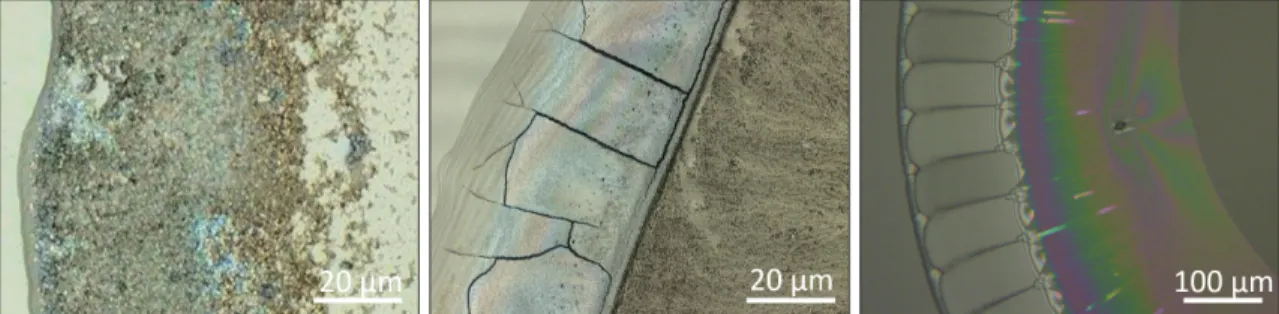
Figure 3-8: Laser-enhanced optical images of a coffee-ring (𝜑0 = 10−4), ring-crack

(𝜑0 = 10−3), double-crack (𝜑0 = 1.2 × 10−2).

cracks, the deposit must be above a critical thickness [43]. Indeed, we sometimes see ring-cracks where the liquid cap recedes without any crack, until the receding liquid pools up around a defect and form cracks only there. We will consider the changes in crack pattern in more detail in section 4.4.

3.3.2 Deposit thickness in the single-crack regime

Let us now examine the shape of the deposit in the single-crack regime, for 𝜑0 > 0.06.

As we move from the outside to the inside of the drop, the thickness initially increases before reaching a slowly varying plateau. In some drops, we observe a second "bump" or local maximum before the thickness drops down to zero. The profile close to the center cannot be measured by our experiments because it is strongly curved and the intensity peaks due to the upper, lower, and substrate interfaces cannot be separated. However we note that there is a small circular region of characteristic size 100 µm at the center of the deposit which is very thin. We did not further study this feature, and the change in deposit volume it causes is negligible.

The thickness varies in complex ways, however we remember that ℎ ≪ 𝑅0, so any

variation in thickness 𝑑ℎ/𝑑𝑟 will be very small. In the following we will assume that ℎ is constant away from the drop center and the drop edge.

If we assume a constant deposit height, we obtain the following expression for the height from conservation of particle volume, 𝜑0Ω0 = 𝜑𝑔Ω𝑑 :

ℎ = 𝜑0 𝜑𝑔

Ω0

(50)

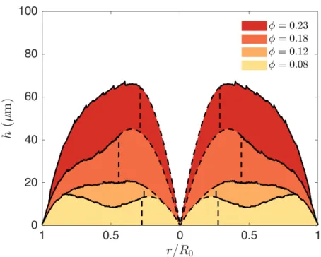
Figure 3-9: Deposit profiles measured in the single-crack regime. The dotted line is a continuation of the profile by a second order polynomial. The x-axis is scaled by the initial drop radius.

3.3.3 Maximum height as a function of volume fraction

For a constant deposit height, we expect a linear relationship between the volume fraction and the deposit height. However, if the deposit has a wedge shape with a linear increase in thickness, ℎ ≈ 𝑤 sin 𝜃, the deposit will cover a ring of width 𝑤 ∼ ℎ. For 𝑤 ≪ 𝑅0 we obtain Ω𝑑= 1 2𝑤ℎ𝑅0 = 1 2 sin 𝜃ℎ 2_𝑅 0 = Ω0 𝜑0 𝜑𝑔 (3.3) . Thus we would expect ℎ ∼ √𝜑0. The same scaling should hold if most of the

deposit volume is contained inside a bump of width 𝑤, as is the case in the double-crack regime.

We observe a good agreement with these scalings in figure 3-10. The value of the linear slope of ℎ versus 𝜑0 for the single-crack regime is close to the one predicted

from equation 3.2.We note, however, that the geometrical factor sin 𝜃 must be divided by 150 to obtain a good fit from equation 3.3, which indicates that the width is much

(51)

Figure 3-10: Deposit height versus initial volume fraction. We report the maximum deposit height. The dashed line represent the transition between the ring-crack, double-crack and single-crack regimes. A power law with exponent 1 is observed for the single-crack regime, and with exponent 1/2 in the double-crack regime.

larger than that expected if the deposit had a simple wedge shape: 𝑤 ≈ 150/ sin 𝜃 ℎ. Furthermore, data in the ring-crack regime at 𝜑0 = 10−3 is not in agreement with

this scaling. A change in the geometrical factor 𝑤/ℎ would explain this variation. At these low volume fractions, the mass of Ludox used to prepare the solution is very small and the uncertainty on the volume fraction grows.

3.3.4 Determination of the deposit volume

Since we have access to the deposit profile, we can integrate the profile to get a measurement of the deposit volume and the deposit volume fraction using

𝜑𝑔 = 𝜑0

𝑔(𝜃)𝑅3₀ ∫︀𝑅0

0 2𝜋𝑟ℎ(𝑟)𝑑𝑟

(3.4) However, the results are too spread to be useful. The main roots for error are:

∙ the small variation in contact angle 𝜃 leading to an uncertainty on the initial volume,

(52)

∙ drops that are not symmetric,

∙ the position of the measurement line (dashed line in figure 3-4). We must chose the position quickly to start measuring, and can end up off-center. This leads to an error in the values of 𝑟 and makes the assumption of symmetry no longer valid.

While the ratio between the initial and total deposit volume is off, we will see in the next section that the volume increase with time provides important information.

3.4 Deposit growth

The deposit growth is very different depending on the initial volume of particles in the drop. For drops in the coffee-ring and ring-crack regimes, the deposit remains too small to follow its temporal evolution. We therefore focus on the double-crack and single-crack regimes, where deposit growth is visible.

As discussed in section 3.1, the deposit remains wet as a flow from the liquid cap compensates for the evaporation. We will now discuss this process in a more quantitative way.

3.4.1 Model for deposit growth

The deposit does not change thickness once it is formed, as seen in figure 3-4. The deposit growth is therefore entirely defined by two functions of a single variable: h(r), the deposit thickness profile, and rc(t ), the liquid cap radius. The deposit width is

then 𝑤 = 𝑅0− 𝑟𝑐.

Assumptions To start with, we do not make any assumption on ℎ. The only assumption we make is that the deposit volume fraction is constant:

(53)

Volume conservation We start by writing the volume conservation for the total volume and for the volume of particles:

𝑑Ω𝑐𝑎𝑝+ 𝑑Ω𝑑𝑒𝑝𝑜𝑠𝑖𝑡 = −𝑉𝐸𝑆𝑑𝑡 (3.6)

𝜑𝑔𝑑Ω𝑑𝑒𝑝𝑜𝑠𝑖𝑡+ 𝑑 (𝜑𝑐𝑎𝑝Ω𝑐𝑎𝑝) = 0 (3.7)

we combine and integrate these equations to obtain

Ω𝑑𝑒𝑝𝑜𝑠𝑖𝑡+ Ω𝑐𝑎𝑝= Ω0− 𝑉𝐸𝑆𝑡 (3.8)

Ω𝑐𝑎𝑝(𝜑𝑔 − 𝜑𝑐𝑎𝑝) = Ω0(𝜑𝑔− 𝜑0) − 𝜑𝑔𝑉𝐸𝑆𝑡 (3.9)

To close the system, we need a third equation. This equation must be related to the physics of deposition at the liquid cap - deposit interface. We stated that the deposit grows because of a flow from the center to the deposit. As the particles are small and the flow is slow, the particle velocity will be equal to the fluid velocity, except for the contribution of Brownian motion governing the diffusion of the particles. It follows that if we neglect diffusion, flow effects alone will not cause any change in the liquid cap volume fraction. An element of fluid 𝑑𝑉– with 𝜑𝑐𝑎𝑝𝑑𝑉– particle volume and

(1 − 𝜑𝑐𝑎𝑝)𝑑𝑉– water volume will be drawn to the liquid cap boundary and deposit its

particles there while its water penetrates the deposit.

The Peclet number compares the effects of diffusion and advection. The flux of water scales as 𝑉𝐸𝑅20 and goes through the liquid cap of height 𝐻 at a speed 𝑈, so

𝑈 𝑅0𝐻 ∼ 𝑉𝐸𝑅02. This gives us 𝑃 𝑒𝑅 = 𝑈 𝑅0 𝐷0 = 𝑉𝐸𝐻 𝐷0 ≈ 2 − 6 (3.10)

Where 𝐷0 = 2 × 10−11m2s−1 is the diffusion coefficient of the particles in water

estimated from the Stokes-Einstein equation. Thus we neglect diffusion in the radial direction and we assume

(54)

Which closes the system. We obtain a linear growth in deposit volume: Ω𝑑𝑒𝑝𝑜𝑠𝑖𝑡 = 𝑉𝐸𝑆

𝜑0

𝜑𝑔− 𝜑0

𝑡 (3.12)

3.4.2 Comparison with experiments

We integrate 2𝜋ℎ𝑟𝑑𝑟 from 𝑟 = 𝑅0 to 𝑟 = 𝑟𝑐(𝑡) to obtain Ω(𝑡). Ω(𝑡) is plotted for

two drops in figure 3-11, in the double-crack and single-cracks regimes. We observe a linear increase in deposit volume for all the experiments spanning a range of initial volume fraction 𝜑0 = 0.03 − 0.23. This confirms our hypothesis 3.11 that the liquid

cap volume fraction stays close to its initial value.

The fit always predicts that the deposit has a volume of 0 at a finite time, indi-cating that deposition is slower at the beginning and/or that deposition only starts after a certain time.

We further measure the volume growth rate ˙Ω = 𝑑Ω/𝑑𝑡 of the deposit for different drops. All our experiments were conducted at the same relative humidity 𝑅𝐻 = (15 ± 1) %. In figure 3-12, we plot ˙Ω/(𝑉𝐸𝑆) against volume fraction and the model

prediction. We obtain a good agreement using the value of 𝜑𝑔 = 0.6and a drying rate

𝑉_𝐸* = 950 nm s−1 (20 % larger than our estimate in section 2.3). The highest volume fraction experiment deviates from the trend: more experiments are needed.

3.4.3 Application to the liquid cap retraction

From our expression for the deposit volume increase (equation 3.12), we can plug in a deposit shape ℎ(𝑟) to obtain 𝑟𝑐(𝑡) and 𝑤. If we consider a small change in liquid

cap radius 𝑑𝑟𝑐 we can write

𝑑Ω𝑑𝑒𝑝𝑜𝑠𝑖𝑡 = ℎ(𝑟𝑐)2𝜋𝑟𝑐(−𝑑𝑟𝑐) = 𝑉𝐸𝑆 𝜑0 𝜑𝑔− 𝜑0 𝑑𝑡 or 𝑑𝑟2 𝑐 𝑑𝑡 (𝑡) = − 𝑉𝐸𝑆 𝜋ℎ(𝑟𝑐(𝑡)) 𝜑0 𝜑𝑔− 𝜑0 (3.13)

(55)

Figure 3-11: Temporal evolution of the deposit profile and deposit volume for two drops of different initial volume fraction. (a) and (b) 𝜑0 = 3.5 % (double-crack

regime). The deposit covers the entire drop. (c) and (d) 𝜑0 = 11.7 % (single-crack

regime). The green line corresponds to the model prediction for Ω0 = 𝑔(𝜃)𝑅30 and

(56)

Figure 3-12: Deposit volume growth rate normalized by total drying rate versus initial volume fraction. The model corresponds to equation 3.12.

Once again, to get ℎ(𝑟) we need one more equation. Parisse and Allain [34] find that by considering flow inside a spherical cap they are able to derive a simplified solution which gives a good fit for the outside edge. To obtain the complete solution, one must solve for the flow inside the liquid cap, considering both the particles and the solvent. This has been done in by Routh for the case of films [37] at large volume fraction and by Fischer for the case of droplets [10] at small volume fraction. Routh in particular solves for a large volume fraction in the lubrication approximation. His model accounts for particle motion independently from the solvent due to osmotic pressure, but neglects horizontal particle diffusion. However, all of those models need to be solved numerically.

We see in figure 3-9 that, in the single crack regime, ℎ(𝑟) does not vary considerably away from the drop edge and center. To see if those small variations affect the liquid cap retraction we plot the square of the liquid cap radius 𝑟2

𝑐 versus time for various

drops in figure 3-13.

We see that a linear fit describes the data well, with some variations that can be attributed to slow changes in the deposit height. We note here that we do not have

(57)

Figure 3-13: The square of the liquid cap radius 𝑟2

𝑐 versus time for various initial

volume fractions (single-crack regime) and RHs. Insert: 𝑟𝑐/𝑅0 versus time for

Drying of colloidal suspension drops : pattern formation and mechanical deformation

Drying of colloidal suspension drops:

pattern formation and mechanical deformation

by

Paul Lilin

Titre d’Ingénieur, École polytechnique (2018)

Submitted to the Department of Mechanical Engineering

in partial fulfillment of the requirements for the degree of

Master of Science in Mechanical Engineering

at the

MASSACHUSETTS INSTITUTE OF TECHNOLOGY

May 2020

c

○ Massachusetts Institute of Technology 2020. All rights reserved.

Author . . . .

Department of Mechanical Engineering

May 15, 2020

Certified by . . . .

Irmgard Bischofberger

Assistant Professor

Thesis Advisor

Accepted by . . . .

Nicolas Hadjiconstantinou

Chairman, Department Committee on Graduate Theses

Drying of colloidal suspension drops:

pattern formation and mechanical deformation

by

Paul Lilin

Abstract

Acknowledgments

Contents

List of Figures

Chapter 1

Introduction

1.1

Drying of sessile drops

1.2

Colloidal suspensions

1.3

Drying of colloidal suspensions

1.3.1

Vertical drying

1.3.2

Horizontal drying

1.4

Pattern formation in drops

1.5

Overview: blooming flowers

Chapter 2

Evaporation process

2.1

Methods

2.1.1

Colloidal suspension

2.1.2

Substrate

2.1.3

Drop deposition

2.1.4

Ambient conditions

2.2

Mass measurements

2.2.1

Estimate of evaporative flux 𝑉

2.2.2

Estimate of deposit volume fraction 𝜑

2.3

Total drying time

2.3.1

Estimate of evaporative flux and deposit volume fraction

Chapter 3

Formation of a particle deposit

3.1

Physical origin of the deposit formation and growth

3.1.1

Initiation of the deposit

3.1.2

Growth of the deposit

3.2

Experimental methods