Intergenerational Equity by Educational Attainments in France

(1)

HAL Id: halshs-02549807

https://halshs.archives-ouvertes.fr/halshs-02549807

Preprint submitted on 21 Apr 2020

HAL is a multi-disciplinary open access archive for the deposit and dissemination of sci-entific research documents, whether they are pub-lished or not. The documents may come from teaching and research institutions in France or abroad, or from public or private research centers.

L’archive ouverte pluridisciplinaire HAL, est destinée au dépôt et à la diffusion de documents scientifiques de niveau recherche, publiés ou non, émanant des établissements d’enseignement et de recherche français ou étrangers, des laboratoires publics ou privés.

Intergenerational Equity by Educational Attainments in

France

Hippolyte d’Albis, Ikpidi Badji

To cite this version:

Hippolyte d’Albis, Ikpidi Badji. Intergenerational Equity by Educational Attainments in France. 2020. �halshs-02549807�

(2)

WORKING PAPER N° 2020 – 19

Intergenerational Equity by Educational Attainments in France

Hippolyte d’Albis Ikpidi Badji

JEL Codes:

(3)

1

Intergenerational Equity by Educational Attainments in

France

1

Hippolyte d’ALBIS2_{and Ikpidi BADJI}3

Abstract: This article analyses the development of inequalities across ages and

generations in France using a pseudo-panel developed from the successive waves of the French Household Expenditure Survey that took place between 1979 and 2011. The standard of living of individuals, evaluated using individualized disposable income or private consumption, including housing expenditure and imputed rent, is decomposed by sex and educational attainment. The estimation of Age-Period-Cohort models reveal that men with lower education attainments who were born after 1950 experienced a significant decline in disposable income with respect to those who were born between 1918 and 1950. Conversely, when the whole population of men is considered, no decline in disposable income is observed. The evolution is rather different for women: those with lower education attainments did not experienced any decline whereas the whole population of women benefitted from a strong increase in disposable income across generations.

Keywords: Intergenerational Equity; Age-Period-Cohort models; Qualifications.

1_{We thank the special editor of this issue and the anonymous reviewers for their careful reading of our} manuscript and their insightful suggestions and comments. This research was supported by the Agence nationale de la recherche within the JPI MYBL framework (Award no. ANR-16-MYBL-0001-02).

2_{Paris School of Economics and CNRS. Corresponding author. Address: 48 boulevard Jourdan, 75014 Paris,} France. Email: [email protected]

3_{Economix, Université Paris Nanterre. Address: Bâtiment G - Maurice Allais, 200 avenue de la République, 92001} Nanterre cedex, France Email: [email protected]

(4)

2 Introduction

Age dependency ratio in France has continuously increased in France since the mid 1980’s. The ratio of dependents (people younger than 15 or older than 64) to the working-age population (those ages 15-64), is now above 60% against 50% in 1986. This change in the demographic structure is often seen as a potential threat for intergenerational equity as the numerous cohorts who were born after the Second World War require large inflows of public transfers to finance their pensions and health care. In d’Albis and Badji (2017), we nevertheless showed that there was no decline in standard of living across generations in France and, in particular, that the baby-boom cohorts did not enjoy a more favorable position than the cohorts that followed them. In this article, we continue the analysis of intergenerational inequalities in France by adding two important dimensions. The first is gender, to capture the effect of the strong increase in the participation of women to the labor market since the Second World War. The second is education, which also tremendously increased across cohorts over the period.

Intergenerational equity is not a simple concept to evaluate mainly because it is not straightforward to define. An egalitarian situation across cohorts might not be desirable as most people would be happy to see their children with better standard of living. Therefore, a general increase of the standards of living across generations, which is an intergenerational inequality by definition, cannot be rejected on the ground of fairness. This induces an asymmetry in the comparisons of a generation with the preceding and the following ones. In a nutshell, there is a consensus to say that equity between generations is ensured as long as their standard of living does not deteriorate (Stavins et al. 2003, Arrow et al. 2004). This analysis across generations translate to the comparison across ages. Over the life-cycle, a decline in consumption is often perceived as non-desirable. Whatever the age profile of income, one should be able to allocate her resources to ensure a non-declining consumption. In the analysis we

(5)

3

present below, we therefore focus our attention on whether standards of living are declining for younger generations and over the life-cycle.

Technical difficulties also arise when intergenerational equity is evaluated. One would ideally measure “wellbeing”, which is complicated as it is surely a composite variable that includes subjective measures. Economists then tend to use consumption as a proxy whereas national statistical institutes commonly use disposable income as it is better measured in surveys. In this article, we use both of them and consider them as measures of the standard of living. Another technical difficulty hinges on the fact that ideally, one would have access to panel data following individuals of different generations over their life-cycle. But for most countries, including France, such panels no not exist. We therefore use the seven editions of the French Expenditure survey, carried out between 1979 and 2010, which we rework in order to develop a pseudo-panel to follow different cohorts throughout their lifecycle. This gives us 407 cohort observations, comprising an average of 288 individuals.

The main novelty of our study is to assess the role of educational attainment in intergenerational equity. Due to sample size limitations, we provide a rough evaluation of educational attainment per cohort by simply identifying individuals who have not completed their secondary education. In the French educational system, at the end of the secondary system, students pass a national exam, named Baccalauréat, which permit to obtain a diploma that generally gives access to university studies. The evolution of the share of Baccalauréat graduates within cohorts has skyrocketed from around 10% in the 1960’s against nearly 80% today. It reveals a tremendous increase in the possibility access higher education in France, which translates in the proportion of university students (Duru-Bellat and Kieffer 2008). The share of Baccalauréat graduates is thus an indicator of the evolution of the qualifications in France, although it is imperfect —as any indicator. In particular, the creation of a vocational Baccalauréat, whose graduates have lower chances than other to complete tertiary

(6)

4

education, soften the picture. Nevertheless, the share of persons who accessed tertiary

education and get a university diploma increased over the period.4_{Luckily, the}

information on whether individuals have passed the Baccalauréat or not is provided in the surveys we use. By comparing, across cohorts, persons without a Baccalauréat, we are thus able to provide a statement with a control for the increase in qualifications. This is also meaningful as intergenerational comparisons made by everyone may implicitly assume a stable qualification structure: non educated sons may compare themselves with their non-educated fathers, while it would be perceived as obvious that education improve the standard of living across generations.

Using an Age-Period-Cohort model and the identification strategy of Deaton and Paxson (1994), we show that women’s position has considerably improved while men’s has stagnated for all cohorts born after the Second World War. When we restrict to the population without a Baccalauréat, we show that men who were born after 1950 experienced a significant decline in disposable income with respect to those who were born between 1918 and 1950. Conversely, women without a Baccalauréat did not experienced such a decline. We conclude that despite economic growth, equity across generations of less educated men was not achieved for cohorts born after 1950 and that cohorts born between 1918 and 1950 were relatively favored. We moreover show that the relative economic position (as measured by disposable incomes) of men generally decreased from one generation to another, ant that the decline is particularly strong for men without a Baccalauréat.

This article is in the continuation of a broader project based on the development of National Transfers Accounts (NTA, hereafter) for France. The ambition of the NTA is to measure all public and private transfers between ages and generations by providing a breakdown of all relevant variables of the National Accounts by age, and possibly by

4_{As an illustration, Duru-Bellat and Kieffer (2008) computed that the percentage of access to tertiary education} rose from 27.7% for the 1962-1967 cohorts to 53.2% for the 1975-1980 cohorts.

(7)

5

gender and education. In France, the life-cycle deficit (i.e. the difference between labor income and consumption) was presented in d’Albis et al. (2015). More recently, d’Albis et al. (2019) showed that over the period 1979-2011, the share of consumption per elderly that was financed by the State did reduced. Over the period, the elderly have relied increasingly on themselves to finance their consumption whereas the youth increasingly relied on the State and their family to finance their own consumption. These results suggest that the major demographic changes that took place in France during this period was not made at the expense of the youth. This analysis however relies on repeated cross sectional observations and the life cycle dimension is not taken into account. In d’Albis and Badji (2017) and in the present article as well, we are using the same data sources in order to provide a complete comparison of the standard of living across ages and generations using Age-Period-Cohort models. This analysis is better suited to determine whether intergenerational equity deteriorated over the last 40 years.

The rest of the paper is organized as follows. Section 2 presents the database, the main variables we consider and the estimation strategy based on Age-Period-Cohort models. Section 3 presents our estimates of the evolution of standard of living across age groups and across cohorts. Section 4 concludes.

2 Data, Descriptive Statistics and Estimation Strategy

2.1 Standards of Living in French Expenditure Surveys

We use the French Household Expenditure surveys (Budget de famille, named BdF hereafter) conducted in 1979, 1984, 1989, 1995, 2000, 2005 and 2010 by the French Statistical Institute, INSEE. These surveys were carried out among 10,000 households with the aim of reconstituting all household accounts by gathering information on their

(8)

6

income and expenditure. It is worth noting that, in the survey, a household refers to a group of people who ordinarily share a dwelling and have a shared budget.

Standard of living are evaluated with the help of two main variables. First, disposable income --defined as the income after deduction of taxes and social security contributions-- is used. It includes: (i) working income: salaries, self-employed income, etc.; (ii) income from household worth: dividends, interest, rent, etc. to which we add the imputed rents; (iii) social security benefits, including pensions and unemployment benefits; (iv) current transfers, particularly insurance indemnities minus premiums and transfers between households. As a robustness check, we also compute the disposable income excluding imputed rent (as they are not directly observed in the first waves of the surveys). Second, we use private consumption at the individual level. This is the sum of the 12 consumption items given by the Classification of Individual Consumption by Purpose. It excludes taxes, major maintenance work and loan repayments, but includes imputed rent. As a robustness, we also use a modified private consumption that is computed without all expenditures related to housing (such as rents, imputed rents, etc.).

Note that the 1979 to 1995 surveys do not provide figures for imputed rents, which were thus estimated using the characteristics of housing as in d’Albis et Badji (2017).

The imputed rent Ri of homeowner i is calculated using the following equation:

𝑅_𝑖 = 𝑒𝑥𝑝(𝛽𝑋𝑖+𝜀𝑖)

where Xi is a vector of key variables (region, urban units, surface area, number of

rooms, housing type, etc.) of a rent equation for observation i, where β is the vector of the estimated coefficients of the rent equation and where the ε stand for the residuals. In order to obtain correct rent distribution, the imputed residual must have the same distribution as the residuals taken from the rent equation. As the rent equation

(9)

7

residuals are heteroscedastic and non-Gaussian, they cannot be expressed as a normal distribution. The appropriate residual imputation method is the Hot Deck method, which involves randomly selecting an estimated residual using the estimation from the rent equation. This residual is then imputed to housing that are similar to the one from which we selected the estimation residual and for which we have to calculate the imputed rent.

In the BdF surveys, the consumption is declared at the household level. Contrarily to d’Albis and Badji (2017), we individualize the variables and split them among the household members using the NTA rule, which gives a weighting that worth 0.4 to any individual under age 4 and that linearly increases with age till age 20 where it reaches 1. The BdF surveys moreover provide some incomes at the household level (such as property incomes, imputed rents, family benefits, transfers between households direct

taxes paid) and others at individual level. We individualize the variables as follows5_.

Property income, transfers between households, direct taxes and family benefits are allocated equally between the household head and his or her spouse. Imputed rents are allocated using the NTA rule. We have chosen to treat differently imputed rents from other property incomes as children directly benefit from living in the housing own by their parents. This assumption has no consequence on our main qualitative results as our estimates are done for variables computed with and without imputed rents.

In order compare data within a consistent time frame, we adjust survey data to the French System of National Accounts aggregates. This adjustment is similar to the one carried out for the NTA (d’Albis et al. 2015) and aims to equal the aggregate disposable income of individuals with National Accounts aggregates. Before adjustment, we corrected differences in coverage and concept between the BdF survey and National Accounts as much as possible. The main difference comes from the under-declaration

5_{Note that we do not follow the recommendations made by the NTA (United Nations 2013), which suggest to} allocate property incomes to the household head only. Since such an allocation would bias our results by gender, we have chosen a more realistic one.

(10)

8

or non-declaration of some consumption and income in surveys. Moreover, The BdF survey only collects the income and consumption of individuals residing in France in ordinary households (i.e. excluding households residing in mobile or communal dwellings), whereas the National income considers all households. In addition, the BdF survey covers the consumption of French residents abroad, but does not include the consumption of foreign tourists in France. Finally, all the variables we consider are deflated using the consumer price index provided by INSEE.

The rescaled individual variables are then split by sexes and by educational attainment. In particular, we consider individuals with lower educational attainments by grouping all those who do not have the Baccalauréat, which is the national diploma that allows students to pursue university studies. This category is relevant in the French context as persons without a Baccalauréat face a higher risk of unemployment, poorer working conditions and weaker remunerations.

First, according to the recent literature (Amossé and Chardon 2006, Jauneau 2009, Le Rhun and Pollet 2011), the access to the labor market strongly depends on the educational attainment. For example, in 2010, the unemployment rate between one to four years after the completion of the studies was 11% for the university graduates, 23% for those who only have a Baccalauréat and 44% for those who had no qualification at all. After five years, the difficulties remains for the latter as their unemployment rate ranges between 20 and 30%.

Moreover, Le Rhun and Pollet (2011) show that the situation of those without a Baccalauréat has deteriorated over the last forty years. Between 1979 and 1985, their unemployment rate doubled from 21% in 1979 to 42% in 1985. The rate then reduced till 1989 when it stabilized to about 30% for three years. After 1992, the unemployment rate increased again and reached 45% in 1999. In comparison, during the same period, the employment rate of the whole population increased by 5 percentage points. During

(11)

9

economic crisis, such as the 2008-2009 crisis, the less qualified are more impacted by the economic downturn as their work contracts are more precarious and as recently qualified persons are accepting jobs for which they are overqualified.

Concerning the working conditions, it has been shown that persons without a Baccalauréat have less stable position as they are more likely to accept short term contracts of employment and part-time jobs. According to Jauneau (2009), in 2007, 23% of the employees without a Baccalauréat were employed in short-term contracts against 14% for the whole population of employees. Moreover, the share of part-time jobs is 32% for those without a Baccalauréat against 18% for the rest. They are also more likely to be in constraint under-employment, meaning that they would like to work more. Even if one controls for age and sex, constrained under-employment is higher for persons without a Baccalauréat.

The wage gap between qualified and non-qualified employees was rather stable from 1996 to 2002 and amounted to 35% (Amossé and Chardon 2007). Once controlled for age, sex and part-time jobs, Jauneau (2009) estimates that the gap between non-qualified employees and the rest of the whole population of employees reached 44% in 2006. This partly translate to the disposable income with a gap that is estimated to reach 25% in 2006. The reduction of the gap can be explain by the socio-fiscal system.

2.2 A Pseudo Panel

In order to dissociate the effects of age, cohort and period, individual data can be used provided that one has panel data that follow individuals throughout their entire lifecycle. Since our data are cross-sectional, it is necessary to build pseudo-panels that group individuals belonging to the same cohort. Otherwise, the estimations could be biased (Deaton 1985, Guillerm 2017). We defined our cohorts using the “date of birth” variable, and thereby constituted 79 annual cohorts. The first cohort is made of

(12)

10

individuals who were born in 1901 and the last cohort is made with those who born in 1979. Our pseudo-panel includes 407 observations of our cohorts, because not all cohorts are observed in each survey. The sizes of cohorts, which depend on the considered sample, are reported in Table 1. Small sizes mainly concern older cohorts, and particularly men as their life expectancy is lower. Obviously, among the population without a Baccalauréat, the sizes are smaller and represent on average 76% of the mean size of cohorts. Conversely, we see that the observed size of the population with a Baccalauréat is too small in order to produce robust estimates. The proportion of persons without a Baccalauréat within a cohort obviously decreases with the cohort birth date. According to the 2010 survey, the proportion was around 87% for the cohorts 1926-35, 70% for the cohorts 1946-55, and 45% for the cohorts 1966-75. The evolution for each sex reveals a striking reversal: the proportion was larger among women than for men (88% vs 85%) for cohorts 1926-35, was equal for cohorts 1946-55 and became lower among women (43% vs 49%) for cohorts 1966-75.

Table 1. Size of observed cohorts

Both sexes Men Women

All N.B. All N.B. All N.B.

Mean size 288 220 138 107 150 113

Minimal size 39 31 15 11 24 18

Maximal size 574 524 277 264 305 277

P100 94% 90% 72% 51% 80% 59%

Note: N. B. stands for “No Baccalauréat” and P100 stands for “Proportion of cohorts whose size is greater than 100 individuals”.

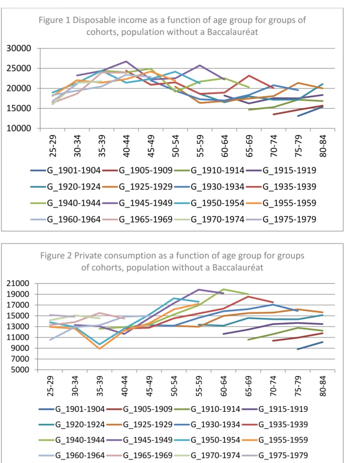
Reprocessed data may be presented diachronically. For instance, Figures 1 and 2 represent the disposable income and the private consumption by age for 16 generations of persons who do not have the Baccalauréat. These generations were established using the 79 annual cohorts defined above. A generation’s relevant

(13)

11

variable is defined using the mean of five consecutive cohorts, except for the first generation which consists of 4 cohorts. Two main observations can be made. First, both profiles display a hump-shaped function of age with a pick around 40 year-old for disposable income and around 60 year-old for private consumption. Second, for most ages and generations, an increase in both variables that benefit to the younger generations. Profiles for the whole population are generally similar except for the pick ages that may differ (see Figures II and IV in d’Albis and Badji 2017).

Figure 1 about here

Figure 2 about here

To sum up, we built pseudo-cohorts for 24 variables: our four estimates of the standard of living (disposable income, disposable income without imputed rents, private consumption, private consumption without housing expenses) which are decomposed by sex and educational attainment into six categories, as indicated in Table 1. For discussion purposes, we have also created a set of additional variables: they are the shares of disposable income of a subpopulation within the disposable income of the whole population. In particular, we computed the share of disposable income of men and the share of disposable income of men without a Baccalauréat. As for the previous variables, those shares are cohort and time specific.

2.3 Estimation Strategy

The simultaneous introduction of the age, cohort (i.e. date of birth) and period variables in the estimation creates a collinearity problem due to the fact that the survey year is equal to the sum of the age and cohort variables. As discussed in d’Albis and Badji (2017), various solutions were proposed in the literature to resolve this problem. We follow the most common strategy due to Deaton and Paxson (1994) that imposes

(14)

12

restrictions on the estimated parameters. In this approach, it is assumed that period effects sum to zero and are orthogonal to the long-term trend.

We assume that the three effects (age, cohort and period) that we are seeking to estimate are additive. The model equation is written as follows:

𝑙𝑜𝑔𝑦̅𝑗𝑡 = 𝜇 + ∑ 𝛼𝑖 𝑖 1𝑎𝑗𝑡+ ∑ 𝛽𝑐 𝑐 1𝑗=𝑐 + ∑ 𝛾𝑡 𝑡 1𝑡=𝑝+ 𝜀̅𝑗𝑡,

where 𝑦̅𝑗𝑡 represents the explained variable related to cohort j = 1901, 1902,…, 1979

and survey dates t = 1979, 1984,…, 2010, 1𝑎𝑗𝑡 represent the indicators of the five-year

age brackets from 25-29 years old to 80-84 years old associated with cohort j at date t,

1_𝑗=𝑐 represent the indicators of the cohorts6_{, and 1}

𝑡=𝑝 represent the indicators

associated with survey dates t. The equation is the same when we estimate the shares of disposable income of a subpopulation within the disposable income of the whole population, except that we do not take their logarithm.

In order to cancel out the collinearity relationship, we use the Deaton and Paxson (1994) method and require the sum of the period effects to be zero and orthogonal to the long-term trend. Formally, this gives:

∑ 𝛾_𝑡 _𝑡 = 0 and ∑ (𝑡 × 𝛾𝑡 𝑡) = 0.

In concrete terms, this method involves introducing variables noted here as dts, rather

than period indicators, into the estimated equations These variables are obtained using period indicators and the following relation:

6_{We exclude people aged under 25 and over 84 as they are less representative of their generation in the BdF} survey than intermediary age categories. This is because the proportion of these people living in an institution or other household is greater and numbers in the various databases are lower.

(15)

13 𝑑_𝑡𝑠∗ = 𝑑_𝑡𝑠 −𝑡𝑠−𝑡1 𝑡2−𝑡1× 𝑑𝑡2+ 𝑡𝑠−𝑡2 𝑡2−𝑡1× 𝑑𝑡1 with 𝑠 ≥ 3 and 𝑑𝑡1 ∗ _{= 𝑑} 𝑡2 ∗ = 0

where 𝑑𝑡𝑠 represent the survey years and ts represent the indicators relating to the

different survey dates.

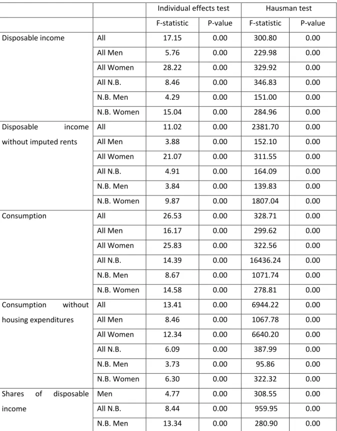
We estimated our equation for each of the variables of interest, which represents 24 estimations. As shown in Table A1 that can be found in the Appendix, in all instances, tests for fixed individual effects (which are cohort effects in our case, given by the term

∑ 𝛽_𝑐 _𝑐1_𝑗=𝑐) are positive, which justifies our choice of a fixed effects model. More

precisely, we estimate a Least Square Dummy Variable type fixed effects model. We also estimate three shares of disposable income of a subpopulation within the disposable income of the whole population and also selected a fixed effect model for those regressions.

3 Results

We now present our results by analyzing successively cohort and age effects on the various standard of living measures presented above. We first compare the effects for the whole population to those for the population without a Baccalauréat; then, we analyze separately the effects for men and women. This analysis is followed by general discussion. Period effects are not discussed here because they are not directly related to the research question of this article. All estimates are available upon request.

3.1 Standard of Living across Cohorts

For cohorts, the results are given by the estimates of the 𝛽𝑐 of the econometric model,

expressed as a deviation from a reference cohort, the one born in 1946. In the figures, the grey lines delimit the confidence interval at the 5% level.

(16)

14

Figures 3 and 4 represent the disposable income and the private consumption for the whole population, as functions of the birth date when we control for age and period effects. Those estimates are similar to those presented by d’Albis and Badji (2017), except that we consider here individualized data rather than household data controlled for the size of the household. Disposable income by date of birth (Figure 3) displays two major periods. For the cohorts born before the Second World War, income significantly increased across generations: from the 1926 cohort to the 1946 cohort it increased by 50.9%. Conversely, for post-war generations, the increase is much less pronounced and, for most cohorts, there has not been any significant change. When we exclude the imputed rents, the overall pattern is similar, although the increase is a bit less pronounced (see Figure A1 in the Appendix). For instance, from the 1926 cohort to the 1946 cohort disposable income without imputed rents rose by 43.1%. The stagnation in disposable income reveals in particular that the baby-boom cohorts do not appear to have had higher living standards than those who followed them (d’Albis and Badji 2017).

Figure 3 about here

As mentioned in d’Albis and Badji (2017), the picture is different when the private consumption is used as an indicator of the standard of living (Figure 2). The plateau that started in 1946 last till 1961, date at which cohorts started to enjoy a significant increase in consumption. The consumption of individuals of cohort 1966 is 23.3% higher than that of those who were born 20 years before while the consumption of individuals of cohort 1976 is 37.9% higher than that of those who were born in 1956. As for disposable income, the increase across generations is lowered if housing expenses are excluded (see Figure A2 in the Appendix).

(17)

15

When we restrict to the population without a Baccalauréat, the evolution of the standards of living across generations is rather different. Disposable income (Figure 5) increased first and then decreased, revealing that cohorts who were born between 1943 and 1950 enjoyed a larger disposable income that those who were born before and after them. For instance individuals without a Baccalauréat born in 1946 enjoyed a disposable income that is 26.7% larger than the one of those who were born in 1926 and 7.4% larger than the one of those who were born in 1966. When we exclude the imputed rents, the “favored” cohorts are those born between 1939 and 1950 and the shape of the curve is more symmetric, with the figures of the latter example being respectively 17.9% and 10.6% (see Figure A3 in the Appendix). As a consequence, the share of the disposable income of individuals without a Baccalauréat within the disposable income of the whole population has continuously declined over generations (Figure 6). The decline reaches 13.1% between cohort 1926 and cohort 1946 and 26.8% between cohort 1926 and cohort 1966. These figures illustrate the generational relative downgrading of the less qualified.

Figure 5 about here

Figure 6 about here

Figure 5 suggested that the less educated individuals of born during and right after the Second World War had a relative generational advantage with respect to those born before and after them. This fact is nevertheless not observed anymore when we consider consumption (Figure 7). There is no significant change between cohort 1939 and cohort 1969, and starting from cohort 1970, we observe a significant increase. For instance, individual without a Baccalauréat born in 1976 enjoy a consumption that is 17.6% higher than that of those who were born in 1956. This increase nevertheless does not appear as a robust result as we do not observe it when housing expenses are excluded from consumption (see Figure A4 in the Appendix).

(18)

16

Figure 7 about here

The breakdown by sex of disposable income reveals diverging trends. The population of men (Figure 8) has seen a much flatter variation in disposable income than the population as a whole. The rise for the pre-war cohorts is less marked and there is no further relative improvement for the 1970s cohorts compared with the 1946 cohort. As a consequence, the share of the disposable income of men within the disposable income of the whole population has generally declined over generations (Figure 9). The decrease being significant for cohorts born during the Second World War and those born after 1970.

Figure 8 about here

Figure 9 about here

The analysis is totally different with the population of women (Figure 10), who enjoyed a considerable increase in standard of living. For example, between the women of the 1926 cohort and those of the 1946 cohort, disposable income rose by 118.1%, and from the 1946 to 1966 cohorts by 23.9%. Furthermore, all the cohorts born after 1961 have a significantly higher income than the 1946 cohort. When excluding imputed rents we observe few differences as the magnitude of the increase is similar (see Figures A5 and A6 in the Appendix). Since consumption is by assumption equally shared within adults of the households, the breakdown by sex of consumption does not bring any further information than those presented in Figure 4.

(19)

17

The differential evolution of the disposable income across generation when decomposed by sex can be easily explained by the large increase in labor market participation of women over the past century. For instance, according to the French national statistical institute INSEE, the employment rate of women aged 25-49 currently reaches 75% whereas it was only 40% in 1950. Differences by sex also strongly modify the evolution of disposable income across generations of persons without a Baccalauréat. The picture presented in Figure 5 is indeed completely different when men and women are studied separately. For men (Figure 11), we observe no significant differences during a long time interval that starts with cohort 1918 and ends with cohort 1950. After that, the decline is rather strong. Men without a Baccalauréat who were born in 1976 have a disposable income that is 24.2% lower than those who were born in 1946. The decline of the share of the disposable income of men without a Baccalauréat within the disposable income of the whole population is tremendous over generations (Figure 12). The decline reaches 25.7% between cohort 1926 and cohort 1946 and 39.1% between cohort 1926 and cohort 1966.

Figure 11 about here

For women without a Baccalauréat (Figure 13), the situation is different as we see that disposable income is stable across all cohorts born after the Second World War. The comparison of Figures 11 and 13 with Figures 8 and 10 suggests that the situation of persons with tertiary education has improved since cohort 1946, both for men and women.

(20)

18 3.2 Standard of Living across Age Groups

The Figures below represent the disposable income and private consumption as functions of age, when we control for cohort and period effects. More precisely, they

represent the estimates of the 𝛼𝑖 of the econometric model. Figure 14 and 16 considers

the whole population whereas Figures 15 and 17 consider the persons without a Baccalauréat. The results are expressed as a deviation from a reference age group,

45-49 year olds7_{. As above, the grey lines delimit the confidence interval at the 5% level.}

Taking the population as a whole (Figure 14), disposable income by age increases sharply (+56%) from ages 27 to 47, then levels out until 62 and finally rises moderately (+24.9%) until age 82. One possible explanation of the rise in income after age 62 may be a composition effect similar to the one described in the literature on the missing poor in poverty statistics. Since longevity correlates with income, the proportion of low-income people declines as one moves from one higher age group to the next. However, when we consider only the persons without a Baccalauréat (Figure 15), we still observe an increase after age 62, which suggest that the missing poor hypothesis is not likely to apply here. It is actually the decomposition by sex that allows to understand the rise at late age. After age 47, disposable income tends to flatten for men, whereas it increases for women. This could be explain by the facts that women have lower labor income that are typically earned at middle-age and are more likely to survive their husband, which mechanically increase the incomes that are shared at old-age such as capital incomes. Then, the increase in disposable income after old-age 62 can be understood by a gender composition effect.

Importantly, Figures 14 and 15 reveal strong difference across education group. The increase in disposable income from ages 27 to 47 is much lower for persons without a Baccalauréat than for the population as a whole -it amounts to 27.3%- and a significant

(21)

19

decline is observed around the retirement age. The fall reaches 11.4% at age 62 compared to age 47. The general picture is that income is much flatter with age for persons without a Baccalauréat than for the rest of the population.

Those differences do not translate to consumption profiles which are remarkably similar across education groups (Figures 16 and 17). There is a significant increase in consumption over the life-cycle which reaches +26.6% from ages 27 to 47 and +40.8% from ages 47 to 67 for the whole population and, respectively +23.2% and +34.3% for the group without a Baccalauréat. It is interesting to highlight that those finding are consistent with the traditional life-cycle theory that says that income does not influence the slope of the consumption profile but its level. When housing expense are excluded, a small decline in consumption is observed after age 67 (see Figure A7 in the Appendix).

3.3 Discussion

We first remark that there can be inequality between age groups without any generation losing out. For the whole population disposable income and private consumption by age do not slope down. This implies that a person of a given age has on average a standard of living higher than or equal to that of a younger person, after controlling for cohort and period effects. But the fact that the young are less rich than

(22)

20

their current seniors does not mean that they lose out: in all our estimates, their standard of living is always higher than or equal to that of those of previous generations at the same age. D’Albis and Badji (2017) show that this is due to economic growth. Although the growth in real per capita GDP was less vigorous than during the thirty years that followed the Second World War, it was still 50% over the period considered (1979-2010). If we assume that equity between generations is ensured as long as their standard of living does not deteriorate, we may conclude that the relative position of the French cohorts born from 1901 to 1979 has been equitable.

Our breakdown of the population into men and women, however, does lead us to qualify this observation. It is clear that the rise in standard of living has been mainly enjoyed by women, whose economic position has greatly improved over this period. As an illustration, 80% of French women who were born in 1960 were part of the active population at age 40, against 65% of those born in 1940 (Afsa-Essafi and Buffeteau 2006). Conversely, men’s disposable income has varied little for all the cohorts born after the Second World War. Men’s standard of living has not got worse, but it has not improved as much as women’s. This point in no way detracts from the fact that men’s disposable income is much higher than women’s. Our observation merely reveals a catching up in women’s position with respect to men’s. As a consequence, the relative position, in terms of disposable income, of men within the population has declined across cohorts.

But the breakdown by qualification is even more instructive. We see that men without a Baccalauréat not only experience a fall in disposable income around the age at retirement but also experienced a strong generational decline after 1950. All cohorts being significantly worse than those who were born between 1918 and 1950. This decline do not appear for women without a Baccalauréat as it was probably compensated by an increase in their participation to the labor market. Three conclusions may be drawn from this. First, if we restrict to the population of men

(23)

21

without a Baccalauréat, we can observe that intergenerational equity deteriorates continuously since cohort 1950. Technical progress, globalization and public policies certainly improved the average standard of living in France since the 1970, but the non-educated men born after the Second World War did not benefitted from this improvement. Second, we never found that the baby boom generation had higher standard of living than the generations that followed. In the only case where we find a deterioration, i.e. for men without a Baccalauréat, it is more the generations that were born in the 1930s and in the 1940s that could be considered as favored. Finally, men without a Baccalauréat have clearly suffered from a large decline of their economic relative position as the share of their disposable income within the average income of the population was nearly divided by two between cohort 1926 and cohort 1966.

Our results complement recent studies that analyze the evolution of intergenerational motility. The perspective is different as it is the relative position that is measured (Goldthorpe, 2012) but is complementary to understand perceptions about intergenerational equity. Lefranc (2018) shows that intergenerational persistence of men’s income has increased since the cohorts born in the 1950s, and Alesina et al. (2018) show that the French, like other Europeans, are pessimistic about intergenerational mobility. Concerning intergenerational mobility through social classes, Vallet (2017) concludes that mobility increased for younger cohorts and that the increase was larger for women than for men while Ben-Halima et al. (2014) show that the intergenerational persistence was lower for daughter than for son.

4 Concluding Remarks

In this article, we examine the variation in standard of living between generations and between ages in France. We show that, generally speaking, standard of living did not declined from generation to generation. However, breakdown by sex does reveal that women’s position has considerably improved while men’s has stagnated for all cohorts

(24)

22

born after the Second World War. When we restrict to the population without a Baccalauréat, we show that men who were born after 1950 experienced a significant decline in disposable income with respect to those who were born between 1918 and 1950. Conversely, women without a Baccalauréat did not experienced such a decline. The tremendous diffusion of education within the French population has clearly benefited to younger cohorts -on average- and thus maintained some intergenerational equity. However, men who did not completed the secondary education, who became a minority within younger cohorts suffered from an intergenerational inequality when compared to those who had the same level of education in the previous cohorts.

This research could be improved by including other dimensions of economic welfare. An obvious one is life expectancy. It is clear that improvement here is a barometer of progress for a society and a source of well-being for individuals. This variable is therefore often included in composite indicators as, e.g., in d’Albis and Badji (2019). In the same vein, it could be also interesting to obtain mortality measures by educational attainment (Murtin et al. 2017) to see whether they soften our findings on less educated men. Case and Deaton (2015)’s works suggest it might not be the case as they revealed that in the U.S. less educated white men experienced a decline in life expectancy. Leisure is also a major constituent of well-being (Jones and Klenow 2016). The centuries-long reduction in working hours in all the developed countries (Boppart and Krusell 2016) is naturally likely to increase leisure time from one generation to the next. This would tend to support our basic conclusions that the economic welfare of generations has not declined and equity between generations has been preserved. It would, however, be useful to examine the differing changes for men and women by including time spent on domestic production. This cannot be done from the BdF survey alone, but would need to use the time use survey (named Emploi du Temps in France), which unfortunately covers a much shorter period (d’Albis et al. 2016). A further avenue for research would be income inequalities. Here it would be useful to

(25)

23

distinguish general inequalities from inequalities by age (d’Albis and Badji, 2020) and assess which mainly affect individuals’ well-being. These two further questions are on our research agenda.

References

Afsa-Essafi, C., and S. Buffeteau 2006. L’activité féminine en France : quelles évolutions récentes, quelles tendances pour l’avenir ? Economie et Statistique 398-399: 85-97. Alesina, A., S. Stantcheva and E. Teso 2018. Intergenerational mobility and preferences for redistribution. American Economic Review 108(2): 521–554.

Amossé, T. and O. Chardon 2006. Les travailleurs non qualifiés : une nouvelle classe sociale ?, Économie et Statistique 393-394: 203-229.

Arrow, K., P. Dasgupta, L. Goulder, G. Daily, P. Ehrlich, G. Heal, S. Levin, K.-G. Mäler, S. Schneider, D. Starrett and B. Walker 2004. Are we consuming too much? Journal of Economic Perspectives 18(3): 147-172.

Ben-Halima B., N. Chusseau and J. Hellier 2014. Skill premia, and intergenerational education mobility: the French case. Economics of Education Review 39: 50-64.

Boppart, T. and P. Krusell 2016. Labor supply in the past, present, and future: A balanced-growth perspective. NBER Working Paper No. 22215.

Case, A. and A. Deaton 2015. Rising morbidity and mortality in midlife among white non-Hispanic Americans in the 21st century. PNAS 112 (49): 15078-15083.

d’Albis, H. and I. Badji 2017. Intergenerational inequalities in standards of living in France. Economics and Statistics 491-492: 71-92.

d'Albis, H. and I. Badji 2019. Intergenerational inequalities in mortality-adjusted disposable income, Vienna Yearbook of Population Research 17: 37-69.

d'Albis, H. and I. Badji 2020. Les inégalités intra-générationnelles en France. PSE Working Paper N° 2020-14.

d’Albis, H., C. Bonnet, X. Chojnicki, N. El Mekkaoui, A. Greulich, J. Hubert and J. Navaux 2019. Financing the consumption of young and old in France. Population and Development Review 45 (1): 103-132.

d’Albis, H., C. Bonnet, J. Navaux, J. Pelletan, H. Toubon and F.-C. Wolff 2015. The lifecycle deficit for France, 1979-2005. Journal of the Economics of Ageing 5: 79-85. d’Albis, H., C. Bonnet, J. Navaux, J. Pelletan and F.-C. Wolff 2016. Travail rémunéré et travail domestique : une évaluation monétaire de la contribution des femmes et des hommes à l'activité économique depuis 30 ans. Revue de l'OFCE 149: 101-130.

(26)

24

Deaton, A. 1985. Panel data from time series of cross-sections. Journal of Econometrics 30: 109-126.

Deaton, A. and C. Paxson 1994. Saving, growth, and aging in Taiwan. Chicago University Press for the National Bureau of Economic Research.

Duru-Bellat, M. and A. Kieffer 2008. From the Baccalauréat to higher education in France: Shifting inequalities. Population 63(1): 119-154.

Goldthorpe, J. 2012. Understanding -and misunderstanding- social mobility in Britain: The entry of the economists, the confusion of politicians and the limits of educational policy. Barnett Papers in Social Research 2/2012.

Guillerm, M. 2017. Les méthodes de pseudo-panel et un exemple d’application aux données de patrimoine. Économie et Statistique 491-492: 119-140.

Jauneau, Y. 2009. Les employés et ouvriers non qualifiés : un niveau de vie inférieur d’un quart à la moyenne des salariés, Insee Première 1250, Juillet.

Jones, C. and P. Klenow 2016. Beyond GDP? Welfare across countries and time. American Economic Review 106(9): 2426–2457.

Lefranc, A. 2018. Intergenerational earnings persistence and economic inequality in the long run: evidence from French cohorts, 1931–75. Economica 85(340).

Le Rhun, B. and P. Pollet 2011. Diplômes et insertion professionnelle. In: France, portrait social. Insee Références. Paris.

Murtin, F., J. Mackenbach, D. Jasilionis, and M. Mira d’Ercole (2017), Inequalities in longevity by education in OECD countries: Insights from new OECD estimates, OECD Statistics Working Papers, No. 2017/02, OECD Publishing, Paris.

Stavins, R., Wagner, A. and Wagner, G. 2003. Interpreting sustainability in economic terms: dynamic efficiency plus intergenerational equity. Economics Letters 79: 339-343.

United Nations 2013. National Transfer Accounts Manual. Measuring and Analysing the Generational Economy. New York.

Vallet, L.-A. 2017. Mobilité sociale entre générations et fluidité sociale en France. Le rôle de l'éducation. Revue de l'OFCE 150(1): 27-67.

(27)

25 Appendix

Table A1. Test for fixed individual effects and Hausman test

Individual effects test Hausman test F-statistic P-value F-statistic P-value

Disposable income All 17.15 0.00 300.80 0.00

All Men 5.76 0.00 229.98 0.00 All Women 28.22 0.00 329.92 0.00 All N.B. NN.E.populat ion 8.46 0.00 346.83 0.00 N.B. Men 4.29 0.00 151.00 0.00 N.B. Women 15.04 0.00 284.96 0.00 Disposable income without imputed rents

All 11.02 0.00 2381.70 0.00 All Men 3.88 0.00 152.10 0.00 All Women 21.07 0.00 311.55 0.00 All N.B. NN.E.populat ion 4.91 0.00 164.09 0.00 N.B. Men 3.84 0.00 139.83 0.00 N.B. Women 9.87 0.00 1807.04 0.00 Consumption All 26.53 0.00 328.71 0.00 All Men 16.17 0.00 299.62 0.00 All Women 25.83 0.00 322.56 0.00 All N.B. NN.E.populat ion 14.39 0.00 16436.24 0.00 N.B. Men 8.67 0.00 1071.74 0.00 N.B. Women 14.58 0.00 278.81 0.00 Consumption without housing expenditures All 13.41 0.00 6944.22 0.00 All Men 8.46 0.00 1067.78 0.00 All Women 12.34 0.00 6640.20 0.00 All N.B. NN.E.populat ion 6.09 0.00 387.99 0.00 N.B. Men 3.73 0.00 95.86 0.00 N.B. Women 6.30 0.00 322.32 0.00 Shares of disposable income Men 4.77 0.00 308.55 0.00 All N.B. 8.44 0.00 959.95 0.00 N.B. Men 13.34 0.00 280.90 0.00

Reading note: Column 4, a P-value lower than 0.05 indicates that the test for individual effects is positive at the 5% threshold. Column 6, a P-value lower than 0.05 indicates that the fixed effects model is appropriate. N.B. stands for no Baccalauréat.

(28)

26

Additional Figures

Note: Estimates of the cohort effects in a model controlled for the age group and the period. 1946=1. Grey lines delimit the confidence interval at the 5% level.

(29)

27

(30)

28

(31)

29

Note: Estimates of the age group effects in a model controlled for the cohort and the period. 1946=1. Grey lines delimit the confidence interval at the 5% level.

(32)

30 Figures 10000 15000 20000 25000 30000 25-29 30-34 35-39 40-44 45-49 50-54 55-59 60-64 65-69 70-74 75-79 80-84

Figure 1 Disposable income as a function of age group for groups of cohorts, population without a Baccalauréat

G_1901-1904 G_1905-1909 G_1910-1914 G_1915-1919 G_1920-1924 G_1925-1929 G_1930-1934 G_1935-1939 G_1940-1944 G_1945-1949 G_1950-1954 G_1955-1959 G_1960-1964 G_1965-1969 G_1970-1974 G_1975-1979 5000 7000 9000 11000 13000 15000 17000 19000 21000 25-29 30-34 35-39 40-44 45-49 50-54 55-59 60-6 4 65-69 70-74 75-79 80-84 Figure 2 Private consumption as a function of age group for groups

of cohorts, population without a Baccalauréat

G_1901-1904 G_1905-1909 G_1910-1914 G_1915-1919 G_1920-1924 G_1925-1929 G_1930-1934 G_1935-1939 G_1940-1944 G_1945-1949 G_1950-1954 G_1955-1959 G_1960-1964 G_1965-1969 G_1970-1974 G_1975-1979

(33)

31

(34)

32

(35)

33

(36)

34

(37)

35

(38)

36

(39)

37

(40)

38