HAL Id: hal-00335046
https://hal.archives-ouvertes.fr/hal-00335046
Preprint submitted on 28 Oct 2008
HAL is a multi-disciplinary open access
archive for the deposit and dissemination of sci-entific research documents, whether they are pub-lished or not. The documents may come from teaching and research institutions in France or
L’archive ouverte pluridisciplinaire HAL, est destinée au dépôt et à la diffusion de documents scientifiques de niveau recherche, publiés ou non, émanant des établissements d’enseignement et de recherche français ou étrangers, des laboratoires
Sincere, strategic, and heuristic voting under four
election rules: An experimental study
André Blais, Jean-François Laslier, Nicolas Sauger, Karine van der Straeten
To cite this version:
André Blais, Jean-François Laslier, Nicolas Sauger, Karine van der Straeten. Sincere, strategic, and heuristic voting under four election rules: An experimental study. 2008. �hal-00335046�
SINCERE, STRATEGIC, AND HEURISTIC VOTING UNDER
FOUR ELECTION RULES: AN EXPERIMENTAL STUDY
André Blais
Jean-François Laslier
Nicolas Sauger
Karine Van der Straeten
September 2008
Cahier n°
2008-06
ECOLE POLYTECHNIQUE
CENTRE NATIONAL DE LA RECHERCHE SCIENTIFIQUE
DEPARTEMENT D'ECONOMIE
Route de Saclay
91128 PALAISEAU CEDEX
(33) 1 69333033
http://www.enseignement.polytechnique.fr/economie/
mailto:[email protected]
SINCERE, STRATEGIC, AND HEURISTIC VOTING UNDER
FOUR ELECTION RULES: AN EXPERIMENTAL STUDY
André Blais
1Jean-François Laslier
2Nicolas Sauger
3Karine Van der Straeten
4September 2008
Cahier n°
2008-06
Résumé:
Nous rendons compte d’une série d’expériences de laboratoire à propos des comportementsde vote. Dans une situation où les sujets ont des préférences unimodales nous observons que le vote à un tour et le vote à deux tours génèrent des effets significatifs de dépendance du chemin, alors que le vote par approbation élit toujours le vainqueur de Condorcet et que le vote unique transférable (système de Hare) ne l’élit jamais. A partir de l’analyse des données individuelles nous concluons que les électeurs se comportent de manière stratégique tant que les calculs stratégiques ne sont pas trop complexes, auquel cas ils se repose sur des heuristiques simples.
Abstract:
We report on laboratory experiments on voting. In a setting where subjects have single peaked preferences we find that One-round voting and Two-round voting generate significant path dependent effects, whereas Approval voting elects the Condorcet winner and Single Transferable vote (Hare system) does not. From the analysis of individual data we conclude that voters behave strategically as far as strategic computations are not too involved, in which case they rely on simple heuristics.Mots clés :
Elections, comportement de vote.Key Words :
Elections, voting behavior.Classification JEL:
D72
1
Université de Montréal, Canada
2
Ecole Polytechnique, France
3
1
Introduction
One of the most celebrated pieces of work in the field of electoral systems is due to Maurice Duverger whose comparison of electoral systems in the 1950s showed that proportional representation creates conditions favourable to foster multi-party development, while the plurality system tends to favour a two-party system (Duverger, 1951). To explain these differences, he drew a distinction be-tween mechanical and psychological effects. The mechanical effect corresponds to the transformation of votes into seats. The psychological effect can be viewed as the anticipation of the mechanical system: voters are aware that there is a threshold of representation (Lijphart 1994), and they decide not to support parties that are likely to be excluded because of the mechanical effect.
Since then, strategic voting has been considered as the central explanation of the psychological effect (Cox 1997). The assumption of rational individuals vot-ing strategically has been intensively used as a tool in formal models, on which are based most of the contemporary works on electoral systems (Taagepera 2007). In this vein, Cox (1997) and Myerson & Weber (1993) have provided models of elections using the assumption of strategic voters which yield results compatible with Duverger’s observations.
These models have had widespread appeal but are simultaneously extensively debated (Green & Shapiro 1994). In particular, the assumption of rational forward-looking voters seems to be at odd with a number of empirical studies of voters’ behaviour. Following the lines of the pessimistic view of the 19th century elitist theories, decades of survey research have concluded to the limited capacities of the electorate to behave rationally, lacking coherence of preferences (Lazarsfeld & al. 1948), lacking basic information about political facts and institutional procedures (Delli, Caprini & Keeter 1991), and lacking cognitive skills to elaborate complex strategies (for comprehensive and critical review, see Kinder 1983, Sniderman 1993 and Kuklinski & Quirk 2000). In his survey of strategic voting in the UK, Fisher (2004 : 163) posits that ”no one fulfils the abstract conception of a short-term instrumentally rational voter in real life”. Yet, Riker claims that ”the evidence renders it undeniable that a large amount of sophisticated voting occurs — mostly to the disadvantage of the third parties nationally- so that the force of Duverger’s psychological factor must be considerable” (Riker 1982: 764).
This obvious contradiction between two streams of literature needs some clarification. Testing the existence of rational strategic behaviour at the indi-vidual level with survey data is not an easy task. Indeed, rational choice theory postulates that voters cast their vote in order to maximize some expected util-ity function, given their beliefs on how other voters will behave in the election. Testing for this kind of behaviour requires measuring voters’ preferences among the various candidates as well as their beliefs on how their own vote will affect the outcome of the election.
One route to test for rational strategic behaviour from electoral survey data has been to use proxies for voters’ relevant beliefs such as the viability of can-didates (for a review, see for instance Alvarez & Nagler 2000, Blais & Bodet
2006). The basic approach is to determine whether the so-called viability of can-didates (the likelihood that they win the election) is significant when modelling individual vote choice. This is generally considered as an approximation of the core idea of the rational choice theory of voting, i.e. that voters try to maximize the utility of their vote. However, these proxies are a ’far cry’ from the concept of a pivotal vote, which is central in the rational choice model (Aldrich 1993).
To overcome these difficulties, this paper proposes to study strategic voting in the laboratory. The experiments we report differ from other laboratory exper-iments (for instance Felsenthal 1990, Forsythe & al. 1993 and 1996, Béhue & al. 2008, Morton & Rietz 2008) by important features: we have a larger number of voters participating in each election (21 or 63 voters) and a more fragmented set of options to be selected (five candidates instead of three usually). We use four different electoral systems: besides the traditional one round plurality method (labelled 1R) and two-round majority system (2R) – on which the main part of the analysis will focus – we include approval voting (AV) and the single transferable vote with Hare transfers (STV).
This experimental setting allows us to control for individual preferences for the various candidates (which are monetary induced) and for the information they have regarding the respective chances of various candidates. The aim of this paper is to test whether people, in a favourable context, are able to make the kind of computations and reasoning assumed by rational choice theory. For additional analyses of the same experiments, see Blais & al. (2007, 2008).
The rest of the paper is structured as follows. The next section describes the experiments. The following section presents the results and tests how well sincere voting, strategic voting, or the use of heuristics fare in explaining indi-vidual behaviour. Section 4 suggests a cognitive explanation to our findings and section 5 concludes. Supplementary material is provided in the Appendix.
2
The experimental protocol
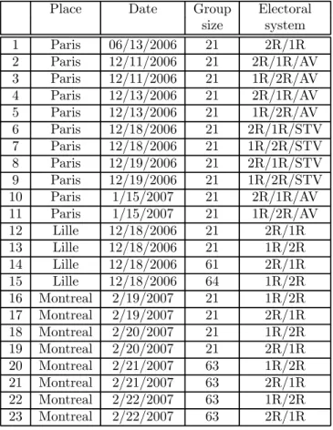
This article is based on experiments conducted in Lille, Montreal and Paris. The basic feature of these experiments has participants (students) voting in order to chose one of five possible outcomes, described as “candidates”. Voters are fully informed about the different specifications described below and the elections are performed by series of four, the results of each election being made public each time immediately. Cooperation and communication among voters are banned. The main treatment is to vary the electoral system. The two first series of elections were alternatively held under 1R and 2R. In Paris, one more series of elections was held under Single Transferable Vote or Approval Voting. The basic protocol is as follows. 21 (or sometime 63) subjects vote among five alternative candidates, located at five distinct points on a left-right axis that goes from 0 to 20: an extreme left candidate, a moderate left, a centrist, a moderate right, and an extreme right (see Figure 1).
she will earn. The monetary incentive for a subject is that the elected candidate be as close as possible to her position. Precisely, the subjects are informed that they will be paid 20 Euros (or Canadian dollars) minus the distance between the elected candidate’s position and their own assigned position. For instance (this is the example given in the instructions), a voter whose assigned position is 11 will receive 10 euros if candidate A wins, 12 if E wins, 15 if B, 17 if D, and 19 if C. In the experiment (as in real life) it is in the voter’s interest that the elected candidate be as close as possible to her own position.
The set of options and the payoff scheme are identical for all elections. In each group, 2 or 3 series of 4 elections are held successively. The four elections are held with the same voting rule. For each series the participants are assigned a randomly drawn position on the 0 to 20 axis. There are a total of 21 positions, and each participant has a different position. (For large groups three students have the same position.) The participants are informed about the distribution of positions: they know their own position, they know that each possible position is filled exactly once (or thrice in sessions with 63 students) but they do not know by whom. Voting is anonymous. After each election, ballots are counted and the results (the five candidate scores) are publicly announced.1
After the initial series of four elections, the participants are assigned new positions and the group moves to the second set of four elections, held under a different rule and, in some sessions, to a third series of four elections. The participants are informed from the beginning that one of the eight or twelve elections will be randomly drawn as the ”decisive” election, the one which will actually determine the payoffs.2.
We performed 23 such sessions in Lille, Montreal, and Paris, with a total of 734 participants. More precise information about each experiment is provided in Table 1, which indicates the order in which series of four elections were held within each session and the number of participants.3
.
3
Results
3.1
Aggregate electoral outcomes
The overall results are as follows. Table 2 shows the aggregate results for all elections and Table 3 the same results restricted to the last two elections of each series of four. The extremist candidates (A and E) are never elected. In
1For STV elections, the whole counting process occurs publicly in front of the students, eliminating the candidate with the lowest score and transferring ballots from one candidate to the other.
2This is customary in Experimental Economics; it has the advantage of keeping the subjects equally interested in all elections and of avoiding insurance effects; see Davis & Holt (1993).
3Small groups are made of 21 participants with one participant per position and large groups have 63 participants with 3 participants per position. In two large sessions held in adjacent rooms a mistake occurred so that the numbers are 61 and 64. This is of no importance for the analysis performed in the present paper, we therefore keep these data.
0 1 6 10 14 19 20
A B C D E
Figure 1: Positions of the five candidates
Place Date Group Electoral size system 1 Paris 06/13/2006 21 2R/1R 2 Paris 12/11/2006 21 2R/1R/AV 3 Paris 12/11/2006 21 1R/2R/AV 4 Paris 12/13/2006 21 2R/1R/AV 5 Paris 12/13/2006 21 1R/2R/AV 6 Paris 12/18/2006 21 2R/1R/STV 7 Paris 12/18/2006 21 1R/2R/STV 8 Paris 12/19/2006 21 2R/1R/STV 9 Paris 12/19/2006 21 1R/2R/STV 10 Paris 1/15/2007 21 2R/1R/AV 11 Paris 1/15/2007 21 1R/2R/AV 12 Lille 12/18/2006 21 2R/1R 13 Lille 12/18/2006 21 1R/2R 14 Lille 12/18/2006 61 2R/1R 15 Lille 12/18/2006 64 1R/2R 16 Montreal 2/19/2007 21 1R/2R 17 Montreal 2/19/2007 21 2R/1R 18 Montreal 2/20/2007 21 1R/2R 19 Montreal 2/20/2007 21 2R/1R 20 Montreal 2/21/2007 63 1R/2R 21 Montreal 2/21/2007 63 2R/1R 22 Montreal 2/22/2007 63 1R/2R 23 Montreal 2/22/2007 63 2R/1R
1R 2R AV STV C 49 % 54 % 79 % 0 B or D 51 % 45 % 21 % 100 % A or E 0 0 0 0
total 92 92 24 16
Table 2: Elections Won (all)
1R 2R AV STV C 52 % 50 % 100 % 0 B or D 48 % 50 % 0 100 % A or E 0 0 0 0
total 46 46 12 8
Table 3: Elections Won (last two)
1R elections candidate C (the centrist candidate, a Condorcet winner in our case) is elected in about half of the elections, and candidates B or D are elected in the remaining half (with B being elected more often than D). In 2R elections, the picture is similar but in AV elections and STV elections, it is very different. In AV elections, C is almost always elected, and in STV elections, C is never elected.
If one looks more precisely at the chronological order of the elections (from the first to the fourth for a given voting system), one finds clear path-dependence effects for 1R and 2R elections. Tables 11 and 12 in the Appendix indicate the percentage of votes (averaged over our 23 sessions) obtained by the candidates ranked first, second, third, fourth and last, and how these figures change with time. Table 13 is the same for Approval Voting, the relative score of a candidate being the percentage of voters who vote for the candidate (these percentages thus does not sum to one). Single Transferable Vote is not a score method, but one can compute the Borda scores of the candidates in the STV ballots and this is how Table 14 is computed.
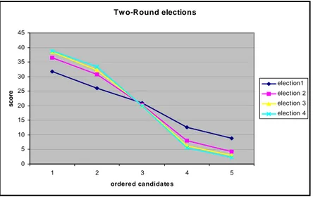
Figures ?? to 5 depict these numbers. One can see that as time goes, votes gather on two (for 1R elections) or three (for 2R elections) candidates. The three viable candidates are always the same for 2R elections (candidates B, C, D), but for 1R elections the pair of viable candidates may change among these three candidates. The pictures for AV and STV do not show any time-dependence effect.
These aggregate results show that our protocol is able to implement in the laboratory several of the theoretical issues about voting rules: with the same preference profile, voting rules designate the Condorcet winner (Approval Vot-ing), or not (STV), or designate a candidate which depends on history (1R and 2R).
The path-dependence observed at the aggregate level for 1R and 2R votes is an indication that the behaviour of a voter should be studied as a response the
One-Round elections 0 10 20 30 40 50 60 1 2 3 4 5 orde re d ca ndida te s sco re election 1 election 2 election 3 election 4
Figure 2: Ordered relative scores by date : 1R
Tw o-Round elections 0 5 10 15 20 25 30 35 40 45 1 2 3 4 5 orde re d ca ndida te s sco re election1 election 2 election 3 election 4
Figure 3: Ordered relative scores by date : 2R
Approval elections 0 10 20 30 40 50 60 70 1 2 3 4 5 orde re d ca ndida te s ap p ro val sc o re election 1 election2 election3 election4
STV elections 0 10 20 30 40 50 60 70 1 2 3 4 5 orde re d ca ndida te s B o rd a s c ore election 1 election 2 election 3 election 4
Figure 5: Ordered Borda scores by date for STV
3.2
Three models of individual behaviour
We start with an analysis of individual behaviour for 1R and 2R elections. We present and compare three theoretical models that could account for individual vote choice. Section 3.3 tests the models with the data.
Note that in a second round of a two-round election, the choice faced by voters is very simple: they have to vote for one candidate among the two run-off candidates. In particular, voting for the candidate associated with the highest monetary payoff is a dominant strategy. Therefore, the models we propose below are intended to describe behaviour in the first round of 2R elections; in the sequel, when we talk about behaviour and scores in 2R elections, unless otherwise specified, we mean behaviour and scores in the first round.
3.2.1 Sincere voting
For 1R and 2R elections, the simplest behaviour than can be postulated is “Sin-cere” voting, which means that the individual votes for the candidate whose posi-tion is closest to her own posiposi-tion. To be more specific, we introduce the following notation: there are I voters, i = 1, 2, ..., I, and 5 candidates : A, B, C, D, E. The monetary payoff received by voter i if candidate c wins the election is denoted by ui(c). In plurality one round and majority two round elections, individual i votes for a candidate v∗ such that:
ui(v∗) = max
v∈{A,B,C,D,E}ui(v).
if the voter’s position is precisely in between two adjacent candidates, which is the case of voters on the 8th and 12th position on our axis. The sincere prediction does not depend on history.
3.2.2 Strategic voting
By strategic behaviour we mean that an individual, at a given date t, chooses an action (a vote) which maximizes her expected utility given her belief about how the other voters will vote in the current election. Strategic voting is understood, in this paper, in the strict rational choice perspective (see Downs 1957, Myerson & Weber 1993).4 We assume that voters are purely instrumental and that there is no expressive voting, so that the only outcome that matters is who wins and the utility of a voter is her monetary payoff.
For each candidate v, voters evaluate the likelihood of the potential outcomes of the election (who wins the election) if they vote for candidate v, and they compute the associated expected utility. They vote for the candidate yielding the highest expected utility.
To be more specific, let us denote by pi(c, v) the subjective probability that voter i assigns to the event “candidate c wins the election”, conditional on her casting her ballot for candidate v5. Given these beliefs, if voter i votes for candidate v, she gets the expected utility
Wi(v) = X
c
pi(c, v)ui(c).
Individual i votes for a candidate v∗such that:
Wi(v∗) = max
v∈{A,B,C,D,E}Wi(v).
For example, if candidate c is perceived to be a sure winner then whatever the vote decision v of voter i is, pi(c, v) = 1 and pi(c0, v) = 0, for all c0 other that c. In such a case, voter i gets the same expected utility whoever she votes for, since candidate c will be elected no matter what she does. In that case, Wi(v) = ui(c), for all v ∈ {A, B, C, D, E}. Any vote is compatible with the strategic model in that case.
This model leaves open the question of the form of the probabilities pi(c, v), which reflect the predictions that voter i makes regarding other voters’ behav-iour, and so one has to make some specific assumptions regarding these proba-bilities. A first possibility, that we call the “rational expectation” assumption, is simply to assume that voters’ beliefs about other voters’ behavior are correct. This assumption is common in Economic Theory. It lacks realism because it
4Note that the definition of strategic voting we use here does not coincide with that which is sometimes given in the literature in political science. Indeed, this literature has traditionally opposed a sincere and a strategic (or sophisticated) voter, where a voter is said to be strategic only when she deserts her preferred option (Alvarez & Nagler 2000; Cox 1997). Such strategic voting needs not be utility maximizing..
5withP
amounts to postulate that the voter “knows” something which has not taken place yet, but it is theoretically attractive because it avoids the delicate question of the belief formation process. A second possibility, that we call the “myopic” assumption, is to assume that each voter forms her beliefs about how other voters will behave in the current election based on the results of the previous election and thinks that other voters will behave in the current election just as they did in the previous election.6 A “myopic” theory only makes prediction for the second, third, and fourth elections in each series (t = 2, 3 or 4). It does not predict how voters behave before they observe any results. On the other hand the rational expectation hypothesis makes predictions even for the first date.
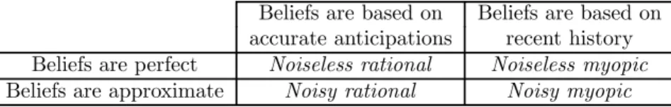
Myopic beliefs as well as rational expectations or any other kind of beliefs, can be precise or approximate. The former assumption will be labelled “noise-less” and the latter “noisy”. Under the “noisy rational expectation” the voter is supposed to know approximately the other voters’ actual vote (see table 4). Under the “noisy myopic” assumption the voter believes that the other voters’ current vote will be approximately the same as the previous vote. Noisy models draw on the refinement literature from Game Theory and consider “trembled” beliefs (Selten, 1975; see Myerson, 1991 ch. 5). We make the hypothesis that the individual believes that the votes of the other participants will be very close to, but not exactly equal to, what they are supposed to be. Precisely,each voter considers that with a small probability ε, exactly one other voter is going to make a mistake, by deviating from her postulated action and voting with an equal probability for any of the remaining four candidates.
Note that with the noiseless assumption, the only case where a voter is piv-otal – and thus where she is not indifferent – is when the vote gap between the first two candidates is strictly less that 2 (either 1 or 0). The introduction of a small noise increases the chances that any voter becomes pivotal: under this assumption, a voter can be pivotal when the vote gap between the first two candidates in strictly less that 4 (and not 2 as under the noiseless assump-tion). When there is a unique best response for the voter under the noiseless assumption, this action is still the unique best response when there are very small “trembles” in other voters’ votes (ε small); but when the best response under the noiseless assumption is not unique, considering small trembles may break ties among the candidates in this set.
This noisy assumption seems more reasonable from a cognitive point of view; and is also preferable from a methodological point of view because it more often yields unique predictions.7
The Appendix describes precisely how to derive the pi(c, v) probabilities under the various assumptions and for the different voting rules. We performed
6All this applies to 1R-elections and to the first rounf of 2R-elections. Now, in 2-round elections, these pi(c, v)involve both beliefs as to how voters will behave at the second round (if any), and beliefs as to how voters will behave at the first round. We assume that each voter anticipates that at the second round (if any), each voter will vote for the candidate closest to her position, and will toss a coin if the two run-off candidates are equally close to her position. 7If a voter knows precisely how the other voters will vote, she will generally conclude that her own vote does not matter.
Beliefs are based on Beliefs are based on accurate anticipations recent history Beliefs are perfect Noiseless rational Noiseless myopic Beliefs are approximate Noisy rational Noisy myopic
Table 4: Beliefs specifications
analyses based on these four different assumptions. Analyses under the rational and the myopic expectations turn out to yield very similar results (see the Appendix). For ease of exposition, we report in the main text only the findings based on the noisy rational expectation assumption.
3.2.3 Heuristics
The third set of models tested in this paper is based on the idea of bounded rationality. Over the past two decades, several authors have discussed the con-clusion of limited competence of citizens from the observation of widespread political ignorance. As Sniderman et al. (1991), Popkin (1991), and Lupia and McCubbins (1998) have argued, it is possible for people to reason about politics without a large amount of knowledge thanks to heuristics. Heuristics, in this context, can be defined as ‘judgemental shortcuts, efficient ways to organize and simplify political choice, efficient in the double sense of requiring relatively little information to execute, and yielding dependable answers even to complex problems of choice’ (Sniderman et al. 1991: 19). We focus in this paper on a specific type of heuristics, linked to the structure of competition rather than on policies or issues (in the same perspective, see Patty 2007, Lago 2008, Laslier 2008).
Building on the literature on electoral systems, the heuristics we are inter-ested in define the viability of candidates. Rather than engaging in complex computations as assumed in the strategic voting model, voters rely on a prin-ciple of choice in a restricted menu. The general idea of the heuristics is that voters vote sincerely in the set of viable candidates. The viability of candidates is defined by a general rule, specific to each electoral system. From the rule given by Gary Cox (1997) that there are M + 1 viable candidates, M being the district magnitude, we test two heuristics. The “Top-Two heuristics” posits that voters choose the candidate they feel closer to among the candidates who obtained the two highest scores in the previous election. This rule should apply to 1R electoral systems. The “Top-Three heuristics” posits that voters choose the candidate they feel closer to among the top three candidates. This heuris-tics should apply to 2R electoral systems since the first round of 2R system can be viewed as having a magnitude of two, two candidates moving to the second round.
1R Sincere Strategic Top-Two Top-Three % correct predictions 49.4% 72.5% 72.0% 69.1% (testable predictions) 1985 1358 2083 2000
Table 5: Model performance for 1R elections
3.3
Test of the models
The general approach is to compare the predictions of the theoretical models with the observations. It consists in computing for each theory the predictions in terms of individual voting behaviour and to determine how many times these predictions coincide with observations (Hildebrand & al. 1977).
The main developments are dedicated to 1R and 2R elections. AV and STV will help to strengthen our general argument. Our main conclusion is that the rational theory of strategic voting performs surprisingly well but only in simple contexts. As soon as strictly rational strategies become more complex or less intuitive, people apparently use shortcuts and their behaviour is better captured by a heuristics framework
3.3.1 Results for One-Round elections
Table 5 indicates the percentage of correct predictions for the various theories. We use the noisy rational version of Strategic voting. The percentages are computed only on the cases where the theory makes a unique and testable prediction. We consider only the data relative to dates 2 to 4. Not taking the first date into account allows to compare the myopic and rational expectations assumptions (this is done in the Appendix); moreover we already know that learning is taking place, so the initial elections are hardy comparable with the others. Detailed statistics by date , details of the test that we performed, with a complete description of the theories, are presented in the Appendix in subsection 7.2.
Sincere voting is clearly not as good as the other theories in that case. It makes a unique prediction except if the voter’s position is precisely in between two adjacent candidates (case of voters on the 8th and 12th position of our axis). If we restrict attention to the cases of unique predictions, we observe that the sincere voting theory is performing rather poorly: The theory explains about 49% of the votes on average for elections 2 to 4, and this figure is decreasing with time: in the first election of the series of four it is 69% but in the last elections it is 45%. (See Table 15 and more details on the sincere theory in 1R elections in subsection 7.2.1).
The Strategic and Top-Two theories perform very well and indeed they are almost identical in that case, both in principle and in practice; the difference is that the strategic theory (in the version we use) does not provide a unique recommendation when the first-ranked candidate is two or more votes ahead of the second-ranked one. Surprisingly the Top-Three theory works quite well too. To explain this fact, note that the Top-Two and Top-Three theories differ
2R Sincere Strategic Top-Two Top-Three % correct predictions 58.1% 59.2 % 61.3% 72.7% (testable predictions) 1989 375 2080 1987
Table 6: Model performance for 2R elections
essentially when the voter’s preferred candidate among candidates B, C and D is ranked third. This is for instance the case for an extreme-right voter when D is ranked third after B and C. In such a case the voter may desert her sincere choice E but still not move to support C against B, like the Strategic and Top-Two theories would command, and instead move to support the moderate candidate D.
The figures are given here using the “Rational expectations” version of the theories. The findings are the same using the “myopic” versions (see the Ap-pendix). The analysis date by date confirms that Sincere voting is decreasing with time, and Strategic or Top-Two voting are increasing.
We conclude that, in 1R elections, our subjects essentially behave in accor-dance with the Strategic paradigm and the Top-Two heuristics. Sincere voting is clearly the least satisfactory model. Both the heuristics and the strategic models perform much better. The former has the advantage of yielding more unique predictions. The latter has the virtue of being grounded on more solid theoretical foundations. This seems to us a particularly important considera-tion, and so we are inclined to conclude that the rational strategic model is the most interesting in this case.
Remark on the number of unique predictions in the strategic models. Note that a way to obtain more unique predictions in the strategic model would be to increase the level of noise. Under the noiseless assumption, the anticipations are extremely precise. Under the noisy assumption as postulated here, each voter considers that with a small probability ε, exactly one other voter is going to make a mistake, by deviating from her postulated action and voting with an equal probability for any of the remaining four candidates. A further refinement would be to assume that with a smaller probability (say ε2), exactly two other votersare going to make a mistake, by deviating from their postulated action and voting with an equal probability for any of the remaining four candidates. In the approval strategic section, this is actually the route we follow, by assuming that any number of mistakes is possible (with decreasing probability), see subsection 3.3.3.
3.3.2 Results for Two-Round elections
Table 6 compares models for the first round of 2R elections. Again, Sincere voting is not satisfactory, but, contrary to the previous case, the strategic the-ory does not perform much better. The best predictor is here the Top-Three heuristics. Its predictive power is high (72.7% on average) and increasing with time (74.7% for fourth elections, see the Appendix).
The conclusion here is quite clear as to the relative success of the theories: the simple Top-Three heuristics beats both the sincere and the strategic theories.
3.3.3 Results for Approval Voting
Sincerity under Approval voting The definition of “sincere” voting un-der AV is that a voting ballot is sincere if and only if there do not exist two candidates a and b such that the voter strictly prefers a to b and nevertheless approves of b and not of a. With this definition we can count, in our data at each election and for each voter the number of pairs (a, b) of candidates such as a violation of sincere voting is observed. Such violation of sincere voting is very rare in our data: 78 observed pairs out of 5040, that is 1.5%.
This definition of sincere voting leaves one degree of freedom to the voter since it does not specify at which level, given her own ranking of the candidates, the voter should place her threshold of approbation. With 5 candidates most voters have 6 sincere ballots (including the “full” and the”empty” ballots).
Consequently the notion of “Sincere voting” does not provide a predictive theory in the case of Approval Voting and thus cannot be compared with other theories.
Strategic behaviour under Approval voting In order to make strategic predictions at the individual level, we use a slitghtly different scheme from the one we used for 1R and 2R elections. The reason is that, with this voting rule, the voter is asked to provide a vote (positive or negative) about all candidates, including those who have virtually no chance of winning according to the voter’s own belief. In 1R and 2R elections, under the noisy assumption as we defined it, a voter assumed that with a small probability, exactly one voter would make a mistake (from the refernce situation). The probability put on higher "orders of mistakes" (two voters make a mistake, three voters make a mistake, ...) was zero. With AV, this model does not produce a unique prediction as to how a voter should fill her ballot. Instead, we use in that case a model with much higher levels of uncertainty, by putting some positive probabilities on all possible events (although the probability is exponentially decreasing with the number of mistakes). We do not compute with computers the probabilities of the various outcomes in that case, and instead borrow from the literature on strategic voting under AV (see Laslier 20088). It turns out that the maximization of expected utility under such a belief is easy to perform and often provides a unique strategic recommendation (Laslier 2008). This prediction can be described as follows. The voter focuses on the candidate who is obtaining the largest number of votes, say a1. All other candidates are evaluated with respect to this leading candidate a1: the voter approves all candidates she prefers to a1and disapproves all candidates
8who considers the following voter belief: The voter anticipates the result of the election (the number of approvals that he or she thinks a candidate is to receive, not including the individual’s own approval) and she tells herself : “if my vote is to break a tie, that will be between two (and only two) candidates and that might occur because any other voter, with respect to any candidate, can independently make a mistake with some small probability ε.
Approval =1 Approval=0 total Prediction=1 590 157 747 Prediction=0 69 982 1051
total 659 1139 1798
Table 7: AV: 88% of approbations predicted by the“strategic" model
Approval =1 Approval=0 total Prediction=1 619 119 738 Prediction=0 121 995 1116
total 740 1114 1854
Table 8: AV: 87% of approbations predicted by the“best two" model
she finds worse than a1. The leading candidate is evaluated by comparison with the second-ranked candidate (the “main challenger”): the voter approves the leading candidate if and only if she prefers this candidate to the main challenger. The voter therefore places her “Approval threshold” around the main candidate, either just above or just below.
Details of this “leading candidate” theory are provided in the Appendix. It produces 1798 unique predictions out of 21 ∗ 6 ∗ 5 ∗ 3 = 1890 votes. The unique predictions are correct in 590 +982 = 1572 cases out of 1798, that is 87%, as one can see in Table 7. The Table distinguishes these predictions, right or wrong, according to the observed vote. The theory tends to slightly overestimate the number of approved candidates.
Heuristics for Approval voting The strategic model described above leads to behavioral recommendations which are very simple: Place your “Approval threshold” around the main candidate, either just above or just below. There-fore, we suspect that any simple heuristic based on the viability of candidates (as are the top-two or top-three heuristics used for 1R and 2R elections) would yield similar recommendations.9
Rather, we present here the test for a heuristic that, contrary to those de-velopped sor far, does not rely on the viability of the candidates. We also tested for the heuristics model which simply predicts that the voter approves her two preferred candidates. Table 8 indicates the predictions of this theory relative to the last three periods of each series (for the sake of comparison). The number of observations is 1890 votes and we have 1854 unique predictions.10 On the set of possible predictions this simple theory predicts 619 + 995 = 1615 votes, that is 87% .
9Such an adaptation of the "top-two" heuristic to AV would be the following. Consider the two candidates that get the highest number of votes in the reference election (not taking into account the voter’s own ballot). The voter should approve of the candidate she likes best among these two candidates, as well as all the candidates that she ranks higher.
Of course this nice result (87% of explained votes) is due to the fact that we calibrated the theory to an observed variable: the average number of approval per ballot is about 2, so it is quite clear that the “Best two” heuristics works better here than the “Best one” or the “Best three” heuristics.
Conclusion on Approval voting Under approval voting, the Sincere voting paradigm does not provide clear predictions. Votes are well predicted by the Strategic theory and by a “Best two” heuristics. On the face of the present experiment, we cannot distinguish between these. But notice that, in other circumstances, the average number of approbations per ballot might be notably different. For instance Laslier and Van der Straeten 2008, in a quite different setting, report an average number of approval of 3.15 out of 16 candidates. In such a case it is clear that the “Best two” heuristics will be invalidated. We thus conclude in favour of the strategic theory for Approval voting.
3.3.4 Results for Single Transferable Vote (Hare method)
Under this voting rule, voters have many different ballots at their disposal since they are asked to submit a complete ranking of candidates. For 5 candidates, there are 121 possible ballots. We look for violations of sincere voting by counting the number of pairs of candidates (a, b) such that a voter strictly prefers a to b but nevertheless ranks b higher than a in her ballot. There are 5972 such pairs, of which only 600, that is 10%, violate sincerity. We therefore find that sincerity is satisfied at 90% for this voting rule.
This simple observation enables us to understand what has been observed in our STV elections. Since voters vote (approximately) sincerely, given our preference profile the two extremes candidates – who receive the votes of the extreme voters – are always eliminated first. Then (for the third round of the vote transfers), the two moderate candidates have more votes than the centrist candidate, who has received no transferred votes. Therefore the centrist candidate, despite being a Condorcet winner, is always eliminated at the third round.
Sincere voting is clearly a satisfactory theory here. Note that the published literature on this voting rule does not propose, to our knowledge, a practical solution to the question of individual strategic voting under STV with five can-didates. We (so far) did not attempt to compute the rational recommendation at the individual level for this voting rule as we did for other rules. These computations would be similar, but much more complex than those for 2R elec-tions. In particular, these computations would entail specifying each voter’s beliefs regarding how all other voters filed their ballots (in order to be able to proceed to the successive eliminations of candidates). The assumption of ratio-nal anticipations in that case seems hard to take in. and the myopic version would entail specifying voters’ beliefs about the part of the abllots that they did not learn during the previous counting of ballots (although the whole counting process occurs in front of the subjects, only some (little) part of the relevant
1R 2R Sincere 49% 58% Strategic 72% 59% Top-Two 72% 61% Top-Three 69% 73%
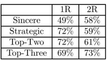
Table 9: Comparing models on unique predictions, all last three elections
information to compute an optimal response is learned through it). Therefore, we did not attempt to test the strategic models for this voting rule.
4
A cognitive explanation
Table 9 compares models and voting rules by presenting the explanatory power of various theories for 1R and 2R elections
As already mentioned, the first result is that sincere voting theory is not able to explain much of what we observed in 1R and 2R elections. In 1R elections the “explanatory power” of this theory is on average close to 50% and is decreasing with time. In 2R elections, it is 58%, also decreasing. Strategic theory explains well the data in 1R elections (72%, increasing) but not in 2R elections (59%). This is the puzzle we will now try to solve: Why does rational behaviour explains the data in 1R elections but not in 2R elections?
One point is common to strategic behaviour in both cases: one should not vote for a candidate who has no chance to play a role in the election. In our data set, it is clear that, in all elections, the two extreme candidates had no chance. Based on this idea, it is easy to find a theory which explains well individual behaviour in our 2R elections. Suppose that the voters vote for their (sincerely) preferred candidates among the three candidates who obtain the most votes in the last election. This “Top-Three” theory has a predictive power of 73% (out of 1987) in 2R elections. This point is perfectly in line with the remark that precisely three candidates are viable in 2R elections. The “Top-Two” theory (preferred candidate among the two candidates who obtain the most votes in the last election) does not do well for 2R elections (61%, decreasing) but is a very reasonable theory for 1R elections (72%, increasing).
In order to understand better why individual behaviour is deviating from strict rationality in 2R elections, we now restrict our attention to the cases when sincere voting is unique but is not “rational”. Strategic voting (in the noisy rational version) makes a unique prediction and Sincere voting makes another, different, one. These are the cases where the individual is facing a dilemma. Table 10 reports how she is resolving this dilemma, depending on her position; the numbers in this Table indicates the percentage of dilemmas which are resolved by a sincere (and thus irrational) choice.
One can see that in 2R elections moderate voters whose strategic recommen-dation (following our noisy model) would contradict their sincere vote prefer (at
1R 2R Extremists (0-3, 17-20) 86/439 = 20% 11/43 = 26% Moderates (4-7, 13-16) 68/147 = 46% 74/91 = 81% Centrists (8-12) 28/56 = 50% 6/13 = 46%
Table 10: Sincere choice in front of a dilemma
81%) to follow the sincere recommendation. These individuals are for most of them located at positions 7 and 13. Consider for instance the voter at position 7. She earns 19, 17 or 13 when candidates B, C or D is elected. According to our model, she anticipates that she will earn 17 if C goes to the second round because C will then be elected. If the second round is B against D, she has the expected utility: (19 + 13)/2 = 16. Such a voter should rationaly vote for C because promoting C to the second round is the best way to avoid the election of the bad candidate D. It seems that this kind of reasoning leading to “inverse strategic voting” (Blais 2004) is not followed by our subjects. On the other hand extremists voters in 1R election massively follow the strategic recommendation rather than the sincere one, under both voting rules.
This suggests that our subjects voted strategically when the strategic rec-ommendation is simply to desert a candidate who is behaving poorly, but they do not vote strategically when strategic reasoning asks for a more sophisticated and counter-intuititve calculus. This conclusion is in line with our findings about Approval voting. Voting strategically under Approval voting is not difficult for the voter, and it never contradicts a basic notion of “sincerity”: the voter es-sentially defines “good” and “bad” candidates by comparison with the most serious candidate. On the contrary, the logical computations required for vot-ing strategically under STV are extremely complexe. We observed that voters voted sincerely under this voting rule. This is in line with the actual prac-tice of similar systems in countries where parties offer to take away from the voter the burden of strategic reasoning by recommending a whole ranking of the candidates (see Farrell & McAllister 2006).
5
Conclusion
Reporting on a laboratory experiment on voting under different electoral sys-tems, this article has compared three models to explain voting decisions at the individual level. The first model is based on the notion of sincere voting, the second relies on the rational choice theory, and the third on heuristics. We have shown that these different approaches perform differently under different voting rules.
We define Sincere voting in the usual way, which raises no problem in the laboratory since individual preferences are controlled. Sincere voting can then be meaningfully tested for most voting rules, except for Approval voting.
Strategic voting is defined following the rational choice paradigm as the max-imization of expected utility, given a utility function and a subjective probability
distribution (“belief”) on the possible consequences of actions. Utilities are con-trolled as monetary payoffs. Beliefs are endogenous to the history of elections, and we showed that two reasonable forms of beliefs (“rational anticipations” and “myopic anticipations”) yield the same conclusions.
The heuristics considered in this paper are to vote for the preferred candi-date among the two (“Top-Two”) or three (“Top-Three”) candicandi-dates who are perceived as the most likely to win. These heuristics rely on the same beliefs as Strategic voting and we have again shown that rational and myopic anticipations yield the same conclusions.
For One-round elections, the sincere voting model behaves very poorly be-cause it fails to predict the desertion of un-viable candidates. Strategic voting is a good model in that case and is essentially identical (in principle and in practice) to the Top-Two heuristics.
For Two-round elections, the best theory is the Top-Three heuristics. We observe that un-viable candidates are also deserted (which invalidates Sincere voting); but when strategic computations lead to paradoxical conclusions such as voting for a disliked candidate in order to increase its chances to be present in the second round, these recommendations are not followed. This is inconsistent with Strategic voting as we defined it and thus explains the limited perforance of this models in the context of two round elections.
We therefore conclude that voters tend to vote strategically as far as the strategic reasoning is not too complex, in which case they rely on simple heuris-tics.
Our observations on Approval voting and Single Transferable vote confirm this hypothesis. In the case of Approval voting, strategic voting is simple and produces no paradoxical conclusions; we observe that our subjects voted strate-gically under this system. On the contrary, voting stratestrate-gically under STV is a mathematical puzzle; and we observed that voters voted sincerely under STV.
This article has departed from classical approaches to strategic voting. Rather than estimating the role of different factors in the econometric “vote equation”, we proposed to compute directly predictions of individual behaviours accord-ing to several theories (sincere votaccord-ing, strategic votaccord-ing and votaccord-ing accordaccord-ing to behavioural heuristics). The main results of this study underline the good per-formance of the strategic voting theory to explain the behaviour of our subjects in One-round plurality elections or Approval voting. Support for this theory is however weaker in more complex settings, such as run-off elections and STV, for which other theories outperform strategic voting theory in explaining individual decisions.11
The amount of “unsincere” voting observed in our experiments appears to be higher than that reported in studies based on surveys (see, especially, the summary table provided in Alvarez and Nagler 2000), though such comparisons are difficult to make because sincere and strategic choices are not defined the same way. This is not strictly due to the limitations in size of our groups of
1 1If one was to define “strategic” voting as voting non-sincerely then our results about Two-round elections would validate the strategic hypothesis, but we choose a more precise definition of strategic voting.
students, though this experiment has obviously taken the form of voting in committees. The variation from 21 to 63 subjects has not lead to significant change in our results (see also Blais et al. 2008).
Why this amount of unsincere voting is so high on our setup? We would suggest three possibilities. First the amount of unsincere voting may depend on the number of candidates. We had five candidates in our setup, while most survey-based studies are restricted to three parties. Further work is needed, both experimental and survey-based, to determine how the propensity to vote sincerely is affected by the number of candidates. Secondly, our findings show that the amount of sincere voting declines over time, which indicates that some of our participants learn that they may be better off voting unsincerely. This raises the question whether voters in the real life, where an election is not followed immediately by another election, still manage to learn over time. Third, in our setup participants had a clear rank order of preferences among the five candidates. Blais (2002) has speculated that perhaps many voters have a clear preference for one candidate or party and are rather indifferent among the other options, which weakens any incentive to think strategically. We need better survey evidence on that matter, and also other experiments in which some voters are placed in such contexts. Anyway, the most likely answer is that this experiment has little external validity in terms of estimation of level of sincere or unsincere voting precisely because it has focussed on the line of reasoning people follow in forming their vote choice.
Our main concern in this study has not been to estimate the amount of sincere, strategic, or heuristic voting. The purpose has rather been to see how three different models could explain vote choice under different voting rules. We have shown that the sincere model works better for a very complex voting system where strategic computations appear to be insurmountable, that the strategic model performs well in simple systems, and that the heuristic perspective is most relevant in situations of moderate complexity. These findings make eminent sense. And it is a virtue of the experimental design to allow us to compare vote choice under different voting rules.
6
References
ALDRICH, J. H. (1993) Rational choice and turnout. American Journal of Political Science, 37, 246-278.
ALVAREZ, R. M. & NAGLER, J. (2000) A new approach for modelling strategic voting in multiparty elections. British Journal of Political Science, 30, 57-75. BEHUE, V., P. FAVARDIN and D. LEPELLEY (2008) “La manipulation stratégique des règles de vote: une étude expérimentale” forthcoming in Recherches Economiques de Louvain.
BLAIS, A. (2002). “Why Is There So Little Strategic Voting in Canadian Plu-rality Rule Elections?” Political Studies 50: 445-454.
BLAIS, A. (2004). “Y a-t-il un vote stratégique en France?” IN CAUTRES, B. and MAYER, N. (Ed.) Le nouveau désordre electoral: les leçons du 21 avril 2002. Paris, Presses de la Fondation nationale des sciences politiques.
BLAIS, A.and BODET (2006) “Measuring the propensity to vote strategically in a single-member district plurality system” mimeo, university of Montréal. BLAIS, A., J-F. LASLIER, A. LAURENT, N. SAUGER and K. VAN DER STRAETEN, 2007, ”0ne round versus two round elections: an experimental study”, French Politics 5: 278-286.
BLAIS, A., S. LABBE-ST-VINCENT, J-F. LASLIER, N. SAUGER and K. VAN DER STRAETEN, 2008, ”Vote choice in one round and two round elec-tions”, mimeo.
COX, G. W. (1997) Making Votes Count : Strategic Coordination in the World’s Electoral Systems, Cambridge, Cambridge University Press.
DAVIS, D. D. & C. A. HOLT (1993) Experimental Economics, Princeton: Prince-ton University Press.
DELLI CAPRINI, M. X. & S. KEETER (1991) Stability and change in the US public’s knowledge of politics. Public Opinion Quarterly, 55, 581-612.
DOWNS, A. (1957) An Economic Theory of Democracy, New York, Harper and Row.
DUVERGER, M. (1951) Les partis politiques, Paris, Armand Colin.
FARRELL, D., & I. MCALLISTER (2006) The Australian Electoral System: Origins, Variations, and Consequences, Sydney, University of New South Wales Press.
FELSENTHAL, D. S. (1990) Topics in Social Choice. Sophisticated Voting, Efficacy, and Proportional Representation, New York, Praeger.
FISHER, S. (2004) Definition and measurement of tactical voting: the role of rational choice. British Journal of Political Science, 34, 152-66.
FORSYTHE, R., T. A. RIETZ, R. MYERSON and R. J. WEBER (1993) ”An Experiment on Coordination in Multicandidate Elections: the Importance of Polls and Election Histories,” Social Choice and Welfare 10: 223-247
FORSYTHE, R., T. A. RIETZ, R. MYERSON and R. J. WEBER (1996) “An Experimental Study of Voting Rules and Polls in Three-Way Elections” Inter-national Journal of Game Theory, 25: 355-383.
GREEN, D. P. & SHAPIRO, I. (1994) Pathologies of Rational Choice Theory : A Critique of Applications in Political Science, New Haven, Yale University Press.
HILDEBRAND, D. K., LAING, J. D. & ROSENTHAL, H. (1977) Prediction Analysis of Cross Classifications, New York, Wiley.
KINDER, D. R. (1983) “Diversity and complexity in American public opin-ion”. In FINIFTER, A. (Ed.) Political Science: the State of the Discipline. Washington, American Political Science Association.
KUKLINSKI, J.H., and QUIRK, P.J. (2000). “Reconsidering the Rational Pub-lic: Cognition, Heuristics, and Mass Opinion.” IN LUPIA, A., MCCUBBINS, M.D., and POPKIN, S.L.(Ed.) Elements of Reason: Cognition, Choice, and the Bounds of Rationality. Cambridge, Cambridge University Press.
LAGO, I. (2008) “Rational expectations or heuristics? Strategic voting in pro-portional representation systems”. Party Politics, 14, 31-49.
LASLIER, J.-F. (2008) “The Leader Rule: A model of strategic approval voting in a large electorate” forthcoming, Journal of Theoretical Politics.
LASLIER, J.-F. and K. VAN DER STRAETEN (2008) “A live experiment on Approval Voting” Experimental Economics 11:97-105.
LAZARSFELD, P., BERELSON, B. R. & GAUDET, H. (1948) The People’s Choice: How the voter makes up his mind in a presidential campaign, New York, Columbia University Press.
LIJPHART, A. (1994) Electoral Systems and Party Systems: A Study of Twenty-Seven Democracies, 1945-1990, Oxford, Oxford University Press.
LUPIA, A., AND MCCUBBINS, M. (1998). The Democratic Dilemma: Can Citizens Learn What They Need to Know? New York, Cambridge University Press.
MORTON, R. B.. and RIETZ, T. A. (2008) “Majority requirements and mi-nority representation” mimeo.
MYERSON, R. B. (1991) Game Theory: Analysis of Conflict. Harvard Univer-sity Press.
MYERSON, R. B. & WEBER, R. J. (1993) “A theory of voting equilibria”. American Political Science Review, 87, 102-114.
PATTY, J. (2007) “Incommensurability and issue voting” Journal of Theoretical Politics 19: 115-131.
POPKIN, S. L. (1991) The Reasoning Voter: Communication and persuasion in presidential campaigns, Chicago, Chicago University Press.
RIKER, W. H. (1982) Liberalism Against Populism: A confrontation between the theory of democracy and the theory of social choice, San Francisco, W.H. Freeman.
SELTEN, R. (1975) “Re-examination of the perfectness concept for equilibrium points in exten,sive games” International Journal of Game Theory 4: 25-55. SNIDERMAN, P. M. (1993) “The new look in public opinion research”. IN FINIFTER, A. (Ed.) Political Science: the State of the Discipline II. Washing-ton, American Political Science Association.
SNIDERMAN, P. M., TETLOCK, P. E. & BRODY, R. A. (1991) Reasoning and Choice: Explorations in political psychology, Cambridge, Cambridge University Press.
TAAGEPERA, R. (2007) “Electoral systems”. IN BOIX, C. & STOKES, S. C. (Eds.) The Oxford Handbook of Comparative Politics. Oxford, Oxford Univer-sity Press.
candidates dates % 1st 2nd 3rd 4th 5th t = 1 32.8 27.3 20.8 11.8 7.2 t = 2 39.2 33.5 18.2 6.2 2.9 t = 3 44.3 36.0 14.3 4.4 0.8 t = 4 51.3 36.0 8.7 3.3 0.5
Table 11: Ordered relative scores, by date : 1R
candidates dates % 1st 2nd 3rd 4th 5th t = 1 31.7 26.0 21.0 12.6 8.8 t = 2 36.5 30.8 20.3 8.0 4.3 t = 3 38.5 32.2 20.2 6.2 3.0 t = 4 38.8 33.4 19.9 5.5 2.3
Table 12: Ordered relative scores, by date : 2R
7
Appendix
7.1
Time-dependency for agregate results
Tables 11 to 14 show the evolution of the ordered candidate scores for the four electoral systems, they correspond to Figures ?? to ?? in the main text .
7.2
One Round elections
7.2.1 Sincere voting theory (1R)
Description. Individuals vote for any candidate that yields the highest payoff if elected. Individual i votes for a candidate v∗ such that:
ui(v∗) = max
v∈{A,B,C,D,E}ui(v).
Predictions. Sincere Voting is independent of time. For all voters except those in position 8 and 12, this theory makes a unique prediction. Voters in
po-candidates dates % 1st 2nd 3rd 4th 5th t = 1 56.3 50.0 42.9 30.2 25.4 t = 2 57.1 47.6 43.7 28.6 23.0 t = 3 53.2 46.0 43.7 28.6 21.4 t = 4 59.5 46.0 42.1 26.2 22.2
candidates dates % 1st 2nd 3rd 4th 5th t = 1 56.3 50.0 42.9 30.2 25.4 t = 2 57.1 47.6 43.7 28.6 23.0 t = 3 53.2 46.0 43.7 28.6 21.4 t = 4 59.5 46.0 42.1 26.2 22.2
Table 14: Ordered Borda scores, by date : STV
t = 1 t = 2 t = 3 t = 4 total 1R 455662 = 69% 363662 = 55% 322661= 49% 296662 = 45% 14362647 = 54% 2R 489657 = 74% 406663 = 61% 385663= 58% 363663 = 55% 16432646 = 62%
Table 15: Sincere Voting for single-name elections
sition 8 are indifferent between B and C and voters in position 12 are indifferent between D and C.
Test. When we restrict ourselves to unique testable predictions12, this theory correctly predicts behaviour on 54% of the observations, but this figure hides an important time-dependency: the predictive quality of the theory is decreasing from 69% at the first election to 45% at the fourth one; see Table 15. which also compares with 2R elections. 13
7.2.2 Strategic models in one-round elections
Strategic behaviour under the no-noise (ε = 0) assumption (1R)
Description with Rational Anticipations. Assumption 1 (No noise, Rational Anticipations) : Each individual has a correct anticipation of the vote of the other individuals at the current election.
In that case,the subjective probabilities pi(c, v) are constructed as follows. Consider voter i at t-th election in a series (t = 1, 2, 3, 4). Voter i correctly anticipates the scores of the candidates in election t, net of her own vote. The subjective probabilities pi(c, v) are then easily derived. Let us denote by L the set of first-ranked candidates (the leading candidates), and by F the set of closest followers (considering only other voters’ votes). (i) If the follower(s) is (are) at least two votes away from the leading candidate(s), if voter i votes for (one of) the leading candigate(s), this candidate is elected with probability 1, if she votes for any other candidate, there is a tie between the leading candidates
1 2A prediction, even unique, is not testable in the case of a missing or spoiled ballot, which explains why the denominators in Table15 are not exactly the same. We should have 664 sincere predictions at each date, that is 2656 on the whole. There are very few missing or spoiled ballots (about .3%).
1 3To compare with the other Tables, the figures in the main text are computed for dates 2 to 4. That is 981/1985 = 49.4% for 1R and 1154/1989 = 58.0% for 2R.
1 2 3 4 5 total 823 18 30 343 1722 2936 28.0% 0.6% 1.0% 11.7% 58.7% 100%
Table 16: Multiple Predictions, ² = 0, 1R
(if there is only one leading candidate, he is elected for sure).14 (ii) If now the two sets of candidates L and F are exactly one vote away: if voter i votes for (one of) the leading candigate(s), this candidate is elected for sure; if she votes for (one of) the followers, there is a tie between this candidate and the leading candidates; if she votes for any other candidate, there is a tie between the leading candidates.15
Predictions. Under these assumptions regarding the pi(c, v) , we com-pute (using Mathematica software) for each election (starting from the second election in each session) and for each individual, her expected utility when she votes for candidate v ∈ {A, B, C, D, E}: that isPcpi(c, v)ui(c). We then take the maximum of these five values. If this maximum is reached for only one candidate, we say that for this voter at that time, the theory makes a unique prediction regarding how she should vote. If this maximum is reached for sev-eral candidates, the theory only predicts a subset (which might be the whole set) of candidates from which the voter should choose.
Consider for example a situation where, at the current election, one candi-date is expected to be a clear leader (he is alone ahead by a three votes margin or more). This candidate is expected to win for sure and no voter is pivotal. Thus all voters are indifferent between voting for any candidate. All ballots yields the same expected payoff for them, that is the monetary payoff each gets when that leading candidate is elected.
The table 16 gives the statistics regarding the number of candidates in this subset. These figures are obtained considering all four dates 1 to 4. The total number of observations is thus 734 × 4 = 2936.
In 823 cases, the theory makes a unique prediction as to vote behaviour and in 1722 cases any observation is compatible with the theory. Note that in 343 cases, it recommends not to vote for a given candidate.
1 4 Formally,
if v ∈ L: pi(v, v) = 1and pi(c, v) = 1for all c 6= v,
if v /∈ L: pi(c, v) = |L|1 if c ∈ L and pi(c, v) = 0for all c /∈ L, where |L| is the number of leading candidates.
1 5 Formally,
if v ∈ L: pi(v, v) = 1and pi(c, v) = 1for all c 6= v,
if v ∈ F : pi(c, v) = |L|+11 if c ∈ L ∪ {v} and pi(c, v) = 0for all c /∈ L ∪ {v}, if v /∈ L ∪ F : pi(c, v) =|L|1 if c ∈ L and pi(c, v) = 0for all c /∈ L.
(1R) t = 2 t = 3 t = 4 total Testable predictions 212 269 157 638 Correct predictions 149 = 70% 211 = 78% 139 = 89% 499 = 78%
Table 17: Testing strategic noiseless theory, rational anticipations, 1R
(1R) t = 2 t = 3 t = 4 total Testable predictions 181 212 270 663 Correct predictions 125 = 69% 167 = 79% 235 = 87% 527 = 79%
Table 18: Testing strategic noiseless theory, myopic anticipations, 1R
Test We restrict attention to the last three elections of each series. This theory makes unique predictions in 638 testable cases, of which 499 are correct, that is 78%.
Comparison with the myopic version. The “Myopic” version of the theory is very similar to the “Rational Anticipations” but the assumption 1 becomes :
Assumption 1bis (No noise, Myopic Anticipations) : Each individual assumes that during the current election, all voters but herself will vote exactly as they did in the previous election.
Comparing Tables 17 and 18 one can see that the qualitative conclusions to be drawn from these two variants will be identical.
Strategic behaviour under the small-noise (ε > 0) assumption (1R)
Description with Rational Anticipation. Assumption 2 (Small noise, Rational Anticipations) : Each individual belief is a small perturbation of the actual votes of the other individuals at the current election.
More precisely, consider voter i. Her belief is a probability distribution over the set of possible behaviour of the other voters. With probability ε (small), one voter exactly (taken at random among the I − 1 remaing voters) makes a mistake and does not vote for the intended candidate, but instead, with equal probability votes for one of the other four candidates.
Note that the number of unique predictions is higher in the noisy case than in the noiseless case. Indeed, we take ε extremely close to zero, so that each time the strategic theory yields a unique prediction under the noiseless assump-tion, the noisy theory yields the same unique prediction. To see why the noisy assumptions yields unique predictions in many other cases, consider for exam-ple voter i in the following situtation: in the current election, not taking into account his own vote, she is sure that a candidate will be alone ahead leading
1 2 3 4 5 total 1977 28 12 153 766 2936 67.3% 1.0% 0.4% 5.2% 26.1% 100%
Table 19: Multiple Predictions, ² > 0, 1R
by two votes (the rational noiseless assumption). With this noiseless assump-tion, voter i is not pivotal, whoever she votes for, this leading candidate wins with probability 1, and therefore voter i is indifferent between voting for any candidates. Now, with the noisy assumption, this voter also assigns a smlall but positive probability to other events. If ε is small enough, the most likely event is still by far the situation where this leading candidate is still two votes ahead. But there is now a small probability that voter i might be pivotal. Indeed, for example, if one of the voters who is supposed to vote for the leading candidate rather votes for the second-ranked candidate, then these two candidates will receive exactly the same number of votes, and in this event, voter i becomes pivotal.
If a vote v is strictly better than another vote v0 for ε = 0, it will remain so for ε > 0 provided that the probability ε is small enough. Consequently the theory ε > 0 is a refinement of the theory ε = 0, just like trembling-hand perfection is a refinement of Nash equilibrium.
Predictions. In that case, the probabilities pi(c, v) are harder to write down in an explicit way. But they can easily be computed using Mathematica software. Under these assumptions regarding the pi(c, v), we compute (using Mathematica software) for each election (starting from the second election in each session) and each individual, his expected utility when he votes for candi-date v ∈ {A, B, C, D, E}: that is,Pcpi(c, v)ui(c). We then take the maximum of these five values. If this maximum is reached for only one candidate, we say that for this voter at that time, the theory makes a unique prediction regarding how he should vote. If this maximum is reached for several candidates, the theory only predicts a subset of candidates from which the voter should choose. The table 19 gives the statistics regarding the number of candidates in this subset. These figures are obtained considering all four dates 1 to 4. The total number of observations is thus 734 × 4 = 2936.
In 1977 cases, that is 67.3%, the theory makes a unique prediction as to vote behaviour. This is much more than what we had with the no-noise assumption (28.0%).
Test. We restrict attention to the last three elections of each series. This theory makes unique predictions in 1358 testable cases, of which 984 are correct, that is 72.5%.
Comparison with the myopic version. The “Myopic” version of the theory is very similar to the “Rational Anticipations” but the assumption 2
(1R) t = 2 t = 3 t = 4 total Testable predictions 583 512 263 1358 Correct predictions 374 = 64.2% 382 = 74.6% 228 = 86.7% 984 = 72.5%
Table 20: Testing strategic noisy theory, rational anticipations, 1R
(1R) t = 2 t = 3 t = 4 total Testable predictions 610 582 513 1705 Correct predictions 390 = 63.9% 431 = 74.1% 426 = 83.0% 1247 = 73.1%
Table 21: Testing strategic noisy theory, myopic anticipations, 1R
becomes :
Assumption 2bis (Small noise, Myopic Anticipations) : Each individual belief is a small perturbation of the actual the vote of the other individuals at the previous election. More precisely, we use exactly the same model for the perturbation as before, but the reference scores are now the scores obtained at the previous election not the current one.
Comparing Tables 20 and 21 one can see that the qualitative conclusions to be drawn from these two variants will be identical.
7.2.3 “Top two” theory (1R)
Description. Individuals vote for their preferred candidate among the two candidates that get the highest two numbers of votes in the current (“Rational Anticipation” version) or the previous (“Myopic” version) election.
More precisely, consider individual i and denote by s−i(c) is the score (num-ber of votes) that candidate c obtains in the reference election (the current or the previous one), taking into account the ballots of all voters but i. Voter i can rank candidates according to those scores. If two candidates at least rank in the first place, then individual i votes for his preferred candidate among them. If only one candidate rank first, the individual votes for his preferred candidate among the set consituted of this first-ranked canked candidate and candidate(s) getting the second highest score.
Predictions. This theory makes unique predictions in almost all cases, double predictions may occur when a voter’s position is just between two candidates.
Test. This theory correctly predicts behaviour on approximately 70% of the observations. Tables 22 and 23 show the time-evolution, and show again that the two versions “rational anticipations” and “myopic anticipations” are similar.