HAL Id: hal-01053745
https://hal.archives-ouvertes.fr/hal-01053745
Submitted on 1 Aug 2014HAL is a multi-disciplinary open access
archive for the deposit and dissemination of sci-entific research documents, whether they are pub-lished or not. The documents may come from teaching and research institutions in France or abroad, or from public or private research centers.
L’archive ouverte pluridisciplinaire HAL, est destinée au dépôt et à la diffusion de documents scientifiques de niveau recherche, publiés ou non, émanant des établissements d’enseignement et de recherche français ou étrangers, des laboratoires publics ou privés.
using a fictitious domain approach
Isabelle Ramière, Michel Belliard, Philippe Angot
To cite this version:
Isabelle Ramière, Michel Belliard, Philippe Angot. On the simulation of Nuclear Power Plant Com-ponents using a fictitious domain approach. NURETH-11, Oct 2005, Avignon, France. paper: 193. �hal-01053745�
ON THE SIMULATION OF NUCLEAR POWER PLANT
COMPONENTS USING A FICTITIOUS DOMAIN APPROACH
Isabelle Ramièrea b 1, Michel Belliarda, Philippe Angotb
aCEA-Cadarache, DEN/DTN/SMTM/LMTR, 13108 St-Paul-Lez-Durance, France
Phone: +33 (0) 4 42 25 71 46, Fax: +33 (0) 4 42 25 77 67 E-Mail:[isabelle.ramiere,michel.belliard]@cea.fr
bLATP-CMI, Technopôle de Château-Gombert, 13453 Marseille cedex 13, France
E-Mail: [ramiere,angot]@cmi.univ-mrs.fr ABSTRACT
This paper describes the first step of the introduction of fictitious domain methods (FDM) in the simu-lation of nuclear component fields. We consider the resolution of a diffusion problem ✁ div
✂
˜a✄✆☎ ˜u✝✟✞ ˜f,
in a physical domain ˜✠
, with different kinds of boundary conditions (B.C.). The shape of this domain is of the Steam Generator’s type. The aim of this work is to present several ways to impose B.C. on an immersed interface, without modifying locally the numerical scheme and without using Lagrange multi-pliers. The numerical resolution is implemented using either a finite element or a finite volume method. Error estimates are performed in order to evaluate the capability of this method. A comparison with unstructured mesh methods is also presented.
KEYWORDS
Fictitious domain method, Immersed interface, Neptune, Steam Generator. 1 INTRODUCTION
Within the framework of the federal program NEPTUNE launched by the CEA and EDF concerning the
industrial simulation of two-phase flows in the nuclear power plant components as steam generators
(SG) or cores, we propose investigations of new numerical methods based on structured meshes. The advantages of numerical methods for partial differential equations (PDE) involving structured meshes are well known : easy implementation for fast solvers (based for instance on finite volume methods with structured grids) and for multi-scale methods (Angot et al. , 1993), good convergence properties, easy simulation of moving boundaries (for example moving obstacles in a flow, fluid/structure interaction...) ... However their main drawback is the difficulty to take into account boundaries or obstacles in complex industrial situations. As a fact, numerical methods involving unstructured meshes are classical in the industrial software world.
1.1 Fictitious domain method
Since a few years, fictitious domain methods (FDM)(Saul’ev, 1963. (in Russian), Marchuk, 1982 (1rst ed. 1975)) have been arising for Computational Fluid Dynamic (Khadra et al. , 2000). In this approach, the initial computation domain ˜✠
(called physical domain) is immersed in a geometrical bigger and simpler other one
✠
, called fictitious domain (see Figure 1).
The spatial discretization is now performed in the fictitious domain ✠
, independently of the shape of the physical domain ˜
✠
. The physical domain and the computational one are uncoupled. Numerical methods involving structured meshes can be computed. Consequently, in
✠
, the resolution of the new
1
Ω Ω Fictitious domain Physical domainΩ~ e External domain
Figure 1: Example of a physical domain ˜ immersed in a fi ctitious domain
equation will be fast and simple.
The main difficulty lies in the choice of the PDE solved in the fictitious domain
✠
and in the numerical scheme used for the resolution. These two choices have to be coupled in order to take into account the conditions on the initial boundary ✁ ˜
✠
. Therefore the restriction of the solution on the physical domain is expected to be the initial problem’s one.
Numerically, there are mainly three approaches to deal with the boundary conditions located on the immersed boundary:
✂
“Thin” interface approaches : the physical boundary is approximated without being enlarged in the normal direction. The physical boundary and the approximated one lie in the same✄
n space.
For example, in this group, we can find truncated domains methods (McCorquodale et al. , 2001, Ye et al. , 1999), immersed interface methods (I.I.M.) (Leveque & Li, 1994), as well as an adapted Galerkin method proposed by Latché (submitted (october 2003)).
✂
“Spread” interface approaches : the support of the approximated interface is larger than the physi-cal one. The approximated interface has one dimension more than the physiphysi-cal one. For example, the boundary can be estimated as the set of the elements of discretization crossed by itself. In particular, this kind of approach is used in the interface boundary methods (I.B.M.) (Cortez & Minion, 2000).
✂
Lagrange multipliers : in FDM using Lagrange multipliers (Glowinski & Kuznetsov, 1998), the initial B.C. are imposed weakly as side constraints. This approach doesn’t use a continuous ap-proximated boundary but only needs discretization points lying on the initial boundary.
Moreover, penalization methods (Angot, 1999, Khadra et al. , 2000) have proved their efficiency to impose values on an immersed interface or to solve suitable equations in different domains.
In this paper, one is interested in a spread interface approach computed with a usual F.E. Scheme as well as a thin interface approach computed using a F.V. Scheme with flux and solution jumps (Angot, 2003) are exposed.
A lot of papers are dedicated to embedded Dirichlet or Neumann B.C., e.g. (Saul’ev, 1963. (in Russian), Marchuk, 1982 (1rst ed. 1975), Glowinski & Kuznetsov, 1998, Glowinski et al. , 1996, Leveque & Li, 1994) and the reference herein... Only a few studies are devoted to other embedded Fourier B.C. (Kopˇcenov, 1974. (in Russian), Marchuk, 1982 (1rst ed. 1975), Angot, 1999). The fictitious domain approaches presented here deal with Dirichlet, Robin or Neumann B.C. on an immersed interface without requiring neither the modification of the numerical scheme near the
immersed interface nor the use of Lagrange multipliers. Since the fictitious problem ✂✁
✝ isn’t
a saddle-point problem, the inf-sup condition must not be verified (Glowinski & Kuznetsov, 1998). Moreover, only one discretization grid is used (the structured regular mesh over the fictitious domain).
1.2 Presentation of the test problem
For sake of simplicity we choose to focus on 2D problems, but the formulations can be extended to 3D problems without more difficulty. We study the resolution of a diffusion problem in the unit disk ˜
✠
. For symmetry reasons, we can solve this problem only on a quarter of this disk.
Let us consider the following model problem: ˜ ✠✄✂ ✄ 2 open-bounded domain For ˜a ☎ ✂ L✆ ✂ ˜ ✠ ✝ ✝ 2✝ 2 and ˜f ☎ L 2✂ ˜ ✠
✝, find ˜u defined on
˜ ✠ such that ✞ ✟✡✠ ✁ div ✂ ˜a✄✆☎ ˜u✝ ✞ ˜f in ˜ ✠ ✂ ˜a✄✆☎ ˜u✝ ✄n✞ 0 on ˜ ☛ B.C. on☞ (1) where B.C. represents : ✂
a Dirichlet condition : ˜u✞ uD,
uD ☎ H 1✌2 ✂ ☞ ✝ z x 1 1 Ω Γ ~ ~ Σ ✂
a Robin (or Fourier) condition : ✁
✂ ˜a✄✆☎ ˜u✝ ✄n✞✎✍ R ✂ ˜u✁ uR✝✑✏ gR, ✍ R ☎ L ✆ ✂ ☞ ✝✓✒✔✍ R ✕ 0 ✖ uRand gR ☎ L 2✂ ☞ ✝
(with n the outward normal unit vector on the circle)
Remark: a Neumann condition, ✁
✂
˜a✄✆☎ ˜u✝ ✄n ✞ g, is considerate as a particular Robin condition
where✍ R
✗ 0 and gR ✗ g.
Moreover, the symmetric tensor of diffusion ˜a✗
✂
˜aij✝1
✘ i j✘ 2verifies the classical ellipticity assumption:
✙ ˜a0 ✚ 0 ✖✜✛✣✢✤☎ ✄ 2 ✖ ˜a ✂ x✝ ✄✡✢ ✄✡✢ ✕ ˜a0✥ ✢ ✥ 2a ✄e✄ in ˜ ✠ ✂ A1✝ where ✥ ✄
✥ is the Euclidean norm in
✄
2.
In that case, classical variational techniques (Dautray & Lions, 1988) prove the existence and the uniqueness of the solution ˜u ☎ H
1✂
˜
✠
✝ of this problem.
For sake of simplicity, we suppose here that uD and uR are constant. The non constant cases can be
treated without more difficulty (e.g. with cell-centered approximation of these variables). In a fictitious domain approach, the quarter disk is immersed in the unit square
✠ ✞✧✦0✖ 1★✪✩✫✦0✖ 1★. z x 1 1 Ω Γ Γ ∼ ∼ Σ Ω e Ωe
In the next section, we present in detail the numerical methods implemented on the fictitious domain
✠
. For each method, the equation solved on the fictitious domain is introduced. We expose several ways to impose the different B.C. on an immersed interface for a diffusion problem. Then, in Section 3, the accuracy of this fictitious domain approach will be illustrated with numerical results. To conclude, future works and perspectives are pointed out.
2 NUMERICAL METHODS 2.1 Finite Element (F.E.) Method
2.1.1 Numerical scheme
The F.E. numerical resolution is implemented using a 1 F.E. Scheme, where k stands for the space
of polynomials of degree of each variable less than or equal to k. For example, 1 ✞ span✁ 1✖ x✖ y✖ xy✂
in✄
2. The
1discretization nodes are located on the vertex of the discrete elements.
A “spread” interface approach has been chosen. The set of the discretization elements K crossed by the immersed interface
☞ forms the approximated interface✄ h ☎ .
Discretization of the fictitious domain✠ :✠˜ h,✄ h ☎ and ✠ e h
In comparison with the initial formulation, the equation solved in
✠
hcontains additional terms that
impose the initial B.C.. Given a rectangular mesh✆ h of
✠
, the problem solved on the discrete fictitious domain
✠
hhas the following generic form :
Find uh ☎ Vh ✞✝✁ vh ☎ C 0✂✠ ✝✓✖ vh ✥K ☎✞ 1✛ K ☎✟✆ h✂ ✂ H1 ✂ ✠ ✝ such that ✞ ✟ ✠ ✁ div ✂ a✄✆☎ uh✝✑✏ b ✂ uh ✁ uE✝ ✞ f ✏ ✠ in ✠ h ✂ a✄✆☎ uh✝ ✄n ✞ 0 on ˜ ☛ suitable B.C. for uh on ☛ e (2) where a ☎ ✂ L✆ ✂ ✠ h✝ ✝ 2✝ 2 (symmetric tensor), f✖✡✠ ✖uE ☎ L 2✂ ✠ h✝, and b ☎ ✂ L✆ ✂ ✠ h✝ ✝ such that: a✥ ˜ ☛ h ✞ ˜a ✥˜ ☛ h ✖ f ✥ ˜ ☛ h ✞ ˜f ✥˜ ☛ h
a satisfies the assumption (A1) in
✠
hand b the following one:
✙ b0 ✕ 0 ✖ b ✂ x✝ ✕ b0 a ✄e✄ in ✠ h (A2)
Here too, if the B.C. on the exterior fictitious boundary
☛
e are not uniquely Neumann conditions,
variational techniques (Dautray & Lions, 1988) allow to conclude that the approximated solution uh of
the problem (2) exists and is unique.
The additional terms b✖uE and ✠ enable to take into consideration the immersed boundary (Khadra et al. , 2000, Angot et al. , 1999). We expect thus that uh✥ ˜
☛
h
✞ ˜u ✥˜
☛
h. For each kind of boundary conditions lying on the immersed boundary☞ , different possibilities to impose these conditions without modifying the numerical scheme and without using local unknowns are presented in Section 2.1.2. 2.1.2 Treatment of the initial B.C.
✂
Dirichlet case:
The Dirichlet B.C. are treated by penalization (Angot et al. , 1999). Setting b ✞
1
☞
(where 0 ✌✎✍✏✌✑✌ 1 is called penalty coefficient) and uE ✞ uD enables to impose uh ✞ uD. It’s the L2-penalty. When the coefficient a is also equal to 1☞
(a✞
1
☞
Id), we obtain the H1-penalty. The
other coefficients of the equation (2) are arbitrary extensions in
✠
on ˜
✠
(Ramière et al. , in preparation).
In Section 3, we will compare the penalization of the spread interface to the penalization of the
exterior domain.
Concerning the B.C. on☛
e, for a penalization of the spread interface, the Dirichlet B.C. uh ✞ uD
must only be imposed on the nodes lying on✄ h ☎✁
☛
e. The B.C. on the rest of
☛
ehave no influence
on the solution obtained in the physical domain. To penalize the exterior domain, the B.C. on the whole exterior boundary☛
emust be Dirichlet B.C. uh✥✂ e ✞ uD.
✂
Robin case:
We consider the continuous transmission problem between ˜✠
and ✠
e. The addition of the two
weak formulations of the two diffusion subproblems defined on respectively ˜
✠ and ✠ eleads to the following problem : Find u ☎ H 1✂ ✠ ✝ such that✛ v ☎ H 1✂ ✠ ✝ ✄ ☛ a✄✆☎ u✄✆☎ v dV ✞ ✄ ☛ f v dV✁✏✌ ★★ ✂ a✄✆☎ u✝ ✄n✦✦ ☎✆☎ ☎ ✖ v ✚ (3) where ✝ ★★ ✂ a✄✆☎ u✝ ✄n✦✦ ☎ ✞ ✂ a✄✆☎ u✝ ✄n ✥✟✞☎ ✁ ✂ a✄✆☎ u✝ ✄n ✥✡✠☎
☎ ☎ is a measure carried by the hypersurface ☞ ✖ ☎ ☎☞☛ v ✌ ✌ ☎ ☎ ✖ v ✚ ✞✎✍ ☎ v ✥ ☎ dS
In the distribution sense, we obtain the following equation:
✁ div ✂ a✄✆☎ u✝ ✞ f ✁ ★★ ✂ a✄✆☎ u✝ ✄n✦✦☎ ☎ ☎ (4)
The jump of flux across☞ can be interpreted as a source term carried by☞ .
In our case, we want
✁ ✂ a✄✆☎ u✝ ✄n ✥✡✠☎ ✞✄✍ R ✂ u✁ uR✝✑✏ gR and ✁ ✂ a✄✆☎ u✝ ✄n ✥✟✞☎ ✞ 0 so that ★★ ✂ a✄✆☎ u✝ ✄n✦✦ ☎ ✞✄✍ R ✂ u✁ uR✝✑✏ gR On ✠ , then we have: ✁ div ✂ a✄✆☎ u✝ ✞ f ✁ ★✡✍ R ✂ u✁ uR✝✑✏ gR✦ ☎ ☎ (5)
However, with a structured mesh on
✠
, the support of ☞ is not exactly defined. We introduce a characteristic parameter✏ in order to approximate the measure
☎ ☎ supported by
☞ by mollifiers
(Brezis, 2000) on the spread interface✄ h ☎ .
The principle is the following:
✄ ☎ ✁ ✍ R ✂ u ✁ uR✝ ✏ gR✂ v dS ✞ ✄✒✑ h✓✔ ✍ R ✂ u✁ uR✝ ✏ gR ✏ v dV ✛ v ☎ Vh (6)
The equation solved on
✠ his: ✁ div ✂ a✄✆☎ uh✝ ✞ f ✁ ★ ✍ R ✏ ✂ uh ✁ uR✝ ✏ gR ✏ ✦ ☎ ✑ h✓✔ (7) where☎ ✑ h✓✔
is a measure carried by the spread interface✄ h ☎ .
With the equation (7), the parameter of the generic formulation (2) can be easily set. Only the B.C. of the nodes lying on✄ h
☎✕
☛
ehas an effect on the solution obtained in the physical
domain. These B.C. must be homogeneous Neumann B.C. in order to have an external flux equal to zero. However the B.C. on the whole boundary☛
ecan’t be homogeneous Neumann B.C. since
the problem solved on ✠
becomes in this case bad-posed. The solution obtained on the fictitious domain won’t be unique. So the B.C. on☛
eare separated into two B.C.:
✝ ✂ a✄✆☎ uh✝ ✄n ✞ 0 on✄ h ☎ ☛ e uh ✞ uext otherwise
where uextis unspecified.
The parameter ✏ can be estimated by several ways (Ramière et al. , in preparation). We present
some of them in Section 3. If h is the discretization step, Angot (1989) showed that✏ is in
✂
h✝.
2.1.3 Local adaptive mesh refinement (A.M.R.)
Using a spread interface approach, A.M.R. techniques are necessary to improve the accuracy of the solution near the immersed interface and by the way on the whole physical domain. Most of these techniques are derived from multi-grid methods (Hackbusch, 1985).
A Local Defect Correction (L.D.C.) method (Hackbusch, 1984) is performed. This method is a multi-grid method with a defect restriction in the ascent step. The local refinement zone is composed by all the elements of the spread interface✄ h
☎ and their neighbors. This choice enables to correct the values
of all the nodes located on the spread interface. As a consequence, the immersed B.C. are imposed more precisely. As the solution of an elliptic problem strictly depends on the B.C., we expect an improvement of the solution on the physical domain.
2.2 Finite Volume (F.V.) Method
2.2.1 Numerical scheme
The F.V. numerical resolution is performed using a model of fracture with flux and solution jumps (Angot, 2003).
Given an “admissible” finite volume mesh✆ hof
✠
(Angot, 2003), with cell-centered discretization nodes, let S be the family of edges or sides ✁ of the “control volumes” K
✂
✆ h. Let n✂ be the unit
normal vector on ✁ oriented from K to the exterior. For a function✄ in L
2✂ ✠ ✝ , let✄ ✞ and ✄ ✠ be the
traces of✄ on each side of✁ . We define the arithmetic mean of traces of✄ as✄
✥ ✂ ✞ ✂ ✄ ✞ ✏☎✄ ✠ ✝✝✆ 2
and the jump of traces of✄ on✁ , oriented by n ✂ , as ★★✄ ✦✦ ✂ ✞ ✂ ✄ ✞ ✁✞✄ ✠
✝ . Then, the following fracture
conditions lie on each side✁
✂ S : ★★ ✂ a✄✆☎ uh✝ ✄ n ✂ ✦✦ ✂ ✞ ✍ ✂ ✂ uh✥ ✂ ✁ U ✂ ✝ ✁ h ✂ (8) ✂ a✄✆☎ uh✝ ✄ n✂ ✥ ✂ ✞ ✟ ✂ ★★uh✦✦✂ ✁ g✂ (9)
where the transfer coefficients ✍ ✂ ✖✝✟ ✂ satisfy the following ellipticity assumptions:
✍✠✂ ✖✝✟✡✂ ☎ L ✆ ✂ ✁ ✝✓✒ ✙ ✟ 0 ✕ 0 ✍☛✂ ✂ x✝✓✖✝✟✡✂ ✂ x✝ ✕ ✟ 0on✁
and g✂ ✖ h✂ and U✂ are given in L
2✂ ✁ ✝ .
The finite volume scheme built on✆ hdoesn’t introduce unknowns located on the side of the volume
con-trol. Indeed, the equations (8) and (9) enable to express these unknowns according to the cell-centered ones.
This F.V. scheme is based on a “thin” interface approach.
In this F.V. approximation, we suppose that the thin approximated interface ☞ h lies on sides of
con-trol volumes crossing the physical interface ☞ . n
☎
h denotes the outward unit normal vector of ☞ h
(n☎
h✄n
☎
✚ 0). Equations (8) and (9) enable to impose the immersed B.C. on ☞ h.
The problem solved on
✠
(a) Exterior thin interface
(b) Interior thin interface
(c) “Cut” thin in-terface
Figure 3: Examples of thin approximated interface
2.2.2 Treatment of the initial B.C.
We are interesting in the B.C. lying on the immersed approximated interface☞ h. On the sides ✁ ✆☎ ☞ h, ✁ ☎ S ✁ ✂ ˜ ☛✄✂ ☛ e✝, we set: ✍ ✂ ✞ h✂ ✞ g✂ ✞ 0 and ✟ ✂ ✌✆☎ ✂✞✝ ✂ ✞ 1 ✟ ✂ ✞ 0✖ fracture resistance✝ (10)
Remark: Locally, on the physical domain ˜✠
h and on the exterior domain
✠
e h, we get a F.V. scheme
without jump of flux and without jump of the solution as in (Eymard et al. , 2000). We focus on the transfer coefficients lying on✁ ☎ ☞ h
✁ ✂ ˜ ☛✄✂ ☛ e✝ . ✂ Dirichlet case:
We present two manners to deal with a Dirichlet condition.
The first one consists in penalizing the exterior domain at uD. To impose uD on the
in-terior side of the approximated interface ☞ h (side located in the physical domain), we set ✟ ✂ ✞ 1 ☞ ✛ ✁ ☎ ☞ h ✁ ✂ ˜ ☛✟✂ ☛
e✝. The other transfer coefficients are equal to zero.
In the second approach, uDis imposed directly by surface penalization on the approximated
in-terface☞ husing the jump equations (8) and (9). We set✟ ✂ ✞
1☞ in order to have u✞ ✞ u ✠ on ✁ and then u✥ ✂ ✞ u ✞ ✞ u ✠ ✞ u ✥
✂ . In this case, penalizing also ✍ ✂ ✞
1
☞
while setting U✂ ✞ uDinduces
u✂ ✞ uD ✛ ✁ ☎ ☞ h
✁ ✂
˜
☛✠✂ ☛
e✝. The exterior domain has no influence on the solution obtained in
the physical domain.
In these two approaches, the B.C. on☞ h
☛
eare the only one of interest : uh✥
☎ h✡ ✂ e ✞ uD. ✂ Robin case: We want that ✁ ✂ a✄✆☎ uh✝ ✄n ☎ h✥✠☎ h ✞✄✍ R ✂ u✥ ☎ h ✁ uR✝✑✏ gR, where u ✥ ☎ h ✞ u ✠ ✥ ☎ h.
There are many ways to deal with the transfer coefficients in order to impose a Robin B.C. on☞ h
(there is five coefficients for 2 equations). One of particular interest is the one without control on
the exterior domain. In this case, we eliminate ✁
✂ a✄✆☎ uh✝ ✄n ☎ h✥✞☎ h and u✞ ✥ ☎ h in the equations (8) and (9): ✛ ✁ ☎ ☞ h ✁ ✂ ˜ ☛✟✂ ☛ e✝ ✍ ✂ ✞ 2✍ R✖ ✟ ✂ ✞ ✍ R 2 ✖ u✂ ✞ uR✖ h✂ 2 ✁ sg ✂ n☎ h✄n✂ ✝ g✂ ✞ gR ✂ e✄g✄ h✂ ✞ ✁ 2gRand g✂ ✞ 0✝
As in the spread interface approach, a characteristic parameter✏ is required to respect the
equal-ity between the flux carried by the approximated interface and the flux carried by the physical immersed interface.
The B.C. on☛
e
✁
☞ h are free (without effect on the solution on the physical domain). On☞ h
☛
e,
we set the Robin B.C. of the initial problem.
Remark: We can also use a spread interface approach by the same way as exposed Section 2.1.2. In this
3 NUMERICAL RESULTS
To solve the following test problems, the different approaches have been computed on six meshes: 4x4, 8x8, 16x16, 32x32, 64x64 and 128x128 cells. The discretization steps are respectively
h ✞ 1 4✖ 1 8✖ 1 16✖ 1 32✖ 1 64✖ 1
128. All these simulations have been computed on a 3.2 GHz Intel Xeon
bi-processor.
The linear system can be solved using a direct solver or an iterative one. As the matrix system is symmetric positive definite, an iterative solver of conjugate gradient’s type seems to be suitable. Moreover, the penalization coefficients render the matrix ill-conditioned. Thus, a diagonal precondi-tioner is necessary in order to speed up the resolution of the system.
The F.E. simulations have been computed thanks to the finite element industrial code PYGENE (Grandotto & Obry, 1996, Grandotto et al. , April 1989) of the Neptune project. This project, co-developed by the CEA and EDF, is dedicated to the simulation of two-phase flows in Nuclear Power Plants.
A F.V. code using a structured approach had been implemented for the scheme (Angot, 2003) presented here.
3.1 Dirichlet case
The problem solved on the physical domain ˜✠
is : ✞ ✟ ✠ ✁✁ ˜u ✞ 4 in ˜ ✠ ✂ ˜u ✂ n ✞ 0 on ˜ ☛ ˜u ✞ 0 on☞
With the generic formulation (1), we set: ˜a✗ 1 ✂ ˜a ✗ Id ✝✓✖ ˜f ✗ 4 and ˜u ✞ uD ✞ 0 on☞ (Dirichlet B.C.)
The analytic solution of this problem is :
˜u✞ 1 ✁ r
2 in ˜✠
We compute this problem on the fictitious square domain
✠
using the two approaches described Section 2.1.2 for the F.E. method. For the F.V. method, we test the two approaches exposed Section 2.2.2 for an exterior thin interface, and we also implement the second approach (surface penalization) with a “cut” interface approach.
As in the F.E. method, the discretization nodes are located on the vertex of the discrete elements the H1-penalty leads to the same results as the L2-penalty as long as the penalization parameter ✍ is
small enough. However investigating the behavior of the error according to the penalization parameter (modelization error), we observe that the error obtained for the H1-penalty converges faster toward the discretization error as the L2one. We set✍ ✞ 10
✠
12to get a negligible modelization error.
In the F.V. method, the discretization nodes are cell-centered. A H1-penalty is necessary to impose the Dirichlet value on the approximated interface (located on sides of control volume).
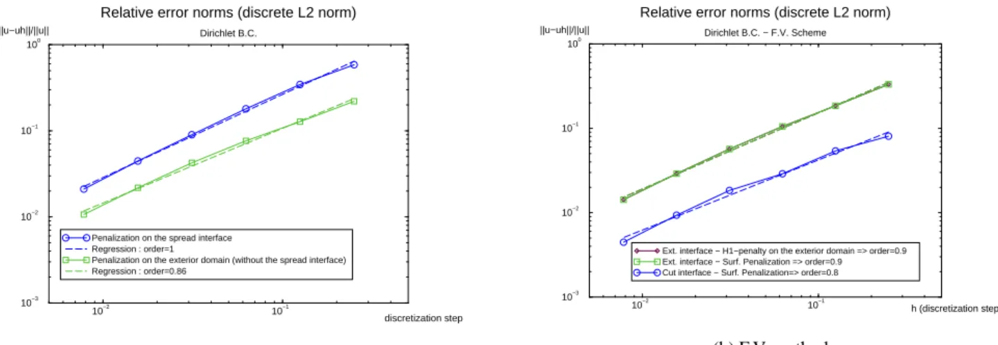
For each approach, Figure 4 represents the relative discrete L2 error norms versus the discretization step of the fictitious domain.
As excepted, the order of the method is approximatively equal to one for all the approaches since the approximation of the interface is in
✂
h✝ (for the spread as for the thin one). The interface discretization
error leads to a “global” discretization error in
✂
h✝ even if the numerical scheme error is in
✂
10−2 10−1 discretization step 10−3 10−2 10−1 100 ||u−uh||/||u||
Relative error norms (discrete L2 norm) Dirichlet B.C.
Penalization on the spread interface Regression : order=1
Penalization on the exterior domain (without the spread interface) Regression : order=0.86
(a) F.E. method
10−2 10−1 h (discretization step) 10−3 10−2 10−1 100 ||u−uh||/||u||
Relative error norms (discrete L2 norm)
Dirichlet B.C. − F.V. Scheme
Ext. interface − H1−penalty on the exterior domain => order=0.9 Ext. interface − Surf. Penalization => order=0.9 Cut interface − Surf. Penalization=> order=0.8
(b) F.V. method
Figure 4: Estimation of the discretization error for a Dirichlet B.C.
In the F.E. approach, the penalization of the exterior domain is more accurate than the penalization of the spread interface. These results strictly depend on the geometry of the physical domain. Since the discretization nodes are located on the elements vertex, nodes inside the physical domain are penalized with a spread interface penalization. In the quarter disk case, interior penalized nodes are globally farther of the physical interface than the exterior nodes.
In the F.V. approach, we can observe that, with an exterior approximated interface, the H1-penalty of the exterior domain and the surface penalization lead to the same errors. Indeed, with the H1-penalty, the solution and its gradient is penalized. So u ✞ uD on the exterior domain until the approximated
inter-face. Moreover, with a thin interface approach, the errors obtained are better for a “cut” approximated interface than for an exterior interface. The cut approximation of the interface is more precise.
The last conclusion to draw is that the effect of the H1 exterior penalization is similar with the two schemes.
As drawn on the Figure 5 the main differences between the approximated solution and the analytic one are located around the spread interface. Using the F.E. scheme, an adaptive mesh refinement is performed in this zone. At each level an exterior penalization is performed. A three-grid LDC algorithm (two refinement levels) is applied on each initial mesh. At each level, the local refinement zone is composed by all the elements of the spread interface✄ h
☎ and their neighbors. This algorithm converges
by three V-cycles.
Figure 5: Absolute error for the exterior penalization -F.E Scheme - Dirichlet case - 32x32 mesh
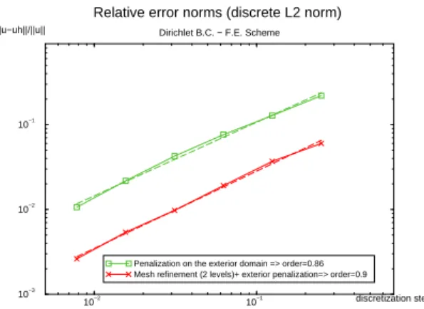
The errors computed using a three-grid mesh refinement and the ones obtained without refinement are represented on Figure 6.
10−2 10−1 discretization step 10−3 10−2 10−1 ||u−uh||/||u||
Relative error norms (discrete L2 norm)
Dirichlet B.C. − F.E. Scheme
Penalization on the exterior domain => order=0.86 Mesh refinement (2 levels)+ exterior penalization=> order=0.9
Figure 6: Relative error norms with or without refi nement - F.E. Scheme - Exterior penalization - Dirichlet case
The results obtained with a local refinement are in
✂
h✝ where h is the discretization step of the finest
refinement grid. With A.M.R., on the initial “coarse” mesh, the error obtained after correction is similar to the one obtained without A.M.R. on a mesh with a discretization step equal to the finest local grid’s one. Even if the order of the method doesn’t increase with a local refinement, the errors on the initial meshes are reduced.
3.2 Robin case
We consider the following problem:
✞ ✟✠ ✁✁ ˜u ✞ 16r 2 in ˜✠ ✂ ˜u ✂ n ✞ 0 on ˜ ☛ ✁ ✂ ˜u ✂ n ✞ u✏ 3 on ☞
Identifying with the generic formulation (1), we get: ˜a ✗ 1 ✂ ˜a✗ Id ✝✓✖ ˜f ✞ 16r 2 ✖ ✍ R ✞ 1✖ uR ✞ 0 and gR ✞ 3 ✂ Robin B✄C✄✝
The solution of this problem is :
˜u✞ 2 ✁ r
4 in ˜✠
In the F.E. approach, the characteristic parameter✏ can be estimated be several ways. In this section
we present three of them. From the equation (6), supposing that the flux carried by the spread interface and the flux carried by the physical interface are rather similar (this approximation is as much justified as the discretization step becomes small), we obtain :
✄ ☎ dS ✄ ✑ h✓✔ 1 ✏ dV (11)
The three estimations of✏ can be deduced of the equation (11):
✂
In a first approach,✏ is supposed constant on✄ h ☎ : ✏ ✞ meas ✂ ✄ h ☎ ✝ meas ✂ ☞ ✝ ✂
In the second approach, in the equation (11), the integration on✄ h
☎ is weighted by a coefficient ✁ .
This coefficient estimates the presence rate of the physical domain in each element K crossed by the boundary☞ (K ✂ ✄ h ☎ ). By construction, ✁ is constant on each K : ✁ K ✞ volume of ˜✠ included in K volume of the element K
By this way, the right hand side of (11) is integrated only on the physical domain included in✄ h ☎ . We get : ✏ K ✞ e★✁ e✄meas ✂ K✝ ✦ ✁ e✄meas ✂ ☞ ✝
The value of✏ is given by element.
This approximation of✏ is called volume weighted approximation.
✂
In the last approach, the boundary ☞ is piecewise linear approximated by a segment ☞ l K in
each element K included in ✄ h
☎ . The equation (11) is written for each of these elements K
(respect to equation (6), we use test functions v lying only on K). Using the linear approximation
☞ l✞ ✂ K✁ ✑ h✓✔ ☞ l Kof☞ , we get: ✄ ☎ l✓K dS ✄ K 1 ✏ dV Finally, ✏ K ✞ meas ✂ K✝ meas ✂ ☞ l K✝
As in the second case, the value of✏ depends on the element K.
This approach induces a local reconstruction of the interface.
For these three estimations of ✏ , the errors obtained according to the methodology described Section
2.1.2 are reported Figure 7(a).
In the F.V. approach, the characteristic parameter is estimated by two manners.
✂
Global correction : the characteristic parameter✏ is deduced from the same equation as in (11)
with a surface integral on the thin approximated interface☞ hinstead of the volume integral on the
spread interface✄ h ☎ : ✏✟✞ meas ✂ ☞ h✝ meas ✂ ☞ ✝ ✂
Local correction : A local estimation of ✏ is made in each cell K of the mesh crossed by the
immersed interface ☞ . In this case✏ K corresponds to the ratio between the sum of the measures
of the normal projections of the physical boundary ☞ on each mesh axis (x and y in 2D), and the
measure of the physical immersed interface☞ itself. In 2D, with a piecewise linear approximation ☞ lof☞ composed by a segment☞ l Kin each K crossed by☞ , we get:
✏ K ✞ cos✂ K ✏ sin✂ K
where✂ K indicates the angle between the normal direction n
☎
l✓K
of☞ l Kand the horizontal axis x.
Figure 7(b) shows the errors obtained for these two estimations of ✏ with the transfer parameters
introduced Section 2.2.2 for two kinds of thin approximation of the interface (exterior and cut approxi-mated interface).
All the F.E. variants are approximatively of order one (a little bit under). The method using a piecewise linear approximation of the interface leads to little better results but not as excepted. Some improvements are presented Section 3.3.
Concerning the F.V. variants (using a thin interface approximation), the global correction leads to an asymptotic stagnation of the error with a cut interface and then the first-order precision is lost. This stagnation disappears with the local correction (see also Figure 8(b)).
In Fig.7(b), for an exterior interface, the two estimations of ✏ seem to lead to the same errors and
then to the same first-order method. However, in Fig. 8, we can observe that for finer meshes (256 ✩ 256✖ 512 ✩ 512 cells) a stagnation appears also for a global correction since the local correction
10−2 10−1 discretization step 10−2 10−1 100 ||u−uh||/||u||
Relative error norms (discrete L2 norm) Robin B.C. − F.E. Scheme
Constant epsilon (=meas(wh,S)/meas(S)) => order=0.80 Variable epsilon (volume weighted) => order=0.84 Variable epsilon (lin. approx.) => order =0.86
(a) F.E. method
10−2 10−1 discretization step 10−2 10−1 100 ||u−uh||/||u||
Relative error norms (discrete L2 norm) Robin B.C. − F.V. Scheme − No exterior control
Global epsilon − Ext. interface => order=0.82 Local epsilon − Ext. interface => order = 0.85 Global epsilon − Cut interface => order=0.6 Local epsilon − Cut interface => order =0.9
(b) F.V. method
Figure 7: Estimation of the discretization error for a Robin B.C.
10−3 10−2 10−1 100 discretization step 10−3 10−2 10−1 100 ||u−uh||/||u||
Relative error norms (discrete L2 norm) Robin B.C. − F.V Scheme − Global epsilon
Ext. thin interface => order=0.85 Cut thin interface => order=0.6
(a) Global correction
10−3 10−2 10−1 100 discretization step 10−3 10−2 10−1 100 ||u−uh||/||u||
Relative error norms (discrete L2 norm) Robin B.C. − F.V. Scheme − Local epsilon
Ext. thin interface => order= 0.9 Cut thin interface => order= 0.9
(b) Local correction
Figure 8: Comparison between the two estimations of for a Robin B.C. with a F.V. Scheme
As in the Dirichlet case, the errors obtained with the cut interface are better as the ones obtained with an exterior interface.
For the F.E. approach, a local adaptive mesh refinement is performed on the method involving a constant epsilon (✏ ✞ mes ✁ ✑ h✓✔✄✂ mes ✁ ☎ ✂
) and a local epsilon (linear approximation ✏ K ✞
meas ✁ K✂ meas ✁ ☎ l✓K✂ ). As in the Dirichlet case, we computed a three-grid LDC algorithm, which converges by three V-cycles. The results are presented Figure 9.
Here again the refinement method has a discretization error in
✂
h✝ with h the discretization step
of the local finest grid. However, performing a constant ✏ , we observe a stagnation of the error for fine
meshes and the first-order is lost. In this case, the modelization error is reached. This modelization error seems to be due to the global estimation of ✏ (equation (11)) since no stagnation appears with a local
estimation of✏ . The modelization error for a local✏ decreases with the discretization step.
For the two interface modelling (spread and thin), a local correction is required to keep the first-order method. With a global correction, the rough estimation of✏ leads to a stagnation of the error.
10−2 10−1 discretization step 10−2
10−1
100
||u−uh||/||u||
Relative error norms (discrete L2 norm) Robin B.C. − F.E. Scheme − Constant epsilon
Constant epsilon (=meas(wh,S)/meas(S)) => order=0.8 Mesh refinement (3 grids) + constant epsilon => order=0.85
(a) Constant epsilon
10−2 10−1 discretization step 10−2 10−1 100 ||u−uh||/||u||
Relative error norms (discrete L2 norm) Robin B.C. − F.E. Scheme − Linear approximation
Lin . Approx => order=0.86
Mesh refinement (3 grids) + lin. approx => order= 0.89
(b) Local epsilon (linear approximation)
Figure 9: Relative error norms with and without refi nement - F.E. Scheme - Robin case
3.3 Some improvements
We present briefly some improvements under investigations for a Robin B.C.. Those improvements are presented for the F.E. approach.
✂
Firstly, we try to correct the equation coefficients on the spread interface. The aim of this correction is to better approximate the physical domain.
A first step is to set ✁ ef instead of f on ✄ h
☎ . In this case the source term is approximatively
integrated on the physical domain (the integration is exact for a constant f ). Figure 10(a) presents the errors obtained for the three ✏ introduced Section 3.2 with a source term weighted on the
spread interface. Figure 10(b) enables to appreciate the improvement of this approach compared to the “classic” one of Section 3.2.
10−2 10−1 discretization step 10−3 10−2 10−1 ||u−uh||/||u||
Relative error norms (discrete L2 norm) Robin B.C. − F.E. Scheme − f weighted
Constant epsilon (=meas(wh,S)/meas(S)) => order=0.88 Variable epsilon (volume weighted) => order=0.92 Variable epsilon (lin. approx.) => order =1.06
(a) Approach with a weighted source term f
10−2 10−1 discretization step 10−3 10−2 10−1 100 ||u−uh||/||u||
Relative error norms (discrete L2 norm) Robin B.C. − F.E. Scheme − f weighted or not
Constant epsilon (=meas(wh,S)/meas(S)) => order=0.80 Variable epsilon (volume weighted) => order=0.84 Variable epsilon (lin.approx.) => order =0.86 Constant epsilon−f weighted=> order = 0.88 Volume weighted epsilon − f weighted=> order = 0.92 Lin. approx. − f weighted => order =1.06
(b) Comparison of the two approaches : f weighted or not
Figure 10: Relative error norms for a weighted source term f
The correction of the source term f leads to better results for each✏ approach. Moreover, for a
con-stant✏ , the stagnation to the modelization error is reached for a 32✩ 32 mesh, without using A.M.R.
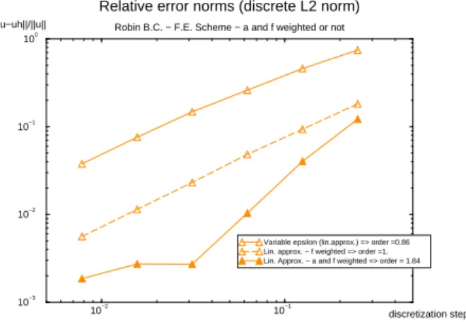
In a second step, for a local✏ (✏ linear approximated), the diffusion coefficient is also weighted
source term. Locally, on each element of the spread interface, the balance of flux of the initial problem is approximatively respected. However, we are conscious that this correction isn’t equiv-alent to a physical domain integration of the diffusion term. Results are presented on Figure 11.
10−2 10−1 discretization step 10−3 10−2 10−1 100 ||u−uh||/||u||
Relative error norms (discrete L2 norm) Robin B.C. − F.E. Scheme − a and f weighted or not
Variable epsilon (lin.approx.) => order =0.86 Lin. approx. − f weighted => order =1. Lin. Approx. − a and f weighted => order = 1.84
Figure 11: Relative error norms for a weighted diffusion coeffi cient a
This approach has a much better order as the other ones. Indeed, the order reaches almost 2. However, even with these corrections of the source term and of the diffusion coefficient, the dis-cretization error stagnates around a modelization error. With a local ✏ , this modelization error is
reduced compared to the constant✏ ’s one.
✂
Secondly, beginning from the equation (3), we computed on the spread interface the surface
inte-gral of the jump of flux :
✌ ★★ ✂ a✄✆☎ uh✝ ✄n✦✦ ☎ ☎ ☎ ✖ v ✚ ✞ ✄ ☎ ★★ ✂ a✄✆☎ uh✝ ✄n✦✦ ☎ v dS ✛ v ☎ Vh ✂ H1 ✂ ✠ ✝
On each element of the spread interface, we choose the base functions associated at each node as test functions. If we call xBthe barycenter of the immersed interface intersected in an element, the
local surface integral is approximated by an one point Gauss formula on xB. This approach needs
a local reconstruction of the interface but avoids the estimation of a characteristic parameter✏ in
order to obtain a volume integral. Following figures (Figure 12(a) and 12(b)) compare this surface integral approach (weighting the source term f and the diffusion coefficient a) with an unstructured mesh approach in term of error/discretization step and error/CPU time.
10−3 10−2 10−1 100 discretization step 10−4 10−3 10−2 10−1 ||u−uh||/||u||
Relative error norms (discrete L2 norms)
Robin B.C. − F.E. Scheme − a and f weighted
Surface integral Unstructured mesh
(a) Errors versus discretization step
0 2 4 6 8 10
time (in secondes)
10−4
10−3
10−2
10−1
||u−uh||/||u||
Relative error norms (discrete L2 norms)
Robin B.C. − F.E. Scheme − a and f weighted
Surface integral Unstructured mesh
(b) Errors versus CPU time
Figure 12: Relative error norms for a surface integral approximation
In the approximated surface integral approach, a slope break prevents from determining the order of the method. However, the errors obtained with this approach are comparable to those obtained for unstructured meshes, in term of discretization error as in term of in CPU time. Moreover, in
term of CPU time, the results presented here for the surface integral approach aren’t optimal as the software used is dedicated to unstructured meshes.
4 CONCLUSIONS
The first step of the introduction of a general fictitious domain approach to deal with structured meshes for complex industrial applications has been introduced. The fictitious domain approach introduced here don’t use local unknowns and don’t modify locally the numerical scheme. Moreover, all the usual embedded B.C. (Dirichlet, Neumann, Fourier) can be treated with these methods.
For a diffusion problem in a domain of SG’s type, we exposed :
✂
the methodology to take into account usual B.C. lying on a immersed interface using two numerical schemes : a F.E. scheme and a F.V. scheme. The two main approximated interface approaches have been tested : spread and thin interface.
✂
numerical results for Dirichlet and Robin B.C. on the immersed interface. These two cases provide satisfactory results with errors in
✂
h✝.
✂
some recent improvements in order to get better results (comparable to unstructured meshes). The results presented here give confidence for the use of fictitious domain methods in more complex industrial applications. Even if the discretization error is in
✂
h✝, the computed relative errors are rather
small.
Moreover the use of structured meshes is full of promise : meshing costs are weak, local adaptive mesh refinements are easily implemented, moving boundaries can be simulated without mesh reconstruction, fast solvers can be used...
The resolution of an advection-diffusion problem with the FDM presented here is on hand. Future works will focus on homogeneous Navier-Stokes equations for the simulation of two-phase flows in Nuclear Power Plants.
5 NOMENCLATURE
˜✄ : subscript invoking data of the physical problem
˜ ✠ : physical domain ✠ : fictitious domain ✠ e : exterior domain ☞ : immersed interface ˜ ☛ = ✁ ˜ ✠ ✁ ✠ ☛ e : exterior boundary ✄ h
☎ : spread approximated interface ☞ l : piecewise linear approximation of☞ ☞ h : thin approximated interface
✏ : characteristic parameter used to impose the immersed flux
REFERENCES
Angot, Ph. 1989. Contribution à l’étude des transferts thermiques dans des systèmes complexes;
Angot, Ph. 1999. Finite volume methods for non smooth solution of diffusion models; Application to imperfect contact problems. Numerical Methods ans Applications-Proceedings 4th Int. Conf. NMA’98,
Sofia (Bulgaria) 19-23 August 1998, pp.621-629, World Scientific Publishing.
Angot, Ph. 2003. A model of fracture for elliptic problems with flux and solution jumps. C.R. Acad. Sci.
Paris, Ser I 337 (2003) 425-430.
Angot, Ph., Caltagirone, J.-P., & Khadra, K. 1993. A comparison of locally adaptive multigrid methods: L.D.C., F.A.C.ANDF.I.C. NASA Conf. Publ. CP-3224, volume 1, pp.275-292.
Angot, Ph., Bruneau, Ch.-H., & Fabrie, P. 1999. A penalization method to take into account obstacle in incompressible viscous flows. Numerische Mathematik, 81(4):497-520.
Brezis, H. 2000. Analyse fonctionnelle, Théorie et applications. Dunod.
Cortez, R., & Minion, M. 2000. The blob projection method for immersed boundary problems. J.
Comput. Phys., 161:428-463.
Dautray, R., & Lions, J.L. 1988. Analyse mathématique et calcul numérique pour les sciences et les
techniques, vol. 1-9. Masson.
Eymard, R., Gallouët, Th., & Herbin, R. 2000. Finite Volume methods. P.G. Ciarlet, J.-L. Lions (Eds), Handbook of Numerical Analysis, vol. VII, North-Holland, pp.713-1020.
Glowinski, R., & Kuznetsov, Y. 1998. On the solution of the Dirichlet problem for linear elliptic opera-tors by a distributed Lagrange multiplier method. C.R. Acad. Sci. Paris, t.327, Seie I, pp. 693-698. Glowinski, R., Pan, T.-W., Wells, Jr.R., & Zhou, X. 1996. Wavelet and finite element solutions for the
Neumann problem using fictitious domains. Journal COmput. Phys., Vol. 126(1),pp.40-51.
Grandotto, M., & Obry, P. 1996. Calculs des écoulements diphasiques dans les échangeurs par une méthode aux éléments finis. Revue européenne des éléments finis. Volume 5, n 1/1996, pages 53 à 74. Grandotto, M., Bernard, M., Gaillard, J.P., Cheissoux, J.L., & De Langre, E. April 1989. A 3D finite element analysis for solving two phase flow problems in PWR steam generators. In: 7th International
Conference on Finite Element Methods in Flow Problems, Huntsville, Alabama, USA.
Hackbusch, W. 1984. Local Defect Correction Method and Domain Decomposition Techniques. volume
5 of Computing Suppl.,pages 89-113, Springer-Verlag (Wien).
Hackbusch, W. 1985. Multi-grid Methods and applications. Series in computer mathematics,
Springer-Verlag.
Khadra, K., Angot, Ph., Parneix, S., & Caltagirone, J.-P. 2000. Fictitious domain approach for numerical modelling of Navier-Stokes equations. Int. J. Numer. Meth. in Fluids, Vol. 34(8): 651-684.
Kopˇcenov, V.D. 1974. (in Russian). A method of fictitious domains for the second and third value problems. Trudy Mat. Inst. Steklov, Vol 131, pp.119-127.
Latché, J.-C. submitted (october 2003). A fictitious degrees of freedom finite element method for free surface flows. Mathematical Modelling and Numerical Analysis.
Leveque, R.J., & Li, Z. 1994. The immersed interface method for elliptic equations with discontinuous coefficients and singular sources. SIAM J. Numer. Anal., 31:1019-1044.
Marchuk, G.I. 1982 (1rst ed. 1975). Methods of Numerical Mathematics. Application of Math. 2, Springer-Verlag New York.
McCorquodale, P., Colella, P., & Johansen, H. 2001. A cartesian grid embedded boundary method for the heat equation on irregular domains. J. Comput. Phys., 173:620-635.
Ramière, I., Angot, Ph., & Belliard, M. in preparation. Using a fictitious domain approach for solving a diffusion problem. in preparation.
Saul’ev, V.K. 1963. (in Russian). On the solution of some boundary value problems on high performance computers by fictitious domain method. Siberian Math. Jounral, 4(4):912-925.
Ye, T., Mittal, R., Udaykumar, H.S., & Shyy, W. 1999. An accurate cartesian grid method for viscous incompressible flows with complex immersed boundaries. J. Comput. Phys., 156:209-240.