HAL Id: halshs-00115791
https://halshs.archives-ouvertes.fr/halshs-00115791
Submitted on 23 Nov 2006
HAL is a multi-disciplinary open access
archive for the deposit and dissemination of sci-entific research documents, whether they are pub-lished or not. The documents may come from teaching and research institutions in France or
L’archive ouverte pluridisciplinaire HAL, est destinée au dépôt et à la diffusion de documents scientifiques de niveau recherche, publiés ou non, émanant des établissements d’enseignement et de recherche français ou étrangers, des laboratoires
Stage-specific technology shocks and employment:
Could we reconcile with the RBC models?
Chahnez Boudaya
To cite this version:
Chahnez Boudaya. Stage-specific technology shocks and employment: Could we reconcile with the RBC models?. 2006. �halshs-00115791�
Maison des Sciences Économiques, 106-112 boulevard de L'Hôpital, 75647 Paris Cedex 13
Centre d’Economie de la Sorbonne
UMR 8174
Stage-Specific Technology Shocks and Employment!: Could we Reconcile
with the RBC Models!?
Chahnez BOUDAYA
Stage-Speci…c Technology Shocks and
Employment: Could We Reconcile with the
RBC Models?
Chahnez Boudaya
y
I would like to thank Nooman Rebei for technical support and stimulating suggestions. The usual disclaimer applies.
yCentre d’Economie de la Sorbonne (EUREQua), Université Paris1-Sorbonne, Maison
des Sciences Economiques 106-112 Bd de l’Hôpital 75013 Paris. E-mail: [email protected].
Résumé
L’auteur examine la dynamique d’un modèle à deux stades de production rattachés par une structure verticale input-output, et où chaque stade est sujet à un choc technologique qui lui est propre. Par ailleurs, le modèle présente des rigidités nominales de prix et de salaires ainsi que des coûts d’ajustement d’emploi et de capital. Les résultats de l’estimation sur des données d’après-guerre révèlent que les prédictions du modèle au chapitre de l’ajustement de l’emploi aux chocs technologiques sont variées: i) Les heures travaillées baissent de façon persistante suivant un choc technologique positif au stade …nal et ii) augmentent suite à un choc technologique positif au stade intermédiaire.
Classi…cation JEL:E24, E32, E52
Mots-clés: Modèles RBC, Rigidités de prix et de salaires, Stades de pro-duction, Chocs technologiques.
Abstract
This paper analyses the response of labor input to technology shocks in an estimated two-stage production framework with both price and wage stickiness and stage-speci…c shocks to productivity. The model features a vertical input-output structure with imperfect mobility of labor across stages. The estimation uses the maximum likelihood technique applied to the post-war US data. the main …ndings could easily match the standard RBC models predictions: A shock to productivity in the intermediate good production stage i) leads to an increase in both stage-speci…c labor and the aggregate labor and ii) explains a large proportion of the volatility of both the real GDP and the aggregate labor. Besides, regarding the output-labor correlation, the model does a very good job in matching the data.
JEL classi…cation: E24, E32, E52
Keywords: RBC models, Sticky prices, Sticky wages, Production chain, Employment, Technology shocks, Sectoral comovements.
1
Introduction
It is an old idea presented at least from Means (1935) that,
"...in an industrialized economy the relationship between money, prices and output is tied to the interdependence of …rms at each stage of production. This led many to conclude that there is a conjunction between aggregate ‡uctuations and an input-output structure..." (Huang and Liu 2001)
In lines with Means’ claim, a large strand of literature emerging from multi-sector models has attracted a growing interest about the transmission of business cycle shocks through a horizontal (vertical) roundabout input-output structure within a single (multiple) stage(s) of production. For in-stance, Long and Plosser (1983,1987) speci…ed a six-sector model of the econ-omy with intermediate input linkages and uncorrelated sector-speci…c shocks to examine the transmission mechanisms of real shocks. Besides, Bergin and Feenstra (2000) show that the interactions between staggered-price setting and the real rigidity introduced through a non-CES aggregation technology and a roundabout input-output structure help generate real persistence fol-lowing monetary shocks. Also, Basu (1995) focused on the transmission of monetary shocks in a roundabout input-output production structure. In the same vein, Huang, Liu and Phaneuf (2004) examine the cyclical behavior of real wages in response to monetary shocks in a DSGE model with either nominal wage and/or price rigidities and a horizontal input-output structure with a single stage of production. By contrast, Boudaya (2005) focuses on technology shocks e¤ects on hours worked in a New Keynesian framework with staggered price settings à la Calvo. It sorts out from the interest about the horizontal input-output structure that i) it improves the models’ability to generate variables responses persistence; and ii) it reinforces the rigidities e¤ects in the model. Recent papers on this topic were interested instead, in the shocks transmission in models with vertical input-output structure. For instance, Blanchard (1983) was interested to explain the sluggish adjustment of prices. Huang and Liu (2001) propose a model that features a vertical input-output structure with staggered price contracts at each stage of pro-duction to generate the observed persistence of aggregate output in response to monetary shocks. Also, Huang and Liu (2004) exmines the optimal mon-etary policy in a DSGE framework with two stages of production. Recently,
another strand of literature follows the lead of Gali (1999) and was con-cerned to investigate the controversial e¤ects of a technology improvement on output, labor and other economic variables. The seminal paper of Gali (1999) identi…es technology shocks as the only shocks that have an e¤ect on labor productivity in the long run and estimates a persistent decline of hours in response to a positive technology shock. As Gali points out, this result is more consistent with the predictions of a dynamic stochastic gen-eral equilibrium model (DSGE) with sticky prices than those of standard Business Cycle models, as long as monetary policy is not too accommodative for technology shocks. There have been other attempts that have reached similar conclusions (see for example Kiley (1998), Basu, Fernald and Kim-ball (1998), Francis and Ramey (2001) and others). For instance, Francis and Ramey (2003) concluded that "...technology-driven real business cycle hypothesis is dead...". In a recent paper, Christiano, Eichenbaum and Vig-fusson (2003) challenge these empirical results. Using the same identifying assumption as Gali (1999), they …nd evidence that a technology shock drives hours worked up, not down. In the same way, Langot (1997) examines the e¤ects of both aggregate and sectoral productivity shocks in a job-serach model with two sectors. While an aggregate shock increases employment in both sectors, a sectoral shock have opposite e¤ects depending on sector hit by the shock.
Both strands of literature have motivated this empirical work. The pur-pose of the present paper is twofold. First, it tries to investigate whether stage-speci…c technology shocks in a dynamic general equilibrium model with both price and wage rigidities and two stages linked by a vertical input-output production structure, could reconcile with the standard RBC theory in terms of aggregate variables patterns. The prediction of a positive short run comovement between productivity, output and employment in response to technology shocks lies at the root of the ability of an RBC model to repli-cate some central features of observed aggregate ‡uctuations, while relying on exogenous variations in technology as the only (or, at least the dominant) driving force. Second, I focus on whether technology shocks could be consid-ered as the main source of ‡uctuations in aggregate output and other main variables.
I build on Boudaya (2005) and Huang and Liu (2001, 2004). The …rst one uses an horizontal input-output production structure within one stage of production to show that i) for plausible values of the intermediate input share, a favorable technology shock leads to a short-run decline in labor
in-put regardless of monetary policy considered and that ii) the initial decline becomes more important as the intermediate input share grows because of a strong substitution e¤ect between the intermediate goods and the labor input. In fact, taking into account the presence of intermediate goods in-troduces on one hand, more price rigidities in the model and thus makes variables adjust more slowly to the shocks; and on the other hand yields to a substitution mechanism between intermediate goods and labor which causes the later to fall in response to a favorable technology shock, when combined with more price rigidities. Huang and Liu (2001) consider the production of a …nal good through multiple stages of processing and introduce staggered price contracts at each stage to show that output response to a monetary shock is more persistent, the greater the number of stages of production and the larger the share of intermediate inputs. On the other hand, Huang and Liu (2004) introduce two stages in the production scheme to examine the op-timal monetary policy in a model without capital accumulation. The present paper, however di¤ers from Boudaya (2005) and Huang and Liu (2001, 2004) in several points. First, it takes into account the two-stages productive frame-work but with capital accumulation. Second, as in Boudaya (2005), I focus on a Taylor rule. Besides, I introduce nominal wage rigidities in addition to staggered price settings.
In order to achieve my goal, I construct a two-stage productive dynamic stochastic general equilibrium model that features monopolistic competition in both the …nal goods market and the labor market, with …rms setting nominal prices for their products and households setting nominal wages for their labor skills.
The main …ndings can be brie‡y summarized as follows. First, a 1% shock to technology in the intermediate-good sector leads to a persistent increase in labor input in both sectors. Second, it explains the major part of the volatil-ity of …nal output, intermediate good, investment, real wages, in‡ation and labor input in the intermediate-good sector. Consequently, if I consider a pro-ductivity shock in the intermediate-good sector as the only source of business ‡uctuations, my model of price rigidities could reconcile with the predictions of standard business cycle models!! So, technology shocks do matter as the driving force of aggregate ‡uctuations. Furthermore, a productivity shock in both …nal goods and intermediate goods stage could explain about 65% of output variations and 90% of aggregate employment ‡uctuations despite all rigidities in my model. This result contrasts sharply with Gali (1999) con-clusions that only non-technological shocks could explain output variability
in a price rigidities framework.
The paper is organized into …ve sections. Section II presents the model within two productive stages, a productivity shock speci…c to each stage, a money-demand shock. Besides, I introduce labor adjustment costs, staggered prices and wages setting à la Calvo. The monetary policy is governed by a Taylor rule. Section III reports the estimation procedure and the results. In section IV, I provide the impulse responses and report the performance of the model via moment comparisons. Section V concludes.
2
The model
The economy is composed by a large number of in…nitely lived households with di¤erent labor skills, which are imperfect substitutes for each other in the production process, and two stage-production linked by a vertical input-output structure. Thus, …nal consumption goods are produced through two stages of processing, from intermediate goods to …nished goods. At each stage, there is a continuum of monopolistically competitive …rms producing di¤erentiated goods. There is one shock to technology at each stage. Fol-lowing Huang and Liu (2004), I assume that monetary authorities cannot distinguish the source of technological innovation when it happens.
2.1
Households
Households o¤er di¤erentiated labor skills. I consider a continuum of di¤erent households indexed by i. Besides, household i has preferences de…ned over real consumption, Ct(i), real money balances,
Mt(i)
Pt and leisure, 1 Nt(i; :).
The expected utility function of a representative consumer-worker i is spec-i…ed as: U0 = E0 1 X t=0 t " 1log Ct(i) 1 + b 1 t Mt(i) Pt 1! + log(1 Nt(i; :)) #
where and are positive structural parameters denoting the constant elasticity of substitution between consumption and real balances, and the weight on leisure in the utility function, respectively and 2 (0; 1) is the discount factor. Total time available to the household in the period is nor-malized to one.
Shock bt is interpreted as a shock to money demand , and it follows the
…rst-order autoregressive process:
log bt= (1 b) log b + blog bt 1+ "bt;
where b 2 ( 1; 1), and the serially uncorrelated shock "bt is normally
distributed with zero mean and standard deviation b.
The representative household i carries real balances and bonds Bt(i)into
period t. At the beginning of the period, she receives lump-sum nominal transfer Tt(i)from monetary authority in addition to work revenues, capital
returns and nominal pro…ts Dt(i)as a dividend from each intermediate
goods-producing …rm j. Next, the household’s bonds mature, providing it with Bt(i) additional units of money. The household uses some of this money to
purchase Bt+1(i) new bonds at the nominal cost BRt(i)
t 1; hence, Rt 1 denotes
the gross nominal interest rate between t-1 and t. Besides, household i uses some of her funds to purchase …nal good consumption at price Pt. Moreover,
I assume that it is costly to intertemporally adjust the capital stock, since there are adjustment costs speci…ed as:
CACt(i) = 2 Kt+1(i) Kt(i) 1 2 Kt(i)
where > 0 is the capital-adjustment cost parameter. The budget constraint of household i is given by:
Ct(i) +
Mt(i)
Pt
+Bt+1(i) Pt
+ Kt+1(i) (1 )Kt(i) + CACt(i)
= Wt(i) Pt Nt(i) + Rk;t Pt Kt(i) + Mt 1(i) Pt + Rt 1 Bt(i) Pt + Tt Pt + Dt Pt
where 2 (0; 1) denotes the constant capital depreciation rate.
Each household chooses Ct(i), Mt(i), Bt+1(i), Kt+1(i) and Wt(i) (if the
household is allowed to change its wage) to maximize the expected discounted sum of her utility ‡ows subject to the budget constraint and to …rms’demand for her labor type i.
The e¤ective labor input in the production process of a typical …rm is given by a CES function of the quantities of the di¤erent types of labor hired:
Nt = Z 1 0 Nt(i; :) 1 di 1 ;
where 1denotes the elasticity of substitution between di¤erentiated labor skills. The total demand of all …rms for labor skill i is given by:
Nt(i; :) =
Wt(i)
Wt
Nt; (1)
Ntis the aggregate employment and Wtis the aggregate wage index given
by: Wt= Z 1 0 Wt(i)1 di 1 1
Households are price takers in the goods market and monopolistic com-petitors in the labor market. They set wages for their labor skills, taking the labor demand schedule 1 as given.
The …rst-order conditions for this problem are: Ct(i) 1 Ct(i) 1 + b 1 t Mt(i) Pt 1 = t (2) b 1 t Mt(i) Pt 1 Ct(i) 1 + b 1 t Mt(i) Pt 1 = t 1 1 Rt (3) Et t+1 t " rkt+1+ 1 + Kt+2(i) Kt+1(i) 1 Kt+2(i) Kt+1(i) 2 Kt+2(i) Kt+1(i) 1 2# = 1+ Kt+1(i) Kt(i) 1 (4) t= RtEt t+1 y;t+1 (5) where t is the Lagrangian multiplier associated with the budget
Following Ireland (1997) and Kim (2000), equations (1) and (2) can be combined with equation (5) to approximate a real money-demand function of the form: log Mt Pt = log(Ct) + 1 1 log(bt) 1 1log(rt) (6) where rt is the net nominal interest rate between t and t+1 (rt= Rt 1), 1
1 is the interest elasticity of money-demand.
In addition, there is a …rst-order condition for setting the nominal wage when the household is allowed to do so. This happens with probability dw
at the beginning of each period.
f Wt(i) = ( 1) EtP1m=0( dw)m1 NNt+m(i) t+m(i) EtP1m=0( dw)mNt+m(i) t+m(i)P1 t+m (7) Therefore, the household’s optimal wage is a constant markup over the ratio of weighted marginal utilities of leisure to marginal utilities of income within the duration of wage contracts.
The wage index evolves over time according to the recursive equation given by:
Wt = [dwWt 11 + (1 dW) fWt 1
]11 (8)
where fWt is the average wage of those workers who revise their wage at
time t.
This condition together with (7) allows to derive the following Phillips curve: ^w;t= Et^w;t+1+ (1 dw)(1 dw ) dw N 1 NN^t ^ t w^t (9)
The term in square brackets measures the marginal rate of substitution (the real marginal cost to workers of their work e¤ort) minus the real wage.
The wage in‡ation is de…ned by
w;t
Wt
Wt 1
2.2
Firms
I consider two types of monopolistically competitive …rms: intermediate goods-producing …rms and materials-producing …rms. Final goods sector and intermediate goods sector are linked by a vertical input-output struc-ture. The prices of both intermediate production inputs and …nal consump-tion goods are determined by staggered nominal contracts à la Calvo with probabilities dz and dy of survival in each period. Therefore, both the price
index of intermediate goods (which corresponds broadly to the PPI) and that of …nished goods (which corresponds to the CPI ) are sticky in the model.
The …nal good, Yt, is a composite of di¤erentiated …nished goods. In
particular, Yt= Z 1 0 Yt(j) y 1 y dj y y 1
where y 2 (1; 1) denotes the elasticity of substitution between the
dif-ferentiated …nished goods, Yt(j) is the output of …nished good j.
To produce a type j (j 2 [0; 1]) …nished good requires inputs of labor, Ny;t(i; j), capital, Ky;t(j), and a composite of intermediate goods (materials),
Zt(j)with a constant returns to scale technology given by:
Yt(j) = Zt(j) Ay;tK
y
y;tNy;t(i; j)1 y 1 (11) where Zt = R1 0 Zt(l) z 1 z dl z z 1
denotes the input of composite inter-mediate goods used by j, z > 1 is the elasticity of substitution between
di¤erentiated intermediate goods, and Ay;t is a productivity shock to the
…nished good sector.
The parameters y and are positive and less than one.
Intermediate …rm l rents capital, Kz;t(l), hires workers, Nz;t(l) and
com-bines the two factors to produce a quantity Zt(l) of intermediate good
fol-lowing the constant-return-to-scale technology:
Zt(l) = Az;tKz;tzNz;t(i; l)1 z (12)
Ay;t is a productivity shock to the intermediate good sector, z 2 (0; 1)
is the share of capital.
log(Ak;t) = (1 A;k) log(Ak) + A;klog(Ak;t 1) + "k;t; k2 fy; lg; (13)
where "y;t and "z;t are mean-zero, i.i.d. normal processes that are
mutu-ally independent, with …nite variances given by 2
y and 2z, respectively.
Firms are price-takers in the input markets and monopolistic competitors in the product markets. At each processing stage, prices are set optimally in a randomly staggered fashion as suggested by Calvo (1983). More speci…cally, …rms in the …nished good sector and the intermediate good sector can reset their prices in any given period only with the probability (1 y)and (1 z),
respectively, independently of other …rms and of the time elapsed since the last adjustment. Thus, a measure (1 k), k 2 fy; zg of producers reset their
prices each period , while a fraction k keeps their prices unchanged.
The maximization problem for the intermediate goods-producing …rm j is : max fKy;t(j);Ny;t(:;j)g Et 1 X q=0 ( dy)q t+q t Dy;t+q(j) Pt+q subject to:
Dy;t(j) = Pt(j)Yt(j) Rk;tKy;t(j)
Z 1 0
Wt(i)Ny;t(i; j)di LACy;t(j) Pz;tZt(j)
Yt(j) = Pt(j) Pt y Yt and (11)
where t is the marginal utility of wealth for a household i and LACt(j)
is the labor adjustment cost in terms of proportional loss of output. I assume a convex form with respect to labor increase.
LACy;t(j) = 'y 2 Ny;t(j) Ny;t 1(j) 1 2 Yt(j); 'y > 0
Labor adjustment costs are introduced to prevent from perfect mobility of labor between the two sectors.
wt = (1 y)(1 ) y;t(j) Yt(j) Ny;t(j) 'yYt(j) Ny;t 1(j)2 (Ny;t(j) Ny;t 1(j)) + 'yEt[ t+1 t (Ny;t+1(j) Ny;t(j)) Yt+1(j) Ny;t(j)2 ] (14) rk;t = y(1 ) 1 y;t(j) Yt(j) Ky;t(j) (15) pz;t= 1 y;t(j) Yt(j) Zt(j) (16) where Wt
Pt = wt is the real wage, yt is the real markup, rk;t is the real
capital return, and pz;t is the real price for the intermediate input, Zt.
I assume that prices ~Py;t(j) are determined by a Calvo contract with a
probability dy that the …rm j keeps its price unchanged at period t. In that
case, the aggregate price level is given by:
Py;t= h dyP 1 y y;t 1 + (1 dy) ~P 1 y y;t i 1 1 y (17) where Py;t is the logarithm of aggregate price level in the …nal good sector
and Py;t is the logarithm of the price …xed by the …rms adjusting their prices
in t. The optimization problem of the …rm adjusting its price is the following:
max Py;t 1 X q=0 ( dy)qEt " t+q t Py;t(j) 1 y;t+q(j) Py;t+q Yt+q(j) #
subject to (11) and the following demand function:
Yt+q(j) =
Py;t(j)
Py;t+q "
Yt+q
Py;t(j) determines ~Py;t at the optimum. The …rst order condition with
respect to Py;t(j)is:
~ Py;t(j) = y y 1 EtP1q=0( dy)q t+qt Yt+q(j) 1 yt+q(j) Et P1 q=0( dy)q t+qt Yt+q(j)Py;t+q1 (18)
The previous equation relates the optimal price to the expected future price of the …nal good and to the expected future real marginal costs.
This condition, together with (17) allow to derive the following log-linearized New Phillips Curve at the symmetric equilibrium:
^y;t= Et^y;t+1 (1 dy)(1 dy ) dy ^y;t; (19) where y;t = Py;t
Py;t 1 is the in‡ation rate in the …nal-good sector, and ^y;t
corresponds to the percentage deviation of the in‡ation rate in the …nal-good sector from its steady state level.
Similarly, the intermediate goods-producing …rm l maximizes:
M axEt 1 X q=0 ( dz)q( t+q t )Dz;t+q(l) Pz;t+q subject to: Dz;t(l) = Pz;t(l)Zt(l) Rk;tKz;t(l) Z 1 0
Wt(i)Nz;t(i; l)di LACz;t(l);
and the equation (12)
Labor adjustment costs, LAC(l), are de…ned by
LACz;t(l) = 'z 2 Nz;t(l) Nz;t 1(l) 1 2 Zt(l); 'z > 0:
The …rst order conditions for this maximization problem are:
wt = (1 z) 1 z;t(l) Zt(l) Nz;t(l) 'z Zt(l) Nz;t 1(l)2 (Nz;t(l) Nz;t 1(l)) + 'zEt[ t+1 t (Nz;t+1(l) Nz;t(l)) Zt+1(l) Nz;t(l)2 ] (20) rk;t = z 1 z;t(l) Zt(l) Kz;t(l) (21) I assume that prices ~Pz;t(l) are determined by a Calvo contract with a
probability dz that the …rm l keeps its price unchanged at period t. In that
Pz;t = h dzPz;t 11 z + (1 dz) ~Pz;t1 z i 1 1 z (22) where Pz;t is the logarithm of aggregate price level and ~Pz;t is the logarithm
of the price …xed by the …rms adjusting their prices in t. The optimization problem of the …rm adjusting its price is the following:
~ Pz;t(l) = z z 1 Et P1 q=0( dz)q t+qt Zt+q(l) 1 zt+q(l) Et P1 q=0( dz)q t+qt Zt+q(l)P 1 z;t+l (23) This condition, together with (22) allow to derive the following log-linearized New Phillips Curve:
^z;t= Et^z;t+1 (1 dz)(1 dz ) dz ^z;t (24) where z;t = Pz;t Pz;t 1 (25)
2.3
The monetary authority
The central bank manages the short-term nominal interest rate, Rt, in
re-sponse to ‡uctuations in …nal-good in‡ation, y;t, and output, yt. The
inter-est rate reaction function of the central bank is given by: log Rt R = % log y;t y + %ylog yt y + vt; (26) and vt = %vvt 1+ "Rt; (27)
where y and y are the steady-state values of y;t and yt, R is the
steady-state value of the gross nominal interest rate, and vt is a zero-mean, serially
correlated monetary policy shock with standard deviation v. The error
term, "Rt, arises from the fact that the central bank can control short-term
interest rates only indirectly by setting the bank rate. The error term thus re‡ects developments in money and …nancial markets that are not explicitly captured by my model which is assumed to be i.i.d. with a standard deviation
2.4
Closing the model
When I consider the symmetric equilibrium, the market cleaning condition requires:
Kt= Ky;t+ Kz;t (28)
Nt= Ny;t+ Nz;t (29)
Yt= Ct+ It (30)
2.5
Equilibrium
For h = y; z, an equilibrium consists of the following set of allocations: Ct; Nt; Bt; mt; Kt+1; Yt; It; Zt; Kh;t; Nh;t; h;t; w;t; pz;t; wt; rk;t; h;t; Rt , that
sat-isfy the following conditions: (i) the household’s allocations solve its utility maximization problem; (ii) each …nished good producer’s allocations and price solve its pro…t maximization problem taking the wage and all prices but its own as given; (iii) each intermediate good producer’s allocations and price solve its pro…t maximization problem; and (iv) all markets clear.
Steady state details are reported in appendix A. The full-system of log-linearized equations is reported in appendix B.
3
Estimation
3.1
Estimation methodology and data
To solve the model, I log-linearize the equilibrium conditions around a sym-metric steady state where all variables are constant. In particular, I as-sume that the steady-state domestic gross in‡ation is equal to 1. Standard techniques are then used to solve the linearized system, which leads to the following state space representation:
St = ASt 1+ B t; (31)
Yt = CSt; (32)
where the vector St keeps track of the model’s predetermined and exogenous
the Kalman …lter to evaluate the likelihood function associated with the state space solution. The structural parameters are estimated by maximizing the likelihood function.1 The series used in the estimation are the nominal
inter-est rate, the in‡ation rate, the real consumption, the real money balances, and the real wages.2
The model is estimated using U.S. quarterly data running from 1964Q1 through 2004Q4. The nominal interest rate is measured by the 3-month Treasury Bill Rate. In‡ation is calculated as the changes in the consumer price index, considered as a the …nal-good price. Consumption is measured by real personal consumption expenditures. Real money balances are cal-culated by dividing the M2 money stock by the consumer price index. The real wage is measured by the ratio of the average hourly earnings over the consumer price index. All these data, except for the interest rate, are sea-sonally adjusted. Consumption and real money balances are divided by the number of the civilian population. All series except for the interest rate and the in‡ation rate, are logged and detrended using the HP …lter.
3.2
Parameter estimates
As is typically the case with the maximum-likelihood estimation of relatively large structural models, it is di¢ cult to obtain sensible estimates of all struc-tural parameters, either because some of them are poorly identi…able or be-cause the complexity of the objective function is such that the optimization algorithm fails to locate the maximum and eventually crashes. To deal with this issue, some parameters have to be calibrated prior to the estimation. Particularly, the subjective discount rate, , is set to 0:995, which implies an annual real interest rate of 2 per cent in the steady state. The intertemporal elasticity of substitution for labor is set to 1, then the weight on leisure in the utility function, , is calibrated so that the representative household spends about one third of its total time working in the steady state. The constant
1The maximum likelihood technique uses the methods outlined by Hamilton (1994, Ch.
13).
2Note that the number of variables included in the estimation procedure is …ve, however
we only consider four shocks in the model. With more than four observable variables, the system becomes stochastically singular and the maximum likelihood procedure fails. See Ingram, Kocherlakota and Savin (1994).To make the estimation exercise feasible we need the same number of observed variables as the number of shocks. Therefore, we include an additional measurment error, corresponding to the CPI in‡ation rate variable, as in Ireland (2003).
elasticity of substitution between real consumption and real balances, , is calibrated to 0:1 which is consistent with the estimates of Ireland (1997) and Kim (2000). The depreciation rate of physical capital is chosen to be 0:025. Setting = # = 8 gives a steady-state markup of 14 per cent. This corresponds well to the estimates in the empirical literature between 10 per cent and 20 per cent (see, for example, Basu 1995). The parameter gives the elasticity of substitution across di¤erent labour types in the production of individual domestic intermediate goods. The value = 6 corresponds to estimates from microdata in Gri¢ n (1992).3
Estimation results are reported in Table 1. Looking …rst at the auto-correlation coe¢ cients for the exogenous variables, the one governing the persistence for the …nal-good technology shock is smaller than the one for the intermediate-good shock. The data seem to prefer a version of the model where the supply shock on the production of materials is closer to a unit root. This can lead to some extent to a way of identifying sectoral supply shocks in a purely empirical framework. The estimate of %v = 0:5545 tells
that the unpredictable intervention of the monetary authority is mildly per-sistent. Moreover, the money demand is very persistent which is consistent with the results by Kim (1999). Note that, all the standard deviations of shocks are moderate and statistically signi…cant. In addition, the shock on Ay;t is almost three times as volatile as the shock on Az;t.
The large and signi…cant estimate of dw = 0:8295, corresponding to a
wage contract of slightly less than 6 quarters in average, suggests that the main nominal rigidity in the model is coming from the wage side. This re-sult echoes the one reported by Christiano, Eichenbaum, and Evans (2003), a study that relies on an other technique of estimation.4 Finally, and in-terestingly, the estimates of dy = 0:4341 and dz = 0:3677 all appear small
compared to the literature. The latter result shows that, on the one hand, a model combining both wage and price stickiness leads to lower price contract length. On the other hand, when I include vertical input-output structure of the production process I need less stickiness in the goods pricing side to …t
3It also agrees with the value estimated in Ambler, Guay, and Phaneuf (2003) using
ag-gregate time-series data. They succeed in estimating the value of the equivalent parameter in their model by calibrating the equivalent of the dwparameter.
4Christiano, Eichenbaum, and Evans (2003) use a di¤erent technique based on matching
conditional moments corresponding to impulse-response function to a monetary shock identi…ed in a structural VAR, and they estimate simultaneously the degrees of wage and price stickiness.
the data.
The capital adjustment cost parameter estimate is statistically signi…cant and equal to 4:2646, which is reasonable in terms of matching the volatility of investment in my model. The estimates of 'y = 0:5533 and 'z = 6:4969
imply that the …nal-good …rms can adjust more easily labor factor than the intermediate-sector ones. Unfortunately, as far as I know data on sectoral labor is not available to corroborate this result, but given that my model is estimated I can interpret the result as a fact even if there is no similar conclusions in some micro studies. Finally, the shares of capital estimates in both …nal good sector and intermediate good sector, y and z are equal to
0:3025 and 0:2567 respectively. These values appear to be consistent with the calibrated values assigned to these parameters in Kydland and Prescott (1982), Cooley and Hansen (1989), and other business cycles studies.
4
Dynamic e¤ects of the structural shocks
4.1
Variance decomposition
The best starting point is the set of variance decompositions, the contribu-tion of each source of innovacontribu-tions to the variance of each endogenous variable. Two main results emerge from table 1: i) innovations to technology in the intermediate-good sector account for most of the variance of …nal output (54%), intermediate good (80%), investment (66%), aggregate (50%) and intermediate-good sector (57%) employment, real wages (78%), nominal in-terest rates (98%) and in‡ation (88% for y;t, 96% for z;tand 99% for w;t);
while ii) innovations to …nal-good sector technology explains the most of the variance of consumption (42%).
4.2
Impulse-response functions
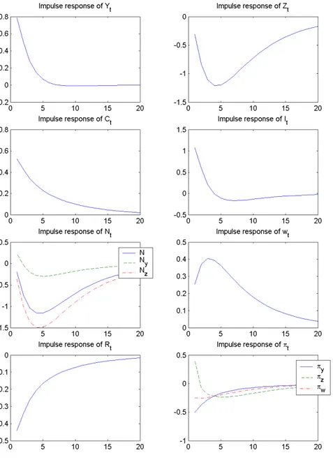
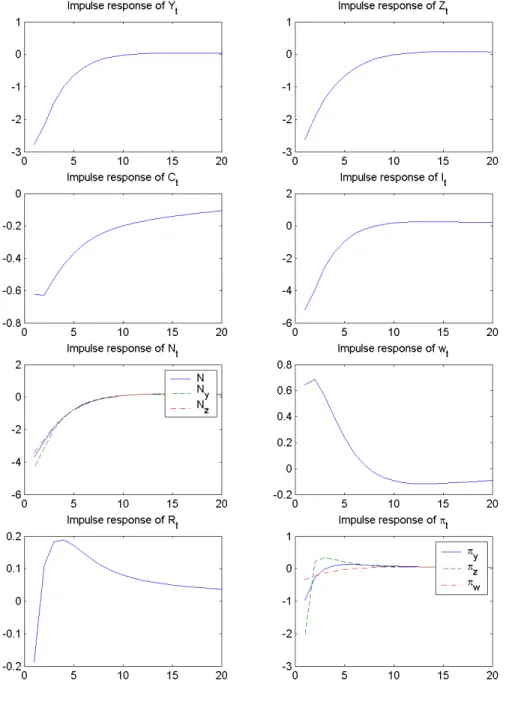
Given the results for variance decompositions, I focus mainly on the re-sponses to innovations to technology in both the …nal-good sector and the intermediate-good one. I will discuss brie‡y responses to other innovations. Figure 1 plots the impulse response functions of …nal output, intermediate input, consumption, investment, aggregate and sector-speci…c labor input, real wages, nominal interest rates and in‡ation to a 1% shock to technology in the …nal good sector. The …nal output and the real wages show a
persis-tent increase (the response of real wages is hump-shaped). In the presence of intermediate input production structure, a positive supply shock leads to a persistent decline in the inputs demand level in the …nal-good sector (see Boudaya (2005)). In fact, all inputs become more productive such that the …nal good-producing …rms could reach the same level of …nal output with less input. With labor adjustment cost, the …rms adjust their labor demand gradually (the impulse-response is hump-shaped). Consequently, the increase in real wages following a positive technology shock is less important (0.25% initially), then the wealth e¤ect dominates the substitution e¤ect. Thus, labor supply is reduced in the short run. Besides, less demand for intermedi-ate good needs less labor in the mintermedi-aterials sector. As a result, the aggregintermedi-ate employment level drops sharply. Moreover, as a favorable technology shock reduces both the …rms price level and their real marginal cost, the …nal-good sector and the real wages in‡ation decrease. The monetary authorities react by lowering the nominal interest rate.
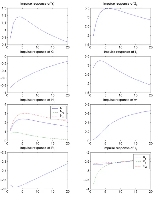
Figure 2 plots the responses of the considered variables to a 1% shock to productivity in the intermediate-good sector. The intermediate good shows a persistent increase. This needs more labor input. I should note that the estimate of the degree of price stickiness in the intermediate-good sector is too weak (0.36) which corresponds to a one quarter contract duration. Figure 7 displays the labor input sensitivity to variations in the degree of price stickiness. It sorts out from the bottom right panel that labor input Lz;t
could decline in response to a positive technology shock in the intermediate-good sector only for high and implausible values of dz. Besides, a favorable
productivity shock in the materials sector, Az;t represents a positive supply
shock in the market for intermediate goods and should result in a reduction of the relative price of intermediate goods. As a result, real wages increase. Moreover, labor would move to the sector in which productivity is higher (in that case to the intermediate-good sector) which reinforces the increase in labor input Nz;t. As the sector-speci…c employment levels are given to
move together (as shown by the unconditional correlations with aggregate employment)5, the …nal-good sector employment increases but by less than the increase in that of intermediate-good sector.
Figure 3 shows the dynamic e¤ects of a monetary policy shock on the key variables. An expansionary monetary policy shock of 1% tends to decrease
5This fact is also emphasized by Hornstein and Prachnik (1997), in a two-sector model
the investment level, the output, the intermediate goods, the consumption and the labor input. The real wages are countercyclical.
In …gure 4, I plot the impulse-responses to a 1% money demand shock. All variables, excepting real wages and nominal interest rates show a persistent decrease.
4.3
Unconditional moments
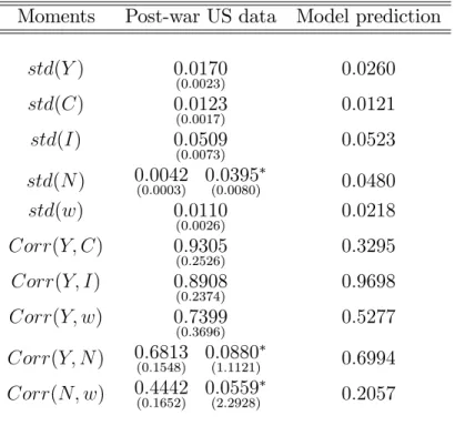
In the postwar U.S. observed data, output, consumption, investment, real wages and employment move together, with investment being much more volatile than output (3 times as volatile). Table 3 reports some second or-der unconditional moments predicted by the model. While it does a good job to replicate the observed comovement and the volatility of consumption and investment for the postwar U.S data, the model economy exaggerates the qualitative pattern of relative volatilities of output, employment and real wages. However, I also show that the model economy is broadly consistent with the observed unconditional positive correlation between output and la-bor input.
4.4
Sectoral Comovements
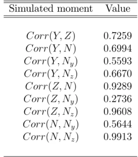
In table 4 I report simulated contemporaneous correlations for …nal output, intermediate input, aggregate employment and sector-speci…c employment. The model economy predicts a strong positive contemporaneous correlation for aggregate employment and labor input in the intermediate-good sector (0.9913). Besides, according to table 4, intermediate input and labor input in the materials sector are highly correlated (0.9608) while the correlation between …nal output and employment in the …nal-good sector is only 0.5593. Also, I should notice that …nal output is more correlated with intermediate input than with labor input in the …nal-good sector.
4.5
Data …t
Figure 5 compares the model simulated data versus the true ones. The model does a good job in replicating the data for both consumption and interest rates, while it tends to exaggerate the magnitude of the data for the in‡ation rate, the money balances and the real wage.
4.6
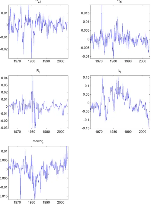
Patterns of shocks
Figure 6 shows the historical pattern of each estimated shock. While studying the shocks, it is important to keep in mind the recession dates during the Post-War period as identi…ed by the National bureau of Economic research (NBER): 1973-1974 and 1980-1981. We should note that technology shocks tend to be negative around recession dates. There are two years with the most negative shocks to technology in the two sectors: 1974 and 1980.
1980 is a year with very negative technology and monetary shocks. During the 1990’s, a period characterized by high productivity growth rates, there is no remarkable positive technology shocks. Rather, this period experienced a series of small positive and negative technology shocks.
The period 1980-1983 is marked by a succession of very negative then very positive monetary shocks.
Money-demand shocks tend to be positive between 1970 and 1990 while they become negative from 1990.
Finally, a noticeable feature of the shocks in …gure 6 is that series appear to be less volatile outside the recession periods and especially after 1982.
5
Conclusion
This paper examines whether I could reconcile with the standard RBC fric-tionless theory in terms of matching the patterns of variables in response to technology shocks, in a two-stage productive framework with both price and wage rigidities. While a positive shock to productivity in the …nal good sector leads to a persistent decrease in labor input and thus a negative corre-lation between aggregate output and labor, a positive shock to productivity in the intermediate input sector provides a good support to the RBC models predictions. In fact, it emerges from the estimation results that a positive shock to technology in the intermediate good sector produces a permanent increase in labor input in both sectors and in the aggregate labor input. Moreover, this shock explains the largest part of both aggregate output and employment ‡uctuations and thus could be considered as the driving force of the ‡uctuations in this model.
Appendix A
Steady state
Since there is no trend-growth in productivity, a steady state obtains if Ay =
Az = 1. In this steady state, the optimal pricing rules, (17), (22) and (23)
reduce to: y = y y 1 ; and z = z z 1 ; rk = 1 1 + ; R = y; Ky Y = y(1 ) rk y ; Kz Z = z rk z ; Nz Z = Az Kz Z z 1 1 z ; Ny Y = Z Y (1 y )(1 ) K y Y y y 1 ; w = (1 z) z Nz Z 1 ;
Besides, w = (1 y)(1 ) y Y Ny =) Y Ny = y z (1 z) (1 y)(1 ) Nz Z 1 ; This gives, Z Y = Ny Y (1 y )(1 ) Ky Y y (1 ) ; Pz = y Z Y 1 ; Nz Ny = Nz Z Z Y Ny Y 1 ; Ny = N 1 + Nz Ny ; Nz = N Ny; Z = Nz Nz Z 1 ; Then, Y = Z Z Y 1 ; Ky = Y Y Ky 1 ; Kz = Z Z Kz 1 ; K = Kz+ Ky I = K; C = Y I; m = Cb(1 ) = C 1 + b1m 1 :
Log-linearized system
For any variable xt, I de…ne xbt = log(xxt) as the deviation of xt from its
steady-state value. 1 ^Ct = ^t+ ^t; 1 ^bt 1 ^ mt = ^t+ ^t+ 1 R 1 R^t; ^t = ( 1)C 1 C^t+ 1b1m 1 ^bt+ 1b1m 1 m^t; ^t= ^Rt+ ^t+1 ^y;t+1; ^t+ (1 + ) ^Kt+1+ ( ) ^Kt= ^t+1+ ( rk) ^rk;t+1 ( ) bIt+1; ^w;t= bw;t+1+ (1 dw)(1 dw) dw N 1 N ^ Nt ^t w^t ; ^w;t= ^wt w^t 1+ ^y;t; ^ rk;t= ^y;t+ ^Yt K^y;t; ^ wt= ^y;t+ ^Yt [1+(1+ )'y y (1 y)(1 ) ] ^Ny;t+'y y (1 y)(1 ) [ ^Ny;t 1+ EtN^y;t+1];
^ pz;t= ^y;t+ ^Yt Z^t; ^y;t= Et^y;t+1 (1 dy)(1 dy ) dy ^y;t; ^
Yt= (1 ) ^Ay;t+ Zbt+ y(1 ) ^Ky;t+ (1 y)(1 ) ^Ny;t;
^ rk;t = ^z;t+ ^Zt K^z;t; ^ wt = ^z;t+ ^Zt [1 + 'z z 1 z (1 + )] ^Nz;t+ 'z z 1 z [ ^Nz;t 1 N^z;t+1]; ^ Zt= ^Az;t+ zK^z;t+ (1 z) ^Nz;t; ^z;t= Et^z;t+1 (1 dz)(1 dz ) dz ^z;t; ^z;t= ^pz;t p^z;t 1+ ^y;t; ^ Yt= C Y ^ Ct+ I Y ^ It; ^ Rt= % ^y;t+ %ybyt+vbt; b vt= %vvdt 1+ "R;t (33)
^ It= 1 ^Kt+1 ( 1 1) ^Kt; ^ Kt = Ky K ^ Ky;t+ Kz K ^ Kz;t; ^ Nt= Ny N ^ Ny;t+ Nz N ^ Nz;t:
References
[1] Ambler, Steven, Guay, Alain and Phaneuf, Louis. “Labor Market Im-perfections and the Dynamics of Postwar Business Cycles ”
[2] Basu, Susanto.“Intermediate Goods and Business Cycles: Implication for Productivity and Welfare.” American Economic Review 3: 512-531 (1995).
[3] Basu, Susanto.“Technology and Business Cycles: How Well Do Stan-dard Models Explain The Facts?” in "Beyond Shocks: What Causes Business Cycles?" Conferences Series No.42, Federal Reserve Bank of Boston (June 1998).
[4] Basu, Susanto; Fernald, John and Kimball, Miles.“Are Technology Im-provements Contractionary?” International Finance Discussion Papers No 625, Board of Governors of the Federal Reserve System (1998). [5] Bergin, P.R., Feenstra, R.C.“Staggered Price Setting , Translog
Prefer-ences and Endogenous Persistence.”Journal of Monetary Economics 45: 657-680 (2000).
[6] Blanchard, Olivier Jean.“Price Asynchroniszation and Price Level In-ertia.” in Dornbush , R., Simonsen, M.H. (Eds), In‡ation, Debt, and Indexation. Cambridge, Massachusetts: 3-24 (1983).
[7] Blanchard, Olivier Jean and Kahn, Charles M.“The Solution of Linear Di¤erence Equations Under Rational Expectations.” Econometrica 48: 1305-1311 (1980).
[8] Blanchard, Olivier Jean and Kiyotoki, Nobuhiro.“Monopolistic Com-petition and the E¤ects of Aggregate Demand.” American Economic Review 77: 647-666 (1987).
[9] Boudaya, Chahnez.“The E¤ects of Technological Innovations on Em-ployment: A New Explanation.”Cahiers de la MSE No.2005.13 (2005). [10] Calvo, Guillermo A.“Staggered Prices in a Utility Maximizing
[11] Carlsson, Mikael.“Measures of Technology and the Short-Run Responses to Technology Shocks: Is the RBC-Model Consistent with Swedish Man-ufacturing Data?” (2000)
[12] Chang, Yongsung and Hong, Jay H.“On the Employment E¤ect of Tech-nology: Evidence from US Manufacturing for 1958-1996.” Federal Re-serve Bank of Richmond Working Papers No 03-06 (2003).
[13] Christiano, L., Eichenbaum, M. and Vigfusson, R.“What Happens Af-ter a Technology Shock?” Board of Governors of the Federal Reserve System, International Finance Discussion Paper , 768 (2003).
[14] Cooley, Thomas F. and Gary D. Hansen. “The In‡ation Tax in a Real Business Cycle Model.” American Economic Review vol.79 No.4: 733-748 (1989).
[15] Dib, Ali and Phaneuf, Louis.“An Econometric U.S Business Cycle Model with Nominal and Real Rigidities.” CREFE, Université du Québec à Montréal, Working Paper No.137 (2001).
[16] Dotsey, Michael.“Structure from Shocks.”mimeo, Federal Reserve Bank of Richmond (1999a).
[17] Francis, Neville and Ramey, Valerie A.“Is the Technology-Driven Real Business Cycle Hypothesis Dead? Shocks and Aggregate Fluctuations Revised.” manuscript, UCSD (2001).
[18] Gali, Jordi.“Technology, Employment, and the Business Cycle:Do Tech-nology Shocks Explain Aggregate Productivity?” American Economic Review 89: 249-271 (1999).
[19] — — — — –.“New Perspectives on Monetary Policy, In‡ation and the Business Cycle.” NBER Workin Paper w8767 (February 2002).
[20] Gri¢ n, Peter.“The Impact of A¢ rmative Action on Labor Demand: A Test of Some Implications of the Le Chatelier Principle.” Review of Economics and Statistics 74: 251-260 (1992).
[21] — — — — — –.“Input Demand Elasticities for Heterogenous Labor: Firm-Level Estimates and an Investigation into the E¤ects of Aggregation.” Southern Economic Journal 62: 889-901 (1996).
[22] Hamilton, James D. “Times Series Analysis.” Princeton University Press, Princeton, New jersey (1994).
[23] Hornstein, Andreas and Praschnik, Jack.“Intermediate Inputs and sec-toral Comovement in the Business Cycle.”Federal Reserve Bank of Rich-mond Working Paper No.97-6 (1997).
[24] Huang, Kevin X.D.and Liu, Zheng.“Production Chains and General Equilibrium Aggregate Dynamics.” Journal of Monetary Economics 48:437-462 (2001).
[25] — — — — — — — — — — — — — — — .“Staggered Contracts and Business Cycle Persistence.” Institute for Empirical Macroeconomics Discussion Paper 127, Federal Reserve Bank of Minneapolis (1998).
[26] — — — — — — — — — — — — — — — .“In‡ation Targeting: What In‡ation to Target?”Federal Reserve Bank of Philadelphia Working Paper No.04-6 (July 2004).
[27] Huang, Kevin X.D.; Liu, Zheng and Phaneuf, Louis.“On the Transmis-sion of Monetary Policy Shocks”.CREFE Working Papers 112 (2000). [28] Ireland, Peter N.“ A Small, Structural, Quarterly Model for Monetary
Policy Evaluation.”Carnegie-Rochester Conference Series on Public Pol-icy 47: 83-108 (1997).
[29] Ireland, Peter N.“Interest Rates, In‡ation, and Federal Reserve Policy Since 1980.”Journal of Money, Credit and Banking 32: 417-431 (2000). [30] Ireland, Peter N.“Endogenous Money or Sticky Prices?”Journal of
Mon-etary Economics 50: 1623-1648 (2003).
[31] Jermann, Urban.“Asset Pricing in Production Economies.” Journal of Monetary Economics: 257-275 (1998).
[32] Kiley, Michael T.“Partial Adjustment and Staggered Price Setting.” Manuscript, Federal Reserve Board (1998).
[33] Kim, J.“Constructing and Estimating a Realistic Optimizing Model of Monetary Policy.” Journal of Monetary Economics 45: 329-59 (2000).
[34] King, Robert G., and Wolman, Alexander.“In‡ation Targeting in a St. Louis Model of the 21st Century.” Federal Reserve Bank of St. Louis Review 78: 83-107 (1996).
[35] Kydland, Finn and Edward Prescott. “ Time to Build and Aggregate Fluctuations.” Econometrica vol.50 No.6 (November 1982).
[36] Long, J and Plosser, C.“Real Business Cycles.”Journal of Political Eco-nomics 91: 39-69 (1983).
[37] — — — — — — — — — — -.“Sectoral vs Aggregate Shocks in the Business Cycle.”American Economics Review: Papers and Proceedings 77: 333-336 (1987).
[38] Longot, F.“Sectoral Shocks and Employment Reallocation in a Two-Sector Dynamic General Equilibrium Model.” First Version May 1997. [39] Marchetti, Domenico J. and Nucci, Francesco.“Price Stickiness and the
Contractionary E¤ect of Technology Shocks.” European Economic Re-view, forthcoming.
[40] Means, G.C.“Industrial prices and their relative in‡exibility.”U.S. Sen-ate Document 13, 74th Congress, 1st Session, Washington DC (1935). [41] Rotemberg, Julio.“Prices, Output, and Hours: An Empirical Analysis
Based on a Sticky Price Model.” Journal of Monetary Economics 37: 505-533 (1996).
[42] Shea, John.“What Do Technology Shocks Do?”NBER Working Papers 6632 (1998).
[43] Taylor John.“Discretion Versus Policy Rules in Practice.” Carnegie-Rochester Conference Series on Public Policy 39: 195-214 (1993). [44] — — — — — .“An Historical Analysis of Monetary Policy Rules.” NBER
Working Paper No.6768 (October 1998).
[45] — — — — — .“Monetary Policy Rules.” University of Chicago Press and NBER (1999).
Table 1: Maximum likelihood estimates
Parameter de…nition Parameter Estimate Std t-stat p-value Autoc. tech. …nished good sector A;y 0:8633 0:0628 13:7532 0:0000
Autoc. tech. intermediate good sector A;z 0:9900 0:0090 110:552 0:0000 Autoc. monetary policy %v 0:5545 0:0358 15:4829 0:0000 Autoc. money demand b 0:9411 0:0199 47:2776 0:0000
Autoc. measurment error merror 0:9375 0:0236 39:6937 0:0000 std. tech. …nished good sector A;y 0:0087 0:0011 7:9813 0:0000
std. tech. intermediate good sector A;z 0:0028 0:0002 12:3175 0:0000
std. monetary policy R 0:0038 0:0002 21:9383 0:0000
std. money demand b 0:1286 0:0052 24:8684 0:0000
std. measurment error merror 0:0068 0:0003 20:4247 0:0000
Policy reaction to in‡ation % 1:0074 0:0108 93:0324 0:0000 Policy reaction to output gap %y 0:0752 0:0169 4:4529 0:0000 Degree of wage stickiness dw 0:8295 0:0319 26:038 0:0000
Degree of price stick. …nal sector dy 0:4341 0:0451 9:6198 0:0000
Degree of price stick. intermediate sector dz 0:3677 0:1708 2:153 0:0401
Capital adj. cost 4:2646 0:9718 4:3884 0:0000 Labor adj. cost …nal sector 'y 0:5533 1:5379 0:3598 0:3731 Labor adj. cost intermediate sector 'z 6:4969 1:9596 3:3154 0:0019 Interm. share in …nal secor 0:2997 0:0066 45:2947 0:0000 Labor share …nal sector y 0:3025 0:0256 11:8049 0:0000
Labor share intermediate sector z 0:2567 0:0371 6:9142 0:0000
Table 2: Variance decomposition
Variable Ay;t Az;t Rt bt merrort
Yt 10:7539 54:0584 35:1816 0:0061 0:0000 Zt 15:4560 80:6244 3:9187 0:0008 0:0000 Ct 42:8075 36:8819 20:1907 0:1200 0:0000 It 4:7563 66:6808 28:5543 0:0087 0:0000 Nt 33:1152 57:4004 9:4824 0:0020 0:0000 Ny;t 7:3087 12:6376 80:0364 0:0173 0:0000 Nz;t 32:3165 50:3449 17:3349 0:0037 0:0000 wt 16:6865 78:3459 4:9659 0:0017 0:0000 Rt 1:1747 98:7156 0:1091 0:0006 0:0000 y;t 1:2056 88:3280 0:4312 0:0004 10:0349 z;t 1:3102 96:7788 1:9095 0:0014 0:0000 w;t 0:8959 99:0047 0:0991 0:0003 0:0000
Table 3: Some Second Order Unconditional Moments Moments Post-war US data Model prediction
std(Y ) 0:0170 (0:0023) 0:0260 std(C) 0:0123 (0:0017) 0:0121 std(I) 0:0509 (0:0073) 0:0523 std(N ) 0:0042(0:0003) 0:0395(0:0080) 0:0480 std(w) 0:0110 (0:0026) 0:0218 Corr(Y; C) 0:9305 (0:2526) 0:3295 Corr(Y; I) 0:8908 (0:2374) 0:9698 Corr(Y; w) 0:7399 (0:3696) 0:5277 Corr(Y; N ) 0:6813(0:1548) 0:0880(1:1121) 0:6994 Corr(N; w) 0:4442(0:1652) 0:0559(2:2928) 0:2057
Table 4: Sectoral Comovements Simulated moment Value
Corr(Y; Z) 0:7259 Corr(Y; N ) 0:6994 Corr(Y; Ny) 0:5593 Corr(Y; Nz) 0:6670 Corr(Z; N ) 0:9289 Corr(Z; Ny) 0:2736 Corr(Z; Nz) 0:9608 Corr(N; Ny) 0:5644 Corr(N; Nz) 0:9913