HAL Id: hal-01890473
https://hal-centralesupelec.archives-ouvertes.fr/hal-01890473
Submitted on 8 Oct 2018
HAL is a multi-disciplinary open access
archive for the deposit and dissemination of
sci-entific research documents, whether they are
pub-lished or not. The documents may come from
teaching and research institutions in France or
abroad, or from public or private research centers.
L’archive ouverte pluridisciplinaire HAL, est
destinée au dépôt et à la diffusion de documents
scientifiques de niveau recherche, publiés ou non,
émanant des établissements d’enseignement et de
recherche français ou étrangers, des laboratoires
publics ou privés.
A New Qualitative Language for Qualitative Simulation
Slim Medimegh, Jean-Yves Pierron, Frédéric Boulanger
To cite this version:
Slim Medimegh, Jean-Yves Pierron, Frédéric Boulanger. A New Qualitative Language for
Qualita-tive Simulation. International Symposium on Computer Science and Intelligent Control, Sep 2018,
Stockholm, Sweden. �hal-01890473�
Slim Medimegh
CEA LIST, Laboratory of Model Driven Engineering for Embedded
Systems France [email protected]
Jean-Yves Pierron
CEA LIST, Laboratory of Model Driven Engineering for Embedded
Systems France
Frédéric Boulanger
LRI, CentraleSupélec, Université Paris-Saclay
France
ABSTRACT
Cyber physical systems are specified in a hybrid form, with discrete and continuous parts. Simulating such systems requires precise data and synchronization of continuous changes and discrete transitions. However, in the first design steps, missing information forbids nu-merical simulation. We present here a new qualitative language for qualitative simulation of cyber physical systems, which con-sists in computing the relationships between the system variables. This language is implemented in the Diversity symbolic execution engine to build the traces of the system. We apply this approach to the analysis of SysML models, using an M2M transformation from SysML to a pivot language, an M2T transformation from this language to Diversity and an analysis of the traces obtained by Diversity to build the qualitative behaviors of the system.
KEYWORDS
Cyber physical systems, qualitative simulation, symbolic execution, model transformation, qualitative behavior
ACM Reference Format:
Slim Medimegh, Jean-Yves Pierron, and Frédéric Boulanger. 2018. A New Qualitative language for Qualitative Simulation. In Proceedings of ACM Conference (Conference’17). ACM, New York, NY, USA, 10 pages. https: //doi.org/10.1145/nnnnnnn.nnnnnnn
1
INTRODUCTION
Embedded systems have become crucial in the industry, and their design leads to hybrid models of a whole system, which mix discrete and continuous parts. Simulating such complex systems requires precise data and computational power for detecting changes in the continuous values and synchronizing them with discrete transitions. However, in the early steps of the design, the numerical value of some parameters is not known yet, while it is already necessary to analyze the behavior of the system to make design decisions.
For continuous variables, the evolution laws are often described by differential equations. Qualitative simulation can be an alterna-tive to numerical simulation for this kind of models to compute the qualitative behaviors of the system.
Its principle is the discretization of the domain of variation of the continuous variables, their derivatives and second derivatives, leading to a qualitative representation of their evolution: positive, negative, null, increasing, decreasing, constant, at a minimum etc. In this way, one can get a tree of abstract behaviors, each node describing the qualitative evolution of the variables. Combined with a model of the discrete part of the system, a discrete model of the behavior of the whole system is established, to which formal techniques can be applied.
However, sometimes the differential equations are not available, or some constants are not known yet. In this case, we can use an abstract model of the laws of evolution of the variables to perform the qualitative simulation. This qualitative model captures the vari-ations of continuous variables and their causal links. For instance, precise values and differential equations are not necessary to pre-dict that an object dropped in a gravitational field will fall down. Such a qualitative model of a continuous behavior can be described by an automata as discussed later.
In this article, we present a new language for qualitative simu-lation without differential equations, which relies on a qualitative constraint model describing the relationships between the system variables. This model of constraint is implemented in the Diver-sity [8] [15] tool in order to compute the qualitative traces of cyber physical systems.
We designed a profile for SysML to model our qualitative con-straints, and use model driven engineering techniques such as QVTop [6] and Acceleo [5] in order to have a complete tool chain that takes a SysML model and produces a Diversity model. We add an analysis module in our tool chain to extract the qualitative behaviors of the systems from Diversity traces.
This article has two main parts: in the first one, we present the context of our work and our constraint execution model for quali-tative simulation, in the second part we present how we designed the profile for SysML in this context.
2
QUALITATIVE SIMULATION OF CYBER
PHYSICAL SYSTEMS
Cyber physical systems consist of continuous dynamic systems, discrete event systems and an interface that handles the interac-tion between both types of systems [12]. Such systems result from the hierarchical organization of monitoring/control systems, or from the interaction between algorithms for discrete planning and continuous control. These systems can be modeled using hybrid automata, which are defined by a set of continuous variables and states, and discrete transitions with guards and assignments to these variables.
Qualitative simulation comes from artificial intelligence, where it is used for reasoning about continuous aspects of systems. The goal is to reason about the behavior of a continuous variable without computing its value.
For Cyber physical systems, the model of the discrete part of the system is not influenced by the qualitative abstraction process. However, continuous variables and their derivatives are discretized in order to consider only their qualitative changes. Therefore, con-tinuous behaviors become discrete transitions, and the resulting
system is entirely discrete and can be treated by traditional methods for the verification of discrete systems.
2.1
Principle of Qualitative Simulation
Qualitative simulation is based on the principle of discretization by partitioning the variation range of the continuous variables of the system and their derivative to compute their qualitative state (in-creasing, de(in-creasing, constant etc.) This principle can be extended
to the nthderivative to distinguish more qualitative states. Once
the discrete states corresponding to this qualitative partitioning are created, we build the possible transitions between them by taking into account continuity and derivative constraints. For instance, each variable or derivative can not go from negative to positive without going through zero, and a variable can go from negative to zero or from zero to positive only if its derivative is positive etc. This limits the possibilities of evolution and thus reduces the size of the corresponding automaton. Finally, the differential equation sys-tem is abstracted into a transition syssys-tem whose states are based on the partitioning of the changes of continuous variables and deriva-tives, and whose transitions are the physically possible evolutions between these states. The result of the qualitative simulation is an abstraction of the solutions to the differential equations system.
2.2
Types of Qualitative Simulation
Qualitative Simulation can be used according to two strategies [9]: qualitative simulation with differential equations, and qualitative simulation without differential equations. In the first approach, the differential equations are known, and tools like QEPCAD [3] are used to determine the conditions for a qualitative change. When a change is possible, the corresponding branch in the execution tree is tagged with the conditions, else it is cut.
In the second approach, the differential equations are not avail-able (some constants are not known yet) or it is too difficult to deal with their complexity. In this case, we build a qualitative model of the equations by considering qualitative relations between the variables and their derivatives. Of course, the results are less precise than with the first approach, but this can be used at the first steps of the design. In this article, we deal with the second approach. We therefore use Diversity, which is a symbolic execution tool, to compute the qualitative behaviors of the model of a cyber physical system, combining the model of its discrete part and the discretized qualitative model of its continuous part.
2.3
Qualitative behaviors
The result obtained from qualitative simulation is a set of qualita-tive behaviors. Each qualitaqualita-tive behavior is an equivalence class representing detailed behaviors of the system and is composed of a set of qualitative contexts. As illustrated in Figure 1 a qualitative context includes : (1) a Control State (CS), here it corresponds to
the state where both variablesx and y have a null derivative; (2) a
Path Condition (PC), which is the condition to reach the symbolic state from the initial state, here, both Ûx♯1and Ûy♯1are null; (3) a symbolic memory which associates to each variable an expression based on symbolic inputs. The ♯ notation is used to index successive symbolic values. EC = CS : Null_der_x , Null_der_y PC : Ûx♯1= 0, Ûy♯1= 0 Ü x-1= Üx-1♯0, Üy-1= Üy-1♯0 Û x = Ûx♯1, Ûy = Ûy♯1
Figure 1: Execution Context
2.4
Related Work
Kuipers’ algorithm, which is the first contribution to qualitative simulation, and is implemented in QSIM [10], is based on an algebra of signs (negative, positive, null). Numerous improvements have been added to QSIM in order to address the combinatory explosion of the number of predicted states caused by the addition of two entities with opposite sign :
• Methods for changing the level of description to add addi-tional information in order to eliminate behaviors with no qualitative distinctions [11].
• Reasoning on “high order derivative” to provide curvature constraints [11] [4].
• Adding energy constraint that decomposes the system into a conservative part and a non conservative one [7]. The most famous tool for qualitative simulation is Garp3 [2]. It runs model fragments, which describe part of the structure and behavior of the system, and produces a state graph which contains all the possible transitions based on the relationships between entities that are described in the model fragments. Garp3 provides a language based on two principle operators : proportionality and influence. Proportionality deals with the derivatives of the variables: P+(Q2, Q1) causes Q2 to increase if Q1 increases and to decrease if Q1 decreases. Influence deals with the value and the derivative: I+(Q2, Q1) causes Q2 to increase if Q1 is > 0, and to decrease if Q1 is < 0. Here, we notice that there is a lack of expressiveness, for example, we can not model with these two operators the relationship between a second derivative and a value, for example we can not model
that the weightp of an object is the product of its mass m by the
gravitational accelerationд (p = mд). Also, we need to add multiple
thresholds to the operators besides the default ones which are 0, when the user is interested in some critical values other than 0.
Garp3 provides a state graph as a result of the qualitative simula-tion. This state graph describes all the possible qualitative behaviors of the system with all the variables included. However, sometimes the user want to ignore some variables and see the impact on the qualitative behaviors obtained. We therefore provide an incremen-tal methodology allowing us to select the variables that we want to observe in order to establish the qualitative behaviors on.
In [14], Missier and Trave-Massuyes proposed a temporal filter based on order of magnitude representation and second order Taylor formula to evaluate the duration for qualitative states, in our case we are not interested in temporal information because we are in the first steps of the design; time is not critical at this stage. We therefore propose a new qualitative language based on a constraint qualitative model to enable the expression of multi level coupled variables with different thresholds representing the critical landmarks from a user point of view.
2.5
A new Constraint Execution Model for
Qualitative Simulation
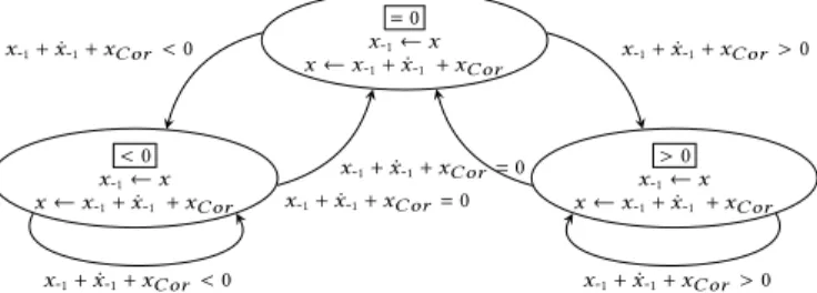
For improving the qualitative simulation without differential equa-tions in Diversity, we developed a model of execution that con-straints the evolution of the state variables, and computes their qualitative behavior = 0 x-1←x x ← x-1+ Ûx-1 < 0 x-1←x x ← x-1+ Ûx-1 > 0 x-1←x x ← x-1+ Ûx-1 Û x-1< 0 xÛ-1> 0 Û x-1> 0and Û x-1= −x Û x-1< 0and Û x-1= −x ( Ûx-1< 0)or ( Ûx-1> 0andxÛ-1< −x) ( Ûx-1> 0)or ( Ûx-1< 0andxÛ-1> −x)
Figure 2: Qualitative changes based on symbolic integration
2.5.1 Model Of Execution. In our previous work [13] we
pre-sented a symbolic execution model in which we integrate the deriva-tives of the state variables in a symbolic way. We use a simple Euler integration since we do not compute exact numerical values. We model each continuous state variable by six values: the current
(x) and previous (x-1) values of the variable, the current ( Ûx) and
previous ( Ûx-1) values of its first derivative, and its current second
derivative ( Üx). In this new model of execution, we add the previous
second derivative ( Üx-1), which is needed to integrate the first
deriv-ative. The symbolic integration with the Euler method, assuming a unitary integration step givesx = x-1+ Ûx-1, and Ûx = Ûx-1+ Üx-1.
With these rules, the qualitative value of a state variable is con-trolled by a state machine as illustrated in Figure 2. A similar au-tomaton controls the change of the first derivative with respect to its previous value ( Ûx-1) and the previous second derivative ( Üx-1).
Contrary to our previous work, these state machines are determin-istic. For instance, in the > 0 state ofx, if Ûx-1< 0 and Ûx-1= -x-1, we
go to the= 0 state, if Ûx-1> 0 or Ûx-1< 0 and - Ûx-1<x, we stay in the
current state.
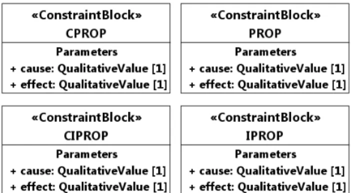
In this paper, we present a constraint qualitative model in which we link the derivatives and the values of two state variables. We define four operators inspired from [2]:
• causally proportional : CPROP • proportional : PROP
• causally inversely proportional : CIPROP • inversely proportional : IPROP
We will use thres to give the threshold of the state variables.
2.5.2 CPROP. This operator models the causal proportionality
between the values of two different state variables. For example,x
thresTc is CPROPy thres Tsmeans that the sign ofx −Tchas
to be the same as the sign ofy − Ts, but a correction tox will be
made only when we detect a change of sign ofy −Ts. So, ify-1= Ts,
y > Ts andx = Tc, we have to make the value ofx > Tc. However,
ifx goes below Tcwhiley remains above Ts, we won’t try to fixx.
Compared to our previous work [13], where we hadx = x-1+ Ûx-1,
we need to add a corrective termxCor to fix the value ofx when
necessary. As a resultx = x-1+ Ûx-1 + xCor.
2.5.3 PROP. This operator models the proportionality between
the value of two different state variables. For example, Ûx thres 0
is PROP Ûy thres 0 means that the sign of Ûx and the sign of Ûy
have to be the same. Contrarily to CPROP, a qualitative change
in Ûy is not necessary to enforce the proportionality. Compared to
our previous work [13], where we had Ûx = Ûx-1+ Üx-1, we need to
add a corrective term ÛxCor to Ûx in order to fix the value of Ûx when
necessary. As a result Ûx = Ûx-1+ Üx-1 + ÛxCor.
2.5.4 CIPROP. This operator models the inverse proportionality
between the values of two different state variables. For example, Ü
x thres 0 is CPROP y thres Tsmeans that the signs of Üx and
y − Ts have to be opposite, but a correction is enforced only when
we detect a qualitative change iny − Ts. Ify-1 = Ts,y > Ts and
Ü
x ≥ 0, we have to fix the value of Üx to make it negative. Compared
to our previous work [13], where we had Üx = Üx-1, we need to add
a corrective term ÜxCor to Üx in order to fix the value of Üx when
necessary. As a result Üx = Üx-1 + ÜxCor.
2.5.5 IPROP. This operator models the inverse proportionality
between the values of two different state variables. For example, Ûx
thres 0 is IPROP Ûy thres 0 means that the sign of Ûx and the sign
of Ûy have to be opposite, and the correction on Ûx must be performed
even without a qualitative change in Ûy. If Ûy < 0 and Ûx ≥ 0, we have
to fix the value of Ûx to make it negative. Compared to our previous
work [13] where we had Ûx = Ûx-1+ Üx-1, we need to add a corrective
term ÛxCorto Ûx in order to fix the value of Ûx when necessary. As a
result Ûx = Ûx-1+ Üx-1 + ÛxCor. = 0 x-1←x x ← x-1+ Ûx-1+ xC or < 0 x-1←x x ← x-1+ Ûx-1+ xC or > 0 x-1←x x ← x-1+ Ûx-1+ xC or x-1+ Ûx-1+ xC or < 0 x-1+ Ûx-1+ xC or> 0 x-1+ Ûx-1+ xC or= 0 x-1+ Ûx-1+ xC or= 0 x-1+ Ûx-1+ xC or< 0 x-1+ Ûx-1+ xC or> 0
Figure 3: Qualitative changes based on qualitative con-straints
With these rules, the qualitative value of a state variable is
con-trolled by a state machine. If we consider for examplex thres 0
is CPROP y thres 0, the corrective term xCor will be added in
the symbolic integration ofx as illustrated in Figure 3. For instance,
in the= 0 state of x, if x-1+ Ûx-1 + xCor > 0, we go to the > 0
state, ifx-1+ Ûx-1 + xCor < 0, we go to the < 0 state. A similar
automaton controls the change of the first derivative with respect to its previous value ( Ûx-1), the previous second derivative ( Üx-1) and
the corrective terms from the different relations that are linked to the first derivative.
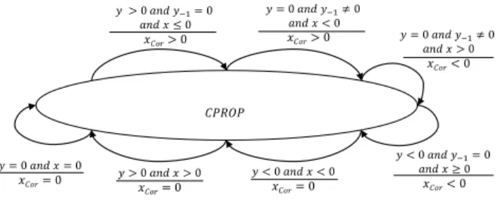
2.5.6 Implementation of the Generation of the Corrective Term.
The generation of the corrective terms is controlled by a state machine. The goal of the corrective term is to change the variable
𝐶𝑃𝑅𝑂𝑃 𝑦 > 0 𝑎𝑛𝑑 𝑦−1= 0 𝑎𝑛𝑑 𝑥 ≤ 0 𝑥𝐶𝑜𝑟> 0 𝑦 = 0 𝑎𝑛𝑑 𝑦−1≠ 0 𝑎𝑛𝑑 𝑥 < 0 𝑥𝐶𝑜𝑟> 0 𝑦 = 0 𝑎𝑛𝑑 𝑦−1≠ 0 𝑎𝑛𝑑 𝑥 > 0 𝑥𝐶𝑜𝑟< 0 𝑦 < 0 𝑎𝑛𝑑 𝑦−1= 0 𝑎𝑛𝑑 𝑥 ≥ 0 𝑥𝐶𝑜𝑟< 0 𝑦 > 0 𝑎𝑛𝑑 𝑥 > 0 𝑥𝐶𝑜𝑟= 0 𝑦 < 0 𝑎𝑛𝑑 𝑥 < 0 𝑥𝐶𝑜𝑟= 0 𝑦 = 0 𝑎𝑛𝑑 𝑥 = 0 𝑥𝐶𝑜𝑟= 0
Figure 4: Qualitative automaton of the CPROP operator
𝑃𝑅𝑂𝑃 𝑦 > 0 𝑎𝑛𝑑 𝑥 ≤ 0 𝑥𝐶𝑜𝑟> 0 𝑦 = 0 𝑎𝑛𝑑 𝑥 < 0 𝑥𝐶𝑜𝑟> 0 𝑦 = 0 𝑎𝑛𝑑 𝑥 > 0 𝑥𝐶𝑜𝑟< 0 𝑦 < 0 𝑎𝑛𝑑 𝑥 ≥ 0 𝑥𝐶𝑜𝑟< 0 𝑦 > 0 𝑎𝑛𝑑 𝑥 > 0 𝑥𝐶𝑜𝑟= 0 𝑦 < 0 𝑎𝑛𝑑 𝑥 < 0 𝑥𝐶𝑜𝑟= 0 𝑦 = 0 𝑎𝑛𝑑 𝑥 = 0 𝑥𝐶𝑜𝑟= 0
Figure 5: Qualitative automaton of the PROP operator
𝐶𝐼𝑃𝑅𝑂𝑃 𝑦 > 0 𝑎𝑛𝑑 𝑦−1= 0 𝑎𝑛𝑑 𝑥 ≥ 0 𝑥𝐶𝑜𝑟< 0 𝑦 = 0 𝑎𝑛𝑑 𝑦−1≠ 0 𝑎𝑛𝑑 𝑥 < 0 𝑥𝐶𝑜𝑟> 0 𝑦 = 0 𝑎𝑛𝑑 𝑦−1≠ 0 𝑎𝑛𝑑 𝑥 > 0 𝑥𝐶𝑜𝑟< 0 𝑦 < 0 𝑎𝑛𝑑 𝑦−1= 0 𝑎𝑛𝑑 𝑥 ≤ 0 𝑥𝐶𝑜𝑟> 0 𝑦 > 0 𝑎𝑛𝑑 𝑥 < 0 𝑥𝐶𝑜𝑟= 0 𝑦 < 0 𝑎𝑛𝑑 𝑥 > 0 𝑥𝐶𝑜𝑟= 0 𝑦 = 0 𝑎𝑛𝑑 𝑥 = 0 𝑥𝐶𝑜𝑟= 0
Figure 6: Qualitative automaton of the CIPROP operator
𝐼𝑃𝑅𝑂𝑃 𝑦 > 0 𝑎𝑛𝑑 𝑥 ≥ 0 𝑥𝐶𝑜𝑟< 0 𝑦 = 0 𝑎𝑛𝑑 𝑥 < 0 𝑥𝐶𝑜𝑟> 0 𝑦 = 0 𝑎𝑛𝑑 𝑥 > 0 𝑥𝐶𝑜𝑟< 0 𝑦 < 0 𝑎𝑛𝑑 𝑥 ≤ 0 𝑥𝐶𝑜𝑟> 0 𝑦 > 0 𝑎𝑛𝑑 𝑥 < 0 𝑥𝐶𝑜𝑟= 0 𝑦 < 0 𝑎𝑛𝑑 𝑥 > 0 𝑥𝐶𝑜𝑟= 0 𝑦 = 0 𝑎𝑛𝑑 𝑥 = 0 𝑥𝐶𝑜𝑟= 0
Figure 7: Qualitative automaton of the IPROP operator
on the left side of the relation (the affected variable) in a way to make the relation true. For causal relation, the corrective term is set only when the relation becomes false because of a change in the variable on the right side of the relation (the cause variable). For
instance, let us considerx thres 0 is CPROP y thres 0. This
relation is modeled by an automaton as illustrated in Figure 4. As shown in this figure, we wait for the qualitative change of the cause variable of the relation (y) in order to set a new qualitative value
for the corrective term. Wheny becomes > 0 and x ≤ 0, we need
to set a new > 0 qualitative value to the corrective term in order to
make the symbolic value ofx positive. Of course, when the value of
x and y are proportional again, we need to set back the qualitative value of the corrective term to 0.
Let us now considerx thres 0 is PROP y thres 0. This relation
is modeled by an automaton as illustrated in Figure 5. As shown in this figure, we do not wait for the qualitative change of the cause variable of the relation(y) in order to set a new qualitative value
for the corrective term. Wheny > 0 and x ≤ 0, we need to set a
new > 0 qualitative value for the corrective term in order to make
the symbolic value ofx evolve toward a positive value. Of course,
when the value ofx and y are proportional again, we need to adjust
the qualitative value of the corrective term to 0.
For the two other operator CIPROP as illustrated in Figure 6 and IPROP as illustrated in Figure 7, the automaton that sets the new qualitative value of the corrective term is very similar to the automata of CPROP and PROP except that they try to make the
qualitative values ofx and y opposite.
𝑉𝑒𝑟𝑖𝑓𝑖𝑐𝑎𝑡𝑖𝑜𝑛_𝑃𝑅𝑂𝑃 𝑁𝑜𝑡_𝑉𝑒𝑟𝑖𝑓𝑖𝑐𝑎𝑡𝑖𝑜𝑛_𝑃𝑅𝑂𝑃 𝑖𝑛 𝑜𝑡ℎ𝑒𝑟 𝑐𝑎𝑠𝑒𝑠 𝑦 = 0 𝑎𝑛𝑑 𝑥 = 0 𝑜𝑟 𝑦 > 0 𝑎𝑛𝑑 𝑥 > 0 𝑜𝑟 (𝑦 < 0 𝑎𝑛𝑑 𝑥 < 0) 𝑦 = 0 𝑎𝑛𝑑 𝑥 = 0 𝑜𝑟 𝑦 > 0 𝑎𝑛𝑑 𝑥 > 0 𝑜𝑟 (𝑦 < 0 𝑎𝑛𝑑 𝑥 < 0) 𝑖𝑛 𝑜𝑡ℎ𝑒𝑟 𝑐𝑎𝑠𝑒𝑠
Figure 8: Verification automaton of the PROP operator
2.5.7 Verification of the Relations. It is very important to know
that our Constraint Qualitative Model is based on symbolic inte-gration. So, when we set a corrective term in the execution model to bring back the affected variable of a relation to follow the cause variable, we are not sure that the relation is verified at the end of
the execution. For instance, if we considerx thres 0 is PROP y
thres 0. Wheny > 0 and x < 0, the corrective term is > 0 and
x = x-1+ Ûx-1+ xCor. Howeverx-1+ Ûx-1< 0 and xCor > 0, so x may
become > 0 or may stay ≤ 0. In the symbolic execution, we will
have these two paths. In order to tag the path in whichx > 0, we
use an automaton that observes the qualitative changes ofx with
respect to the relation, and tags the path in which the relation is verified, as illustrated in Figure 8. This automaton shows that if
the value ofx and y are proportional (they are both = 0, > 0 or
< 0), we are in a state in which the relation PROP is verified. In all the other cases, we are in a state in which the relation PROP is not verified. A quite similar automaton controls the verification of the CPROP operator but in this case it takes into consideration the qualitative changes of the cause variable of the relation. For the two other operators IPROP and CIPROP, we have two other automata for verifying that the variables linked by the relations are inversely proportional. These two automata are based on the same principle that we have discussed before for the PROP and CPROP operators.
2.5.8 Implementation of the Qualitative Constraint Model. This
execution model with qualitative constraints relies on several au-tomata: the first one is the scenario automaton in which the user specifies the behavior of the system input and specifies the different
values of the current second derivative; the second automaton calcu-lates the corrective term of the relations that model the interactions between the different state variables of the system, we have in fact as many automata calculating the corrective terms as there are relations; the third automaton keeps track of the qualitative value
of the second derivative ( Üx), which is symbolically integrated from
the previous second derivatives and the corrective terms linked to the second derivative; the fourth automaton keeps track of the
qualitative value of the first derivative ( Ûx), which is symbolically
integrated from the previous first, second derivatives and the cor-rective terms linked to the first derivative; the fifth automaton keeps track of the qualitative value of the state variable (x), which is symbolically integrated from the previous value, first derivative and the corrective terms linked to the value; the sixth automaton computes the qualitative variation of the variable by observing the automata for the qualitative value of the variable, its derivatives, and their previous value in order to detect the different qualitative variation of the state variables (Constant, Increase...) as we have shown in our previous work [13]; the seventh automata computes the verification of the relations after setting the corrective term in the model execution; and finally, the eighth automaton models the controller specified by the user. This final automata observes the outputs of the qualitative Constraints Model and try to adjust the concerned state variables for the regulation of the system.
The order in which these automata are executed is important: we execute the automaton of the scenario first, then the automata of the relations, then the automaton for the second derivative, then the automaton for the first derivative, then the automaton for the value of the state variable, then the automaton for the qualitative behavior, then the automata of the verification of the relations and finally the automaton of the controller.
2.5.9 Qualitative Behavior Analysis. Our Constraints Qualitative
Model is executed in Diversity [1] which is a symbolic execution engine developed at CEA LIST to produce symbolic scenarios corre-sponding to classes of system behaviors. Properties can be proved on this set of scenarios and concrete numerical tests can be gener-ated from them. To guarantee termination or to limit the number of generated test cases, the size and the number of behaviors can be bounded, and redundant behavior detection can be used.
There are some traces found by Diversity that differ by a few sequences of states. This is due to the way Diversity detects Redun-dancy. During the symbolic execution of a model, Diversity builds a tree, each branch corresponding to a choice for the symbolic value of the variables. When Diversity finds an execution context that was met before, it cuts the execution of this branch, and makes it point to the state that was met before. This turns the tree into an execution graph, and makes it possible to capture infinite behaviors in a finite structure. However, depending on the order in which the variables change, the redundancy detection can be delayed, which creates several execution paths for the same physical behavior.
Diversity generates also traces that include all the possible paths from our Constraints Qualitative Model. Among these traces there are paths in which the relations are not verified. These traces need to be eliminated because they do not respect the relations that model the link between the different state variables of the systems.
That is why we need to filter the results of Diversity in order to keep only one path for each possible physical behavior which represents a real qualitative behavior of the cyber physical system. For that, our tool chain that we are going to present later, includes a module which filter the basic traces of Diversity and produces the real qualitative behaviors of the system depending on the variables that we want to observe on the simulation.
Figure 9: The Tool Chain
3
A SYSML PROFILE
FOR QUALITATIVE SIMULATION
To make our approach usable by system designers, and to insulate them from changes in our execution model and input format, we have designed a profile for SysML as input language for qualitative simulation without differential equations. This makes the qualita-tive modeling of cyber physical systems in SysML easier and more expressive. We choose SysML because it allows the modeling of multi domain specifications. It is also used by a large community of engineers to model the system at the early design stages.
3.1
Presentation of the tool chain
We model a cyber physical system with a SysML model, on which we have applied our Qualitative Simulation Profile, using the Pa-pyrus Eclipse plug-in. Then, we transform the SysML model using a QVT operational “model to model” transformation into a HyDiv model. HyDiv is a pivot meta-model that we designed to capture a high level representation of the cyber physical system, indepen-dently of the source model (we could use Simulink/Stateflow instead of SysML). We then use an Acceleo model to text transformation to transform the HyDiv model into Xlia, the input language of Diversity. In order to generate the qualitative behaviors, we add an analysis trace module that takes the basic traces generated by Diversity and applies some filters to eliminate the traces that we discussed above in Qualitative Behavior Analysis as shown in Figure 9. Compared to our previous work [13], we add the relation between variables, the Qualitative Simulation Profile for SysML and the trace analysis module. Also, we have updated the HyDiv model to support the relations between the states variables of the system.
Figure 10: The Block Extension
3.2
The Qualitative Simulation Profile
Block Extension. In order to distinguish the different components of the system that we want to model in a qualitative way, we cre-ate three stereotypes; the Qualitative System to label the global system, the Qualitative Block to label the different component of the system and the Scenario to label the input component of the system as shown in Figure 10. A Qualitative system is composed of different Qualitative Block and a Scenario.
Figure 11: The State Machine Extension
State Machine Extension. In order to distinguish the different state machines that models the behavior of the system and the input of the system, we create two stereotypes; the ScenarioStateMa-chine to label the state maScenarioStateMa-chine that models the behavior of the Scenario Block; the SystemStateMachine to label the state ma-chine that models the behavior of Qualitative System as illustrated in Figure 11. The Classifier Behavior of the Qualitative System is a state machine that is tagged with the SystemStateMachine stereo-type. We do the same for the Scenario, but in this case the classifier behavior is a state machine that is tagged with the ScenarioStateMa-chine stereotype.
Figure 12: The Property Extension
Figure 13: The Qualitative Types
Property Extension. In order to distinguish the different state variables of a Qualitative block, we create the QualitativeState-Variable stereotype which is composed of three attributes as shown in Figure 12;
• order to know the order of the state variables. The order
is either first if we use only the first derivative of the state variable, or second, if we also use the second derivative of the state variable.
• threshold to know the different thresholds for the value of
the state variable.
• isContinuous to know if the value that is specified in the
order attribute is continuous or not.
A Qualitative Block contains different attributes tagged with the QualitativeStateVariable stereotype to precise the properties that our Constraint Model needs to configure the simulation. These attributes will have a Qualitative Type as type in order to use the different levels of description of a state variable as illustrated in Figure 13.
Figure 14: The Constraint Property Extension
Figure 15: The Qualitative Constraints library Constraint Block Extension. To express the continuous behav-ior of the cyber physical system in SysML, the designers use the parametric diagram. This type of diagram is used to model an equation using the Constraint Block component of SysML. In our case, we do not have the exact numerical equations, we have a qualitative model of the equations which is described by rela-tions based on the different operators of our Constraint Model explained earlier in subsection 2.5. In order to make qualitative modeling without differential equations easier in SysML, we create the QualitativeConstraintProperty stereotype that will allow us to enter easily the threshold of the linked state variables as shown in Figure 14. The QualitativeConstraintProperty has two attributes;
CauseThres, which is the threshold of the cause variable of the relation, and effectThres, which is the threshold of the affected variable of the relation. Also, we create a Qualitative Constraints Library that contains the four operators of our Constraint Model : CPROP, PROP, CIPROP and IPROP. Every operator has two at-tributes; cause and effect in order to specify the different variables of the relation as illustrated in Figure 15.
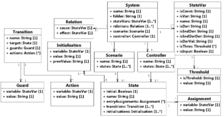
Figure 16: The HyDiv Meta Model
3.3
HyDiv Model
HyDiv is a textual domain specific modeling language for Cyber physical systems, implemented with Xtext. It provides us with a compact representation of the system which is decoupled from both the input formalism (SysML in this article) and the model of execution that will be used in Diversity. Figure 16 shows its meta-model. Compared to our previous work in [13], we add:
Relation a class to model relations between the state variables, in which we find the cause and the affected variables of the relation.
Threshold a class to model the threshold of state variables. Scenario a class in which the user specifies the behavior of
the input scenario.
Controller a class in which the user specifies the behavior of the control part of the system.
3.4
Trace analysis module
The trace analysis module is a Java application that takes the basic traces generated by Diversity as input and produces the qualitative behaviors of the cyber physical systems as output by applying some filters:
Mathematical filter eliminates the paths that end with a state variable over its threshold while its first and second deriva-tives are negative. This corresponds to an increasingly de-creasing variable that stays indefinitely above a finite thresh-old, which is mathematically impossible. The filter also elim-inates the dual case of an increasingly increasing variable which stays forever below a finite threshold (value under the threshold, positive first and second derivatives).
Validation filter eliminates the paths that end with at least one unsatisfied relation between state variables.
Observable Variable filter merges the behaviors that are sim-ilar when we hide the variables that the user did not select for observation. The detailed behaviors are still available for
inspection if the user wants to understand why we obtain these qualitative behaviors when observing only this set of variables.
Figure 17: General Principle of the Cooling System
4
USE CASE: COOLING SYSTEM
We applied our method to the cooling system shown in Figure 17. The cooling system is a basic system found in French nuclear power plants, which is used to provide cooling of auxiliary secondary cir-cuits connected to the turbine process. This is a device for cooling several hot sources through an interface with a cold source, con-trolled by exchangers. It contains logical and analog parts. In this system, we have a Heat flow that enters from the Heat source component and tries to be cooled when it goes to the Cooling component. The Heat source produces a hot temperature Thot as output while the Cooling component produces a cold temperature Tcold as output. The main goal of this system is to regulate the Tcold temperature to be equal to a set temperature Tc. For that, we have to regulate the Rate of the cold water. Four state variables in the Cooling model were the primary subject of the simulation process study: the Heat (input for the Cooling system), the hot tem-perature of the circuit (input to exchangers), the cold temtem-perature (output from exchangers) and the flow in the exchangers (given by the rate of the flow within an exchanger). All other parameters were assumed to be constant. In this system, we do not have the exact differential equations, we know only a qualitative model of these equations which could be modeled by our language in the form of relations:
• relation 1: ÛThot thres 0 is CPROP ÛHeat thres 0
• relation 2: ÛTcold thres 0 is PROP ÛThot thres 0
• relation 3: ÛThot thres 0 is PROP ÛTcold thres 0
• relation 4: ÜTcold thres 0 is CIPROP ÛRate thres 0
Relation 1 models the fact that the variation of theHeat impacts
the variation of the hot temperatureThot in a proportional way.
We want to fix the temperature only whenHeat changes, so we
use the CPROP operator. Relations 2 and 3 model the fact that
the hot temperatureThot and the cold temperature Tcold vary in
a proportional way. We want to keep this relation all the time, so
we use the PROP operator. The hot temperatureThot and the cold
temperatureTcold influence each other in a acausal way, and we
model this mutual influence by two relations; in relation 2, the
vari-ation ofThot impacts the variation of Tcold, and in relation 3, the
variation ofTcold impacts the variation of Thot. Relation 4 models
the fact that the qualitative change of the variation of theRate
Figure 18: Block Definition Diagram of the Cooling System
in a opposite way. When theRate of the cold water increases, the
cold temperatureTcold has a tendency to decrease, so the second
derivative ÜTcold is negative. When the Rate of the cold water
de-creases, the cold temperatureTcold has a tendency to increase, and
the second derivative of ÜTcold is positive.
4.1
SysML Model of the Cooling System
4.1.1 Architecture of the Cooling System. The architecture of
the cooling system is modeled in a Block Definition Diagram in SysML as shown in Figure 18. The cooling system which is a Qual-itativeSystem is composed of three QualitativeBlock: the Heat-Source block that contains a QualitativeStateVariable: Heat, the Cooling block that contains two QualitativeStateVariable: Thot and Tcold, the Regulation block that contains a QualitativeStat-eVariable: Rate and finally the Scenario block that contains the ScenarioStateMachine that specifies the variation of the Heat which is the input of the cooling system.
«SystemStateMachine» System_State_Machine Constant_Rate /entry Rate.derivative == 0 Init_System /Tcold.value == Tc t0 Increase_Rate /entry Rate.derivative > 0 t4 [Tcold.value > Tc] t5 [Tcold.value == Tc] t6 [Tcold.value > Tc] Decrease_Rate /entry Rate.derivative < 0 t1 [Tcold.value < Tc] t2 [Tcold.value == Tc] t3 [Tcold.value < Tc]
Figure 19: Regulation State Machine of the Cooling System
4.1.2 Regulation of the Cooling system. The regulation of the
cooling system is modeled by a state machine as illustrated in Figure 19 with 4 states and 7 transitions:
• thet0transition sets the initial value ofTcold to = Tc
• thet1transition flips the switch to Decrease_Rate if the value
ofTcold < Tc
• thet2transition flips the switch to Constant_Rate if the value
ofTcold = Tc
• thet3transition flips the switch to Decrease_Rate if the value
ofTcold still < Tc
• thet4transition flips the switch to Increase_Rate if the value
ofTcold > Tc
• thet6transition flips the switch to Increase_Rate if the value
ofTcold still > Tc
4.1.3 Behavior of the Cooling System. As said before, the
con-tinuous behavior of the cooling system is modeled by 4 relations. These relations can be specified in a parametric diagram as shown in Figure 20 where, for instance, Relation_1 has its cause attribute connected to the derivative of Heat in HeatSource, and its effect attribute connected to the derivative of Thot in Cooling. The thresh-olds of a relation are specified in the property of the operator as illustrated in Figure 21.
4.2
Qualitative Behaviors Obtained of the
Cooling system
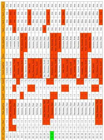
Running the trace analysis module on the basic traces generated by Diversity, we obtain 7 qualitative behaviors for the cooling system
by observing just theTcold variable. Figure 22 shows an oscillating
behavior. The red color shows when a variable changes, the green one shows the Execution context (EC) toward which the last EC in
the behavior loops back.Tcold is = Tc in EC3, then Tcold becomes
> Tc in EC7, it becomes = Tc again in EC27, it becomes < Tc in EC29, and then we loop back to EC3 where Tcold = Tc again. If
we want to see the impact of the variation ofTcold on the other
variables, we can add the first derivative ofRate as illustrated in
Figure 23. In this Figure, we see that whenTcold > Tc in EC7,
Rate is starting to increase (the first derivative of Rate is > 0 in EC9). When Tcold = Tc in EC27, Rate stops increasing ( ÛRate = 0 in EC29). When Tcold < Tc in EC29, Rate starts decreasing ( ÛRate < 0
inEC31). There is always a delay between the variation of Tcold
and ofRate because the automaton that controls the variation of
theRate is executed at the end; this automaton observes the
out-puts of our Constraint Model and then changes the variables that we want to adjust. The complete column seen in Figure 22 and Figure 23, is used to record in hyperlink the traces that included all the states variables of the system from which we have extracted the qualitative behavior shown in the behavior field. Figure 24 shows an example of a complete qualitative trace. In this figure, we see all
the state variables of the system:Heat, Thot, Tcold, Rate and also
the verification of the relations in the verification column. We see clearly that the EC toward which the last EC loops back differs from Figure 22 (EC3), Figure 23 (EC7) and Figure 24 (EC29). Although these three Figures represent the same qualitative behavior; Fig-ure 22 is refined by FigFig-ure 23 and FigFig-ure 23 is refined by FigFig-ure 24. The detection of loop back (EC) depends on the observed variables.
5
CONCLUSION
We have presented a new constraint execution model for the quali-tative simulation of cyber physical systems with only a qualiquali-tative model of the equations, with a new symbolic integration of the
Figure 20: Qualitative Relations of the Cooling system
Figure 21: Property of the operator
Figure 22: Oscillatory Behavior of Tcold
derivatives of the state variables that takes into account the cor-rective term introduced by the relations between state variables that model the continuous behavior of the system. We compute only qualitative values for the state variables by partitioning their domain into regions according to their symbolic thresholds. We compute the derivatives of the state variables by partitioning their domain into Negative, Null and Positive.
Our constraint execution model is composed of several layers of state machines. The first one contains the scenario automaton in which the user specifies the behavior of the input of the system;
Figure 23: Oscillatory Behavior of Tcold and Rate the second one contains the automata that compute the correc-tive terms of the relations that model the interactions between the different state variables of the system; the third layer contains automata that keep track of the qualitative value of the second
derivative ( Üx) of each state variable, which is symbolically
inte-grated from the previous second derivative and the corrective term linked to the second derivative; the fourth layer keeps track of the
qualitative value of the first derivative ( Ûx) of each state variable,
which is symbolically integrated from the previous first and second derivatives and the corrective terms linked to the first derivative; the fifth layer keeps track of the qualitative value of each state vari-able (x), which is symbolically integrated from the previous value, first derivative and the corrective terms linked to the value; the
Figure 24: Complete Qualitative Trace
sixth layer computes the qualitative variation of each variable by observing the automata for the qualitative value of the variable, its derivatives, and their previous value in order to detect the different qualitative variations (Constant, Increase...); the seventh layer verifies whether the relations between state variables hold or not; and finally, the eighth layer contains the automaton which models the controller specified by the user.
We have enhanced our existing tool chain, which is based on an M2M transformation from stereotyped SysML models to the HyDiv pivot language, and an M2T transformation from this lan-guage to Diversity, by designing a SysML profile for qualitative simulation without differential equations, in order to make the qual-itative modeling of cyber physical systems in SysML easier and more expressive. We have added also a filter to eliminate redundant symbolic behaviors that correspond to the same physical behavior in the execution tree generated by Diversity.
We applied our approach to a cooling system case study, which is a typical cyber physical system with logical and analog parts and is therefore a good candidate for our study. We have shown that we are able to find the different qualitative behaviors of the cooling system.
The qualitative behaviors produced by our tool chain can be used in co-simulation to validate other systems that interact with the cyber physical system. Indeed, co-simulation generally involves numerical simulators which often involve long computation time and which are necessarily configured only for specific scenarios, thus reducing the scope of exploration. In contrast, qualitative simulation provides a good abstraction of all system behaviors, which requires less computation time and thereby enables more exhaustive exploration.
There are obviously limitations to the analysis of cyber physical systems using qualitative simulation without differential equations, because behaviors that depend on specific numerical values of some parameters cannot be found. However, this approach can be applied to systems that cannot be analyzed because their differential equations are too complex to be analyzed. It can also be applied in the early phases of the design of a system, when some parameters or the exact form of the differential equations are not known yet.
REFERENCES
[1] Mathilde Arnaud, Boutheina Bannour, and Arnault Lapitre. 2016. An illustra-tive use case of the DIVERSITY Platform based on UML interaction scenarios. Electronic Notes in Theoretical Computer Science 320 (2016), 21–34.
[2] Bert Bredeweg, Floris Linnebank, Anders Bouwer, and Jochem Liem. 2009. Garp3 — Workbench for qualitative modelling and simulation. Ecological informatics 4, 5 (2009), 263–281.
[3] Christopher W. Brown. 2003. QEPCAD B: A Program for Computing with Semi-algebraic Sets Using CADs. SIGSAM Bull. 37, 4 (Dec. 2003), 97–108. https: //doi.org/10.1145/968708.968710
[4] Johan de Kleer and Daniel G Bobrow. 1984. Qualitative Reasoning With Higher-Order Derivatives.. In AAAI. 86–91.
[5] Eclipse Modeling Project. 2017. Acceleo. https://projects.eclipse.org/projects/ modeling.m2t.acceleo
[6] Eclipse Modeling Project. 2017. QVT. https://projects.eclipse.org/projects/ modeling.mmt.qvt-oml
[7] Pierre Fouché and Benjamin J Kuipers. 1992. Reasoning about energy in qual-itative simulation. IEEE Trans. on Systems, Man, and Cybernetics 22, 1 (1992), 47–63.
[8] Jean-Pierre Gallois and Agnès Lanusse. 1998. Le test structurel pour la vérifica-tion de spécificavérifica-tions de systèmes industriels: L’outil AGATHA. In Fiabilité & maintenabilité. 566–574.
[9] Jean-Pierre Gallois and Jean-Yves Pierron. 2016. Qualitative simulation and validation of complex hybrid systems. In ERTS 2016. TOULOUSE, France. https: //hal.archives-ouvertes.fr/hal-01291350
[10] Benjamin Kuipers. 1986. Qualitative simulation. Artificial intelligence 29, 3 (1986), 289–338.
[11] Benjamin Kuipers and Charles Chiu. 1987. Taming intractible branching in qualitative simulation. Readings in qualitative reasoning about physical systems (1987).
[12] Nancy Lynch, Roberto Segala, and Frits Vaandrager. 2003. Hybrid i/o automata. Information and computation 185, 1 (2003), 105–157.
[13] Slim Medimegh, Jean-Yves Pierron, and Frédéric Boulanger. 2018. Qualitative Simulation of Hybrid Systems with an Application to SysML Models. In 6th International Conference on Model-Driven Engineering and Software Development. SCITEPRESS-Science and Technology Publications.
[14] Antoine Missier and L Trave-Massuyes. 1991. Temporal information in qualitative simulation. In AI, Simulation and Planning in High Autonomy Systems. IEEE, 298– 305.
[15] Nicolas Rapin, Christophe Gaston, Arnault Lapitre, and Jean-Pierre Gallois. 2003. Behavioural unfolding of formal specifications based on communicating au-tomata. In Proc. 1st Workshop on Automated Technology for Verification and Anal-ysis.