HAL Id: hal-03208397
https://hal.archives-ouvertes.fr/hal-03208397
Submitted on 28 Apr 2021
HAL is a multi-disciplinary open access
archive for the deposit and dissemination of
sci-entific research documents, whether they are
pub-lished or not. The documents may come from
teaching and research institutions in France or
abroad, or from public or private research centers.
L’archive ouverte pluridisciplinaire HAL, est
destinée au dépôt et à la diffusion de documents
scientifiques de niveau recherche, publiés ou non,
émanant des établissements d’enseignement et de
recherche français ou étrangers, des laboratoires
publics ou privés.
C. Le Quéré, R. Andres, T. Boden, T. Conway, R. Houghton, J. House, G.
Marland, G. Peters, G. van der Werf, A. Ahlström, et al.
To cite this version:
C. Le Quéré, R. Andres, T. Boden, T. Conway, R. Houghton, et al.. The global carbon budget 1959–
2011. Earth System Science Data, Copernicus Publications, 2013, 5 (1), pp.165-185.
�10.5194/essd-5-165-2013�. �hal-03208397�
Earth Syst. Sci. Data, 5, 165–185, 2013 www.earth-syst-sci-data.net/5/165/2013/ doi:10.5194/essd-5-165-2013
©Author(s) 2013. CC Attribution 3.0 License.
History
ofGeo- and Space
Sciences
Open
Access
Advances
in Science & Research Open Access ProceedingsOpen Access Earth System
Science
Data
Open Access Earth SystemScience
Data
D iscussionsDrinking Water
Engineering and Science
Open Access
Drinking Water
Engineering and Science
Discussions O pen Acc es s
Social
Geography
Open Access D iscussionsSocial
Geography
Open AccessThe global carbon budget 1959–2011
C. Le Qu´er´e1, R. J. Andres2, T. Boden2, T. Conway3, R. A. Houghton4, J. I. House5, G. Marland6,
G. P. Peters7, G. R. van der Werf8, A. Ahlstr¨om9, R. M. Andrew7, L. Bopp10, J. G. Canadell11, P. Ciais10,
S. C. Doney12, C. Enright1, P. Friedlingstein13, C. Huntingford14, A. K. Jain15, C. Jourdain1,*, E. Kato16,
R. F. Keeling17, K. Klein Goldewijk18,19,20, S. Levis21, P. Levy14, M. Lomas22, B. Poulter10,
M. R. Raupach11, J. Schwinger23,24, S. Sitch25, B. D. Stocker26,27, N. Viovy10, S. Zaehle28, and N. Zeng29
1Tyndall Centre for Climate Change Research, University of East Anglia, Norwich Research Park,
Norwich, NR4 7TJ, UK
2Carbon Dioxide Information Analysis Center (CDIAC), Oak Ridge National Laboratory, Oak Ridge,
Tennessee, USA
3National Oceanic & Atmosphere Administration, Earth System Research Laboratory (NOAA/ESRL), Boulder,
Colorado 80305, USA
4Woods Hole Research Centre (WHRC), Falmouth, Massachusetts 02540, USA
5Cabot Institute, Dept. of Geography, University of Bristol, Bristol, UK
6Research Institute for Environment, Energy, and Economics, Appalachian State University, Boone,
North Carolina 28608, USA
7Center for International Climate and Environmental Research – Oslo (CICERO), Oslo, Norway
8Faculty of Earth and Life Sciences, VU University Amsterdam, Amsterdam, the Netherlands
9Department of Physical Geography and Ecosystem Science, Lund University, Lund, Sweden
10Laboratoire des Sciences du Climat et de l’Environnement, CEA-CNRS-UVSQ, CE Orme des Merisiers,
91191 Gif sur Yvette Cedex, France
11Global Carbon Project, CSIRO Marine and Atmospheric Research, Canberra, Australia
12Woods Hole Oceanographic Institution (WHOI), Woods Hole, Massachusetts 02543, USA
13College of Engineering, Mathematics and Physical Sciences, University of Exeter, Exeter, UK
14Centre for Ecology and Hydrology (CEH), Wallingford, OX10 8BB, UK
15Department of Atmospheric Sciences, University of Illinois, Illinois, USA
16Center for Global Environmental Research (CGER), National Institute for Environmental Studies (NIES),
Tsukuba, Japan
17University of California, San Diego, Scripps Institution of Oceanography, La Jolla, California
92093-0244, USA
18PBL Netherlands Environmental Assessment Agency, The Hague/Bilthoven, the Netherlands
19Department Innovation and Environmental Sciences (IMEW) Utrecht University, Utrecht, the Netherlands
20Institute for History and Culture (OGC), Utrecht University, Utrecht, the Netherlands
21National Center for Atmospheric Research (NCAR), Boulder, Colorado, USA
22Centre for Terrestrial Carbon Dynamics (CTCD), Sheffield University, UK
23Geophysical Institute, University of Bergen, Bergen, Norway
24Bjerknes Centre for Climate Research, Bergen, Norway
25College of Life and Environmental Sciences, University of Exeter, EX4 4RJ, Exeter, UK
26Climate and Environmental Physics, Physics Institute, University of Bern, 3012 Bern, Switzerland
27Oeschger Center for Climate Change Research, University of Bern, Bern, Switzerland
28Max-Planck-Institut f¨ur Biogeochemie, P.O. Box 600164, Hans-Kn¨oll-Str. 10, 07745 Jena, Germany
29Department of Atmospheric and Oceanic Science, University of Maryland, Maryland, USA
*now at: Food and Agriculture Organization of the United Nations (FAO), Rome, Italy
Correspondence to: C. Le Qu´er´e ([email protected])
Received: 20 November 2012 – Published in Earth Syst. Sci. Data Discuss.: 2 December 2012 Revised: 11 March 2013 – Accepted: 14 March 2013 – Published: 8 May 2013
Abstract. Accurate assessments of anthropogenic carbon
dioxide (CO2) emissions and their redistribution among the
atmosphere, ocean, and terrestrial biosphere is important to better understand the global carbon cycle, support the climate policy process, and project future climate change. Present-day analysis requires the combination of a range of data, algorithms, statistics and model estimates and their interpretation by a broad scientific community. Here we describe datasets and a methodology developed by the global carbon cycle science community to quantify all major components of the global carbon budget, including their uncertainties. We discuss changes compared to previous estimates, consistency within and among components, and
methodology and data limitations. CO2 emissions from
fossil fuel combustion and cement production (EFF) are based on energy statistics, while emissions from
Land-Use Change (ELUC), including deforestation, are based
on combined evidence from land cover change data, fire activity in regions undergoing deforestation, and models.
The global atmospheric CO2 concentration is measured
directly and its rate of growth (GATM) is computed from
the concentration. The mean ocean CO2 sink (SOCEAN) is
based on observations from the 1990s, while the annual anomalies and trends are estimated with ocean models.
Finally, the global residual terrestrial CO2 sink (SLAND) is
estimated by the difference of the other terms. For the last
decade available (2002–2011), EFF was 8.3 ± 0.4 PgC yr−1,
ELUC 1.0 ± 0.5 PgC yr−1, GATM 4.3 ± 0.1 PgC yr−1, SOCEAN
2.5 ± 0.5 PgC yr−1, and SLAND 2.6 ± 0.8 PgC yr−1. For year
2011 alone, EFF was 9.5 ± 0.5 PgC yr−1, 3.0 percent above
2010, reflecting a continued trend in these emissions; ELUC
was 0.9 ± 0.5 PgC yr−1, approximately constant throughout
the decade; GATM was 3.6 ± 0.2 PgC yr−1, SOCEAN was
2.7 ± 0.5 PgC yr−1, and S
LANDwas 4.1 ± 0.9 PgC yr−1. GATM
was low in 2011 compared to the 2002–2011 average because of a high uptake by the land probably in response to natural climate variability associated to La Ni˜na conditions
in the Pacific Ocean. The global atmospheric CO2
concentra-tion reached 391.31 ± 0.13 ppm at the end of year 2011. We
estimate that EFF will have increased by 2.6 % (1.9–3.5 %)
in 2012 based on projections of gross world product and recent changes in the carbon intensity of the economy. All uncertainties are reported as ±1 sigma (68 % confidence assuming Gaussian error distributions that the real value lies within the given interval), reflecting the current capacity to characterise the annual estimates of each component of the global carbon budget. This paper is intended to provide a baseline to keep track of annual carbon budgets in the future.
All data presented here can be downloaded from
the Carbon Dioxide Information Analysis Center
(doi:10.3334/CDIAC/GCP V2013).
1 Introduction
The concentration of carbon dioxide (CO2) in the atmo-sphere has increased from approximately 278 parts per mil-lion (ppm) in 1750, the beginning of the Industrial Era, to 391.31 at the end of 2011 (Conway and Tans, 2012). This increase was caused initially mainly by the anthropogenic release of carbon to the atmosphere from deforestation and other land-use change activities. Emissions from fossil fuel combustion started before the Industrial Era and became the dominant source of anthropogenic emissions to the atmo-sphere from around 1920 until present. Anthropogenic emis-sions occur on top of an active natural carbon cycle that cir-culates carbon between the atmosphere, ocean, and terrestrial biosphere reservoirs on timescales from days to many mil-lennia, while geologic reservoirs have even longer timescales (Archer et al., 2009).
The “global carbon budget” presented here refers to the mean, variations, and trends in the anthropogenic
perturba-tion of CO2in the atmosphere. It quantifies the input of CO2
to the atmosphere by emissions from human activities, the
growth of CO2 in the atmosphere, and the resulting changes
in land and ocean carbon fluxes directly in response to
in-creasing atmospheric CO2 levels and indirectly in response
to climate change and climate variability, and other anthro-pogenic and natural changes. An understanding of this per-turbation budget over time and the underlying variability and trends of the natural carbon cycle are necessary to understand and quantify climate-carbon feedbacks. This also allows po-tentially earlier detection of any approaching discontinuities or tipping points of the carbon cycle in response to anthro-pogenic changes (Falkowski et al., 2000).
The components of the CO2 budget that are reported in
this paper include separate estimates for (1) the CO2
emis-sions from fossil fuel combustion and cement production
(EFF); (2) the CO2emissions resulting from deliberate human
activities on land, including land use; land-use change and forestry (shortened to LUC hereafter; ELUC), (3) the growth
rate of CO2in the atmosphere (GATM); and (4) the uptake of
CO2by the “CO2sinks” in the ocean (SOCEAN) and on land
(SLAND). The CO2sinks as defined here include the response
of the land and ocean to elevated CO2 and changes in
cli-mate and other environmental conditions. The emissions and their partitioning among the atmosphere, ocean and land are in balance:
EFF+ ELUC= GATM+ SOCEAN+ SLAND. (1)
Equation (1) subsumes, and partly omits, two kinds of
pro-cesses. The first is the net input of CO2 to the atmosphere
from the chemical oxidation of reactive carbon-containing gases, primarily methane (CH4), carbon monoxide (CO), and volatile organic compounds such as terpene and isoprene, which we quantify here for the first time. The second pro-cess involves anthropogenic perturbations to carbon cycling in inland freshwaters, estuaries, and coastal areas that modify
both lateral fluxes transported from land ecosystems to the
open ocean, “vertical” CO2fluxes by outgassing in rivers and
estuaries, and the air-sea net exchange of CO2in coastal
ar-eas (Battin et al., 2008; Aufdenkampe et al., 2011). These flows are omitted in the absence of details on the natural ver-sus anthropogenic terms of these facets of the carbon cycle.
The inclusion of these fluxes of anthropogenic CO2 would
affect the estimates of SLANDand perhaps SOCEANin Eq. (1),
but not GATM.
The CO2 budget has been assessed by the
Intergovern-mental Panel on Climate Change (IPCC) in all assessment reports (Watson et al., 1990; Schimel et al., 1995; Pren-tice et al., 2001; Denman et al., 2007), and by others (Conway and Tans, 2012). These included budget estimates for the decades of the 1980s, 1990s and, most recently, the period 2000–2005. The IPCC methodology has been adapted and used by the Global Carbon Project (GCP, www. globalcarbonproject.org), who have coordinated a
coopera-tive community effort for the annual publication of global
carbon budgets up to year 2005 (Raupach et al., 2007; includ-ing fossil emissions only), year 2006 (Canadell et al., 2007),
year 2007 (published online; http://lgmacweb.env.uea.ac.uk/
lequere/co2/2007/carbon budget 2007.htm), year 2008 (Le
Qu´er´e et al., 2009), year 2009 (Friedlingstein et al., 2010), and most recently, year 2010 (Peters et al., 2012a). Each of these papers updated previous estimates with the latest avail-able information for the entire time series. From 2008, these publications projected fossil fuel emissions for one addi-tional year using the projected World Gross Domestic Prod-uct and estimated changes in the carbon intensity of the econ-omy.
We adopt a range of ±1 standard deviation (sigma) to re-port the uncertainties in our annual estimates, representing a likelihood of 68 % that the true value lies within the provided range, assuming that the errors have a Gaussian distribution.
This choice reflects the difficulty of characterising the
un-certainty in the CO2 fluxes between the atmosphere and the
ocean and land reservoirs individually, as well as the di
ffi-culty to update the CO2 emissions from LUC, particularly
on an annual basis. A 68 % likelihood provides an indication of our current capability to quantify each term and its uncer-tainty given the available information. For comparison, the Fourth Assessment Report of the IPCC (AR4) generally re-ported 90 % uncertainty for large datasets whose uncertainty
is well characterised, or for long time intervals less affected
by year-to-year variability. This includes, for instance, at-tribution statements associated with recorded warming lev-els since the pre-industrial period. The 90 % number corre-sponds to the IPCC language of “very likely” or “very high confidence represents at least a 9 out of 10 chance”; our 68 % value is near the 66 % which the IPCC reports as “likely”. The uncertainties reported here combine statistical analysis of the underlying data and expert judgement of the likelihood of results lying outside this range. The limitations of current information are discussed in the paper.
All units are presented in petagrammes of carbon (PgC,
1015gC), which is the same as gigatonnes of carbon (GtC).
Units of gigatonnes of CO2(or billion tonnes of CO2) used
in policy circles are equal to 3.67 multiplied by the value in units of PgC.
This paper provides a detailed description of the datasets and methodology used to compute the global carbon bud-get and associated uncertainties for the period 1959–2011. It presents the global carbon budget estimates by decade since the 1960s, including the last decade (2002–2011), the
results for the year 2011, and a projection of EFF for year
2012. It is intended that this paper will be updated every year using the format of “living reviews” to help keep track of new versions of the budget that result from new data, revi-sion of data, and changes in methodology. Additional ma-terials associated with the release of each new version will be posted at the Global Carbon Project (GCP) website (http: //www.globalcarbonproject.org/carbonbudget). With this ap-proach, we aim to provide transparency and traceability in reporting indicators and drivers of climate change.
2 Methods
The original data and measurements used to complete the global carbon budget are generated by multiple
organiza-tions and research groups around the world. The effort
pre-sented here is thus mainly one of synthesis, where results from individual groups are collated, analysed and evaluated for consistency. Descriptions of the measurements, models, and methodologies follow below and in depth descriptions of each component are described elsewhere (e.g. Andres et al., 2012; Houghton et al., 2012).
2.1 CO2emissions from fossil fuel combustion and
cement production (EFF)
2.1.1 Fossil fuel and cement emissions and their uncertainty
The calculation of global and national CO2 emissions from
fossil fuel combustion, including gas flaring and cement pro-duction (EFF), relies primarily on energy data, specifically data on hydrocarbon fuels, collated and archived by sev-eral organisations (Andres et al., 2012), including the Carbon Dioxide Information Analysis Center (CDIAC), the Interna-tional Energy Agency (IEA), the United Nations (UN), and the United States Department of Energy (DoE) Energy In-formation Administration (EIA). We use the emissions
esti-mated by the CDIAC (http://cdiac.ornl.gov) which are based
primarily on energy data provided by the UN Statistics Divi-sion (UN, 2012a, b; Table 1), and are typically available 2– 3 yr after the close of a given year. CDIAC also provides the only dataset that extends back in time to 1751 with consis-tent and well-documented emissions from all fossil fuels, ce-ment production, and gas flaring for all countries; this makes
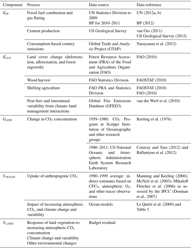
Table 1.Data sources used to compute each component of the global carbon budget.
Component Process Data source Data reference
EFF Fossil fuel combustion and
gas flaring
UN Statistics Division to 2009
UN (2012a, b)
BP for 2010–2011 BP (2012) Cement production US Geological Survey van Oss (2011)
US Geological Survey (2012) Consumption-based country
emissions
Global Trade and Analy-sis Project (GTAP)
Narayanan et al. (2012)
ELUC Land cover change
(deforesta-tion, afforestation, and forest regrowth)
Forest Resource Assess-ment (FRA) of the Food and Agriculture Organi-sation (FAO)
FAO (2010)
Wood harvest FAO Statistics Division FAOSTAT (2010) Shifting agriculture FAO FRA and Statistics
Division
FAOSTAT (2010) FAO (2010) Peat fires and interannual
variability from climate–land management interactions
Global Fire Emissions Database (GFED3)
van der Werf et al. (2010)
GATM Change in CO2concentration 1959–1980: CO2
Pro-gram at Scripps Insti-tution of Oceanography and other research groups
Keeling et al. (1976)
1980–2011: US National Oceanic and Atmo-spheric Administration Earth System Research Laboratory
Conway and Tans (2012) and Ballantyne et al. (2012)
SOCEAN Uptake of anthropogenic CO2 1990–1999 average:
in-direct estimates based on CFCs, atmospheric O2,
and other tracer observa-tions
Manning and Keeling (2006); McNeil et al. (2003); Mikaloff Fletcher et al. (2006) as as-sessed by the IPCC (Denman et al., 2007)
Impact of increasing atmospheric CO2, and climate change and
variability
Ocean models Le Qu´er´e et al. (2009) and Table 3
SLAND Response of land vegetation to:
increasing atmospheric CO2
concentration
Budget residual
Climate change and variability Other environmental changes
the dataset a unique resource for research of the carbon cy-cle during the fossil fuel era. For this paper, we use CDIAC emissions data from the period 1959–2009, and preliminary estimates based on the BP annual energy review for extrap-olation of emissions in 2010 and 2011 (BP, 2012). BP’s sources for energy statistics overlap with those of the UN data but are compiled more rapidly, using a smaller group
of mostly developed countries and assumptions for missing data. We use the BP values only for the year-to-year rate of change, because the rates of change are less uncertain than the absolute values. The preliminary estimates are re-placed by the more complete CDIAC data when available. Past experience shows that projections based on the BP rate of change provide reliable estimates for the two most recent
years when full data are not yet available from the UN (see Sect. 3.2).
Emissions from cement production are based on cement data from the US Geological Survey (van Oss, 2011) up to year 2009, and from preliminary data for 2010 and 2011 (US Geological Survey, 2012). Emission estimates from gas flar-ing are calculated in a similar manner as those from solid, liquid, and gaseous fuels, and rely on the UN Energy Statis-tics to supply the amount of flared fuel. For emission years 2010 and 2011, flaring estimates are assumed constant from the emission year 2009 UN-based data. The basic data on gas flaring have large uncertainty. Fugitive emissions of CH4 from the so-called upstream sector (coal mining, oil extrac-tion, gas extraction and distribution) are not included in the
accounts of CO2emissions except to the extent that they get
captured in the UN energy data and counted as gas “flared or lost”. The UN data are not able to distinguish between gas that is flared or vented.
When necessary, fuel masses/volumes are converted to
fuel energy content using coefficients provided by the UN
and then to CO2emissions using conversion factors that take
into account the relationship between carbon content and
heat content of the different fuel types (coal, oil, gas, gas
flaring) and the combustion efficiency (to account, for
ex-ample, for soot left in the combustor or fuel otherwise lost
or discharged without oxidation). In general, CO2emissions
for equivalent energy consumptions are about 30 % higher for coal compared to oil, and 70 % higher for coal compared to gas (Marland et al., 2007). These calculations are based on the mass flows of carbon and assume that the carbon
dis-charged, such as CO or CH4, will soon be oxidized to CO2in
the atmosphere and hence counts the carbon mass with CO2
emissions.
Emissions are estimated for 1959–2011 for 129 countries and regions. The disaggregation of regions (e.g. the former Soviet Union prior to 1992) is based on the shares of emis-sions in the first year after the countries were disaggregated.
Estimates of CO2 emissions show that the global total of
emissions is not equal to the sum of emissions from all coun-tries. This is largely attributable to combustion of fuels used in international shipping and aviation, where the emissions are included in the global totals but are not attributed to indi-vidual countries. In practice, the emissions from international bunker fuels are calculated based on where the fuels were loaded, but they are not included with national emissions
es-timates. Smaller differences also occur because globally, the
sum of imports in all countries is not equivalent to the sum
of exports, due to differing treatment of oxidation of non-fuel
uses of hydrocarbons (e.g. as solvents, lubricants, feedstocks, etc.).
The uncertainty of the annual fossil fuel and cement emis-sions for the globe has been estimated at ±5 % (scaled down from the published ±10 % at ±2 sigma to the use of ±1 sigma bounds reported here; Andres et al., 2012). This includes an assessment of the amounts of fuel consumed, the carbon
con-tents of fuels, and the combustion efficiency. While in the
budget we consider a fixed uncertainty of ±5 % for all years, in reality the uncertainty, as a percentage of the emissions, is growing with time because of the larger share of global emissions from non-Annex B countries with weaker statis-tical systems (Marland et al., 2009). For example, the un-certainty in Chinese emissions estimates has been estimated at around ±10 % (±1 sigma; Gregg et al., 2008). Generally, emissions from mature economies with good statistical bases have an uncertainty of only a few percent (Marland, 2008). Further research is needed before we can quantify the time evolution of the uncertainty.
2.1.2 Emissions embodied in goods and services
National emissions inventories take a territorial (production) perspective by “include[ing] all greenhouse gas emissions and removals taking place within national (including
admin-istered) territories and offshore areas over which the country
has jurisdiction” (from the Revised 1996 IPCC Guidelines for National Greenhouse Gas Inventories). That is, sions are allocated to the country where and when the emis-sions actually occur. The emission inventory of an individ-ual country does not include the emissions from the produc-tion of goods and services produced in other countries (e.g. food and clothes) that are used for national consumption. The
difference between the standard territorial emission
invento-ries and consumption-based emission inventoinvento-ries is the net transfer (exports minus imports) of emissions from the pro-duction of internationally traded goods and services. Com-plementary emission inventories that allocated emissions to the final consumption of goods and services (e.g. Davis and Caldeira, 2010) provide additional information that can be used to understand emission drivers, quantify emission
leak-ages between countries, and potentially design more effective
and efficient climate policy.
We estimate consumption-based emissions by enumerat-ing the global supply chain usenumerat-ing a global model of the eco-nomic relationships between sectors in every country (Pe-ters et al., 2011a). Due to availability of the input data, de-tailed estimates are made for the years 1997, 2001, 2004, and 2007 (an extension of Peters et al., 2011b) using economic and trade data from the Global Trade and Analysis Project (GTAP; Narayanan et al., 2012). The results cover 57 sec-tors and up to 129 countries and regions. The results are ex-tended into an annual time series from 1990 to the latest year of the fossil-fuel emissions or GDP data (2010 in this bud-get), using GDP data by expenditure (from the UN Main Ag-gregates database; UN, 2012c) and time series of trade data from GTAP (Narayanan et al., 2012). We do not provide an uncertainty estimate for these emissions, but based on model comparisons and sensitivity analysis, they are unlikely to be significantly larger than for the territorial emission estimates (Peters et al., 2012b). Uncertainty is expected to increase for more detailed results (Peters et al., 2011b; e.g. the results for
Annex B will be more accurate than the sector results for an individual country).
It is important to note that the consumption-based emis-sions defined here consider directly the carbon embodied in traded goods and services, but not the trade in unoxidised fossil fuels (coal, oil, gas). In our consumption-based inven-tory, emissions from traded fossil fuels accrue to the coun-try where the fuel is burned or consumed, not the exporting country from which it was extracted (Davis et al., 2011).
The consumption-based emission inventories in this car-bon budget have several improvements over previous ver-sions (Peters et al., 2011b, 2012a). The detailed estimates for 2004 and 2007 are based on an updated version of the GTAP database (Narayanan et al., 2012). We estimate the sector
level CO2emissions using our own calculations based on the
GTAP data and methodology, but scale the national totals to match the CDIAC estimates from the carbon budget. We do not include international transportation in our estimates. The time series of trade data provided by GTAP covers the pe-riod 1995–2009 and our methodology uses the trade shares of this dataset. For the period 1990–1994 we assume the trade shares of 1995, while in 2010 we assume the trade shares of
2008, since 2009 was heavily affected by the global financial
crisis. We identified errors in the trade shares of Taiwan and the Netherlands in 2008 and 2009, and for these two coun-tries, the trade shares for 2008–2010 are based on the 2007 trade shares.
These data do not contribute to the global average terms in Eq. (1), but are relevant to the anthropogenic carbon cy-cle, as they reflect the movement of carbon across the Earth’s surface in response to human needs (both physical and eco-nomic). Furthermore, if national and international climate policies continue to develop in an unharmonious way, then the trends reflected in these data will need to be accommo-dated by those developing policies.
2.1.3 Emissions projections for the current year
Energy statistics are normally available around June for the previous year. We use the close relationship between the growth in world Gross Domestic Product (GDP) and the growth in global emissions (Raupach et al., 2007) to project emissions for the current year. This is based on the so-called
Kaya (also called IPAT) identity, whereby EFFis decomposed
by the product of GDP and the fossil fuel carbon intensity of
the economy (IFF) as follows:
EFF= GDP · IFF; (2)
taking a time derivative of this equation gives: dEFF
dt =
d(GDP · IFF)
dt ; (3)
and applying the rules of calculus, assuming that GDP and
IFFare independent: dEFF dt = dGDP dt · IFF+ GDP · dIFF dt ; (4)
finally, dividing Eqs. (4) by (2) gives: 1 EFF dEFF dt = 1 GDP dGDP dt + 1 IFF dIFF dt , (5)
where the left hand term is the relative growth rate of EFF, and the right hand terms are the relative growth rates of GDP
and IFF, respectively, which can simply be added linearly to
give overall growth rate. The growth rates are reported in per-cent below by multiplying each term by 100. Because pre-liminary estimates of annual change in GDP are made well before the end of a calendar year, making assumptions on the
growth rate of IFFallows us to make projections of the annual
change in CO2 emissions well before the end of a calendar
year.
2.1.4 Growth rate in emissions
We report the annual growth rate in emissions for adjacent
years in percent by calculating the difference between the
two years and then comparing to the emissions in the first
year: [(EFF(t0+ 1) − EFF(t0))/EFF(t0)] · 100. This is the
sim-plest method to characterise a one-year growth compared to the previous year. This has strong links with the more general way in which society presents economic change in journalis-tic circles, most often a comparison of present-day economic activity compared to the previous year.
The growth rate of EFFover time periods of greater than
one year can be re-written using its logarithm equivalent as follows: 1 EFF dEFF dt = d(ln EFF) dt . (6)
Here we calculate growth rates in emissions for multi-year periods (e.g. a decade) by fitting a linear trend to ln (EFF) in Eq. (6), reported in percent per year. We fit the logarithm of
EFFrather than EFFdirectly because this method ensures that
computed growth rates satisfy Eq. (5). This method differs
from previous papers (Canadell et al., 2007; Le Qu´er´e et al.,
2009), who computed the fit to EFFand divided by average
EFFdirectly, but the difference is very small (< 0.05 percent)
in the case of EFF.
2.2 CO2emissions from land use, land-use change and
forestry (ELUC)
Net LUC emissions reported in our annual budget (ELUC)
in-clude CO2 fluxes from afforestation, deforestation, logging
(forest degradation and harvest activity), shifting cultivation (cycle of cutting forest for agriculture then abandoning), re-growth of forests following wood harvest or abandonment of agriculture, fire-based peatland emissions and other land management practices (Table 2). Our annual estimate com-bines information from a bookkeeping model (Sect. 2.2.1) primarily based on forest area change and biomass data from
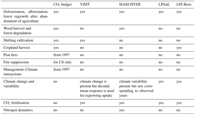
Table 2.Comparison of the processes included in the ELUCof the global carbon budget and the DGVMs. See Table 3 for model references.
CO2budget VISIT ISAM-HYDE LPJmL LPJ-Bern
Deforestation, afforestation, forest regrowth after aban-donment of agriculture
yes yes yes yes yes
Wood harvest and forest degradation
yes no yes no no
Shifting cultivation yes yes no no no Cropland harvest yes no no no yes Peat fires from 1997 no no no no Fire suppression for US only no no no no Management–Climate
interactions
from 1997 no no no no
Climate change and variability
no climate change is present but decadal mean response is used for regrowing uptake
climate variability present but not corre-sponding to observed years
yes yes
CO2fertilisation no yes yes yes yes
Nitrogen dynamics no no yes no no
the Forest Resource Assessment (FRA) of the Food and Agri-culture Organisation (FAO; Houghton, 2003) published at in-tervals of five years, with annual emissions estimated from satellite-based fire activity in deforested areas (Sect. 2.2.2; van der Werf et al., 2010). The bookkeeping model is used
mainly to quantify the mean ELUC over the time period of
the available data, and the satellite-based method to dis-tribute these emissions annually. The satellite-based emis-sions are available from year 1997 onwards only. We cal-culate the global anomaly in satellite-based emissions over deforested regions, compared to the 1997–2011 time period,
and add this to average ELUCestimated using the
bookkeep-ing method. We thus assume that all land management ac-tivities apart from deforestation do not vary significantly on a year-to-year basis. Other sources of interannual variabil-ity (e.g. the impact of climate variabilvariabil-ity on regrowth) are
accounted for in SLAND. We also use independent estimates
from Dynamic Global Vegetation Models (Sect. 2.2.3) to help quantify the uncertainty in global ELUC.
2.2.1 Bookkeeping method
ELUC calculated using a bookkeeping method (Houghton,
2003) keeps track of the carbon stored in vegetation and soils before deforestation or other land-use change, and the changes in forest age classes, or cohorts, of disturbed lands
after land-use change. It tracks the CO2emitted to the
atmo-sphere over time due to decay of soil and vegetation carbon
in different pools, including wood products, pools after
log-ging and deforestation. It also tracks the regrowth of vege-tation and build-up of soil carbon pools following land-use change. It considers transitions between forests, pastures and cropland, shifting cultivation, degradation of forests where a fraction of the trees is removed, abandonment of agricultural land, and forest management such as logging and fire man-agement. In addition to tracking logging debris on the forest floor, the bookkeeping model tracks the fate of carbon con-tained in harvested wood products that is eventually emitted
back to the atmosphere as CO2, although a detailed treatment
of the lifetime in each product pool is not performed (Earles et al., 2012). Harvested wood products are partitioned into
three pools with different turnover times. All fuelwood is
as-sumed to be burned in the year of harvest (1.0 yr−1). Pulp
and paper products are oxidized at a rate of 0.1 yr−1. Timber
is assumed to be oxidized at a rate of 0.01 yr−1, and elemental
carbon decays at 0.001 yr−1. The general assumptions about
partitioning wood products among these pools are based on national harvest data.
The primary land cover change and biomass data for the bookkeeping model analysis is the FAO FRA 2010 (FAO, 2010; Table 1), which is based on countries’ self-reporting of statistics on forest cover change and management par-tially combined with satellite data in more recent assess-ments. Changes in land cover other than forest are based on annual, national changes in cropland and pasture areas re-ported by the FAO Statistics Division (FAOSTAT, 2010). The LUC dataset is non-spatial and aggregated by regions. The carbon stocks on land (biomass and soils), and their response
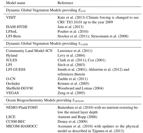
Table 3.References for the process models included in Fig. 3. Model name Reference Dynamic Global Vegetation Models providing ELUC
VISIT Kato et al. (2013) Climate forcing is changed to use CRU TS3.10.01 up to the year 2009
ISAM-HYDE Jain et al. (2013) LPJmL Poulter et al. (2010)
LPJ-Bern Stocker et al. (2011); Strassmann et al. (2008) Dynamic Global Vegetation Models providing SLAND
Community Land Model 4CN Lawrence et al. (2011) Hyland Levy et al. (2004)
JULES Clark et al. (2011); Cox (2001) LPJ Sitch et al. (2003)
LPJ-GUESS Smith et al. (2001); Ahlstr¨om et al. (2012) and references therein
O-CN Zaehle et al. (2011) Orchidee Krinner et al. (2005) Sheffield-DGVM Woodward and Lomas (2004) VEGAS Zeng et al. (2005)
Ocean Biogeochemistry Models providing SOCEAN
NEMO-PlankTOM5 Buitenhuis et al. (2010) with no nutrient restoring be-low the mixed layer depth
LSCE Aumont and Bopp (2006) CCSM-BEC Doney et al. (2009)
MICOM-HAMOCC Assmann et al. (2010) with updates to the physical model as described in Tjiputra et al. (2013)
functions subsequent to LUC, are based on averages per land cover type, per biome and per region. Similar results were obtained using forest biomass carbon density based on satel-lite data (Baccini et al., 2012). The bookkeeping model does not include land ecosystems’ transient response to changes in
climate, atmospheric CO2 and other environmental factors,
but the growth/decay curves are based on contemporary data
that will implicitly reflect the effects of CO2and climate at
that time. Results from the bookkeeping method are available from 1850 to 2010.
2.2.2 Fire-based method
LUC CO2 emissions calculated from satellite-based fire
ac-tivity in deforested areas (van der Werf et al., 2010) provide information that is complementary to the bookkeeping ap-proach. Although they do not provide a direct estimate of
ELUC, as they do not include processes such as respiration,
wood harvest, wood products or forest regrowth, they do
provide insight on the year-to-year variations in ELUC that
result from the interactions between climate and human ac-tivity (e.g. there is more burning and clearing of forests in dry years). The “deforestation fire emissions” assumes an im-portant role of fire in removing biomass in the deforestation
process, and thus can be used to infer direct CO2emissions
from deforestation using satellite-derived data on fire activity in regions with active deforestation (legacy emissions such as decomposition from ground debris or soils are missed by this method). The method requires information on the frac-tion of total area burned associated with deforestafrac-tion versus other types of fires, and can be merged with information on biomass stocks and the fraction of the biomass lost in a
defor-estation fire to estimate CO2 emissions. The satellite-based
fire emissions are limited to the tropics, where fires result mainly from human activities. Tropical deforestation is the largest and most variable single contributor to ELUC.
Here we used annual estimates from the Global Fire
Emissions Database (GFED3), available from http://www.
globalfiredata.org. Burned area from (Giglio et al., 2010) is merged with active fire retrievals to mimic more sophisti-cated assessments of deforestation rates in the pan-tropics (van der Werf et al., 2010). This information is used as in-put data in a modified version of the satellite-driven CASA biogeochemical model to estimate carbon emissions, keeping track of what fraction was due to deforestation (van der Werf
et al., 2010). The CASA model uses different assumptions
to compute delay functions compared to the bookkeeping model, and does not include historical emissions or regrowth from land-use change prior to the availability of satellite data.
Comparing coincident CO emissions and their atmospheric fate with satellite-derived CO concentrations allows for some validation of this approach (e.g. van der Werf et al., 2008). In this paper, we only use emissions based on deforestation fires
to quantify the interannual variability in ELUC. Results from
the fire-based method are available from 1997 to 2011.
2.2.3 Dynamic Global Vegetation Models (DGVMs) and uncertainty assessment for LUC
Net LUC CO2 emissions have also been estimated using
DGVMs that explicitly represent some processes of vege-tation growth, mortality and decomposition associated with natural cycles and also provide a response to prescribed land
cover change and climate and CO2 drivers (Table 2). The
DGVMs calculate the dynamic evolution of biomass and soil
carbon pools that are affected by environmental variability
and change in addition to LUC transitions each year. They are independent from the other budget terms except for their
use of atmospheric CO2concentration to calculate the
fertil-ization effect of CO2 on primary production. The DGVMs
do not exactly provide ELUCas defined in this paper because
they represent fewer processes resulting directly from hu-man activities on land, but include the vegetation and soil
response to increasing atmospheric CO2 levels, to climate
variability and change (in three models), in addition to atmo-spheric N deposition in the presence of nitrogen limitation (in one model; Table 2). Nevertheless all methods represent
deforestation, afforestation and regrowth, three of the most
important components of ELUC, and thus the model spread
can help quantify the uncertainty in ELUC.
The DGVMs used here prescribe land cover change from the HYDE spatially gridded datasets updated to 2009 (Gold-ewijk et al., 2011; Hurtt et al., 2011), which is based on FAO statistics of change in agricultural areas (FAOSTAT, 2010) with assumptions made about change in forest or other land cover as a result of agricultural area change. The changes in agricultural areas are then implemented within each model (for instance, an increased cropland fraction in a grid cell can either use pasture land, or forest, the
lat-ter resulting into deforestation). This differs with the dataset
used in the bookkeeping method (Houghton, 2003 and up-dates), which is based on forest area change statistics (FAO,
2010). The DGVMs also represent a different methodology
of calculating carbon fluxes, and thus provide an indepen-dent assessment of LUC emissions to the bookkeeping re-sults (Sect. 2.2.1).
Differences between estimates thus originate from three
main sources, firstly the land cover change dataset, secondly
different approaches in models, and thirdly different process
boundaries (Table 2). Four different DGVM estimates are
presented here and used to explore the uncertainty in LUC annual emissions (Jain et al., 2013; Kato et al., 2013; Poul-ter et al., 2010; Stocker et al., 2011). While many published DGVM LUC emissions estimates exist, these model runs
were driven by a consistently updated HYDE LUC dataset up to year 2009.
We examine the standard deviation of the annual
esti-mates to assess the uncertainty in ELUC. The standard
de-viation across models in each year ranged from 0.09 to
0.70 PgC yr−1, with an average of 0.42 PgC yr−1from 1960
to 2009. One of the four models (Jain et al., 2013) was
used with three different LUC datasets (including HYDE
and FAO FRA2005; Jain et al., 2013; Meiyappan and Jain, 2012). The standard deviation for decadal means in these
three model runs was ±0.19 PgC yr−1 for 1990 to 2005, and
ranged from 0.06 to 0.70 PgC yr−1for annual estimates with
an average of ±0.27 PgC yr−1from 1960 to 2005. Assuming
the two sources of uncertainty are independent, we can com-bine them using standard error propagation rules. Taking the quadratic sum of the mean annual standard deviation across
the four DGVMs (0.42 PgC yr−1) and the standard deviation
due to different land cover change datasets (0.27 PgC yr−1)
we get a combined standard deviation of 0.5 PgC yr−1.
We use the combined standard deviation ±0.5 PgC yr−1as
a quantitative measure of uncertainty for annual emissions, and to reflect our best value judgment that there is at least 68 % chance (±1 sigma) that the true LUC emis-sion lies within the given range, for the range of processes considered here. However, we note that missing processes such as the decomposition of drained tropical peatlands (Ballhorn et al., 2009; Hooijer et al., 2010) could introduce biases which are not quantified here, while the inclusion of the impact of climate variability on land processes by some DGVMs (Table 2) may inflate the standard deviation in an-nual estimates of LUC emissions compared to our definition
of ELUC. The uncertainty of ±0.5 PgC yr−1is slightly lower
than that of ±0.7 PgC yr−1 estimated in the 2010 CO
2
bud-get release (Friedlingstein et al., 2010) based on expert as-sessment of the available estimates. A more recent expert assessment of uncertainty for the decadal mean based on a larger set of published model and uncertainty studies
esti-mated ±0.5 PgC yr−1(Houghton et al., 2012) which partly
re-flects improvements in data on forest area change using satel-lite data, and partly more complete understanding and
rep-resentation of processes in models. We adopt ±0.5 PgC yr−1
here for the decadal averages presented Table 4.
The errors in the decadal mean estimates from the DGVM ensemble are likely correlated between decades. They come from (1) system boundaries (e.g. not counting forest degrada-tion in some models), which cause a bias that makes decadal estimates perfectly correlated (Gasser and Ciais, 2013; Ta-ble 2); (2) common land cover change input data which cause
a bias, though if a different input dataset is used each decade,
decadal fluxes from DGVMs may be partly decorrelated; (3) model structural errors, which cause bias that correlate decadal estimates. In addition, errors arising from uncertain DGVM parameter values would be random but they are not accounted for in this study, since no DGVM provided an en-semble of runs with perturbed parameters.
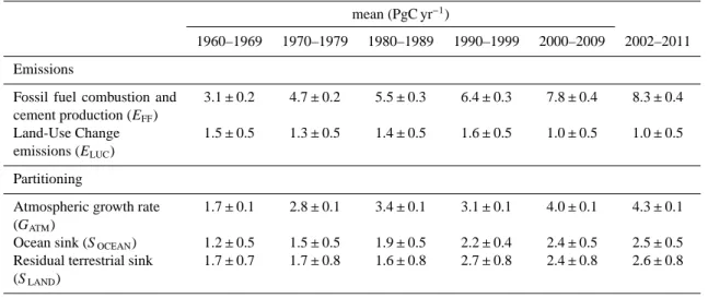
Table 4.Decadal mean in the five components of the anthropogenic CO2budget for the periods 1960–1969, 1970–1979, 1980–1989, 1990–
1999, 2000–2009 and the last decade available. All values are in PgC yr−1. All uncertainties are reported as ±1 sigma (68 % confidence
assuming Gaussian error distributions that the real value lies within the given interval).
mean (PgC yr−1)
1960–1969 1970–1979 1980–1989 1990–1999 2000–2009 2002–2011 Emissions
Fossil fuel combustion and cement production (EFF) 3.1 ± 0.2 4.7 ± 0.2 5.5 ± 0.3 6.4 ± 0.3 7.8 ± 0.4 8.3 ± 0.4 Land-Use Change emissions (ELUC) 1.5 ± 0.5 1.3 ± 0.5 1.4 ± 0.5 1.6 ± 0.5 1.0 ± 0.5 1.0 ± 0.5 Partitioning
Atmospheric growth rate (GATM)
1.7 ± 0.1 2.8 ± 0.1 3.4 ± 0.1 3.1 ± 0.1 4.0 ± 0.1 4.3 ± 0.1
Ocean sink (SOCEAN) 1.2 ± 0.5 1.5 ± 0.5 1.9 ± 0.5 2.2 ± 0.4 2.4 ± 0.5 2.5 ± 0.5
Residual terrestrial sink (SLAND)
1.7 ± 0.7 1.7 ± 0.8 1.6 ± 0.8 2.7 ± 0.8 2.4 ± 0.8 2.6 ± 0.8
2.3 Atmospheric CO2growth rate (GATM)
2.3.1 Global atmospheric CO2growth rate estimates
The atmospheric CO2growth rate is provided by the US
Na-tional Oceanic and Atmospheric Administration Earth Sys-tem Research Laboratory (Conway and Tans, 2012), which is updated from Ballantyne et al. (2012). For the 1959–1980 period, the global growth rate is based on measurements of
atmospheric CO2 concentration averaged from the Mauna
Loa and South Pole stations, as observed by the CO2
Pro-gram at Scripps Institution of Oceanography (Keeling et al., 1976). For the 1980–2011 time period, the global growth rate is based on the average of multiple stations selected from the marine boundary layer sites (Ballantyne et al., 2012), after fitting each station with a smoothed curve as a func-tion of time, and averaging by latitude band (Masarie and Tans, 1995). The annual growth rate is estimated from
at-mospheric CO2 concentration by taking the average of the
most recent and December–January months corrected for the average seasonal cycle and subtracting this same average one
year earlier. The growth rate in units of ppm yr−1is converted
to fluxes by multiplying by a factor of 2.123 PgC per ppm (Enting et al., 1994) for comparison with the other compo-nents.
The uncertainty around the annual growth rate based on the multiple stations dataset ranges between 0.11 and
0.72 PgC yr−1, with a mean of 0.61 PgC yr−1for 1959–1980
and 0.18 PgC yr−1for 1980–2011, when a larger set of
sta-tions were available. It is based on the number of avail-able stations, and thus takes into account both the measure-ment errors and data gaps at each station. This uncertainty
is larger than the uncertainty of ±0.1 PgC yr−1 reported for
decadal mean growth rate by the IPCC because errors in an-nual growth rate are strongly anti-correlated in consecutive
years leading to smaller errors for longer timescales. The
decadal change is computed from the difference in
concentra-tion ten years apart based on measurement error of 0.35 ppm
(based on offsets between NOAA/ESRL measurements and
those of the World Meterological Organisation World Data
Center for Greenhouse Gases; NOAA/ESRL, 2012) for the
start and end points (the decadal change uncertainty is the
sqrt(2 × (0.35 ppm)2)/10 yr assuming that each yearly
mea-surement error is independent). This uncertainty is also used in Table 4.
2.3.2 Assessing the contribution of anthropogenic CO and CH4to the global anthropogenic CO2budget
Emissions of CO and CH4 to the atmosphere are assumed
to be mainly balanced by natural land CO2sinks for all
bio-genic carbon compounds, but small imbalances arise through
anthropogenic emissions of fugitive fossil fuel CH4and CO,
and changes in oxidation rates, e.g. in response to climate variability. These contributions are omitted in Eq. (1), but quantified in this section to highlight the current understand-ing about their magnitude, and identify the sources of un-certainty. Emissions of CO from combustion processes are
included with EFF and ELUC (for example, CO emissions
from fires associated with LUC are included in ELUC).
How-ever, fugitive anthropogenic emissions of fossil CH4(e.g. gas
leaks) from the coal, oil and gas upstream sectors are not
counted in EFFbecause these leaks are not inventoried in the
fossil fuel statistics as they are not consumed as fuel. In the absence of anthropogenic change, natural sources
of CO and CH4 from wildfires and CH4 wetlands are
as-sumed to be balanced by CO2uptake by photosynthesis on
continental and long timescales (e.g. decadal or longer). An-thropogenic land-use change (e.g. biomass burning for forest
clearing or land management, wetland management) and the
indirect anthropogenic effects of climate change on wildfires
and wetlands result in an imbalance of sources and sinks of carbon. For the purposes of this study, we assume wildfire
and wetland emissions of CO and CH4 are in balance, and
that the non-industrial anthropogenic biogenic sources are
captured within estimates of emissions of CO2 from LUC
(included in Sect. 2.2). Peatland draining results in a
reduc-tion of CH4 emissions and an increase in CO2(not included
in modelled estimates presented here). Thus, none of the CO
and CH4 sources above are included in the (anthropogenic)
CO2budget of this study.
By contrast to biogenic sources, CO and CH4 emissions
from fossil fuel use are not balanced by any recent CO2
up-take by photosynthesis, and hence represent a net addition of fossil carbon to the atmosphere. This is implicitly included in
this study as estimates of CO2emissions are based on the
to-tal carbon content of the fuel, and the measured CO2growth
rate includes CO2from CO.
This is not the case for anthropogenic fossil CH4
emis-sion from fugitive emisemis-sions during natural gas extraction and transport, and from the coal and oil industry (gas leaks). This emission of carbon to the atmosphere is not included
in the fossil fuel CO2emissions described in Sect. 2.1. This
CH4emission is estimated at 0.09 Pg C yr−1(Kirschke et al.,
2013). Fossil CH4emissions are assumed to be oxidized with
a lifetime of 12.4 yr, the e-folding time of an atmospheric per-turbation removal (Prater et al., 2012). After one year, 92 %
of these emissions remain in the atmosphere as CH4and
con-tribute to the observed CH4 global growth rate, whereas the
rest (8 %) get oxidized into CO2, and contribute to the CO2
growth rate. Given that anthropogenic fossil fuel CH4
emis-sions represent a fraction of 15 % of the total global CH4
source (Kirschke et al., 2013), we assumed that a fraction of 0.15 times 0.92 of the observed global growth rate of CH4
of 6 Tg C-CH4yr−1 (units of C in CH4 form) during 2000–
2009 is due to fossil CH4 sources. Therefore, annual
fos-sil fuel CH4 emissions contribute 0.8 Tg C-CH4yr−1 to the
CH4 growth rate and 0.8 Tg C-CO2yr−1 (units of C in CO2
form) to the CO2growth rate. Summing up the effect of
fos-sil fuel CH4 emissions from each previous year during the
past 10 yr, a fraction of which is oxidized into CO2 in the
current year, this defines a contribution of 5 Tg C-CO2yr−1
to the CO2 growth rate, or about 0.1 %. Thus the effect of
anthropogenic fossil CH4fugitive emissions and their
oxida-tion to anthropogenic CO2in the atmosphere can be assessed
to have a negligible effect on the observed CO2growth rate,
although they do contribute significantly to the global CH4
growth rate.
2.4 Ocean CO2sink
A mean ocean CO2sink of 2.2 ± 0.4 PgC yr−1for the 1990s
was estimated by the IPCC (Denman et al., 2007) based on
three data-based methods (Mikaloff Fletcher et al., 2006;
Ta-ble 1). Here we adopt this mean CO2 sink (Manning and
Keeling, 2006; McNeil et al., 2003), and compute the trends
in the ocean CO2 sink for 1959–2011 using a combination
of five global ocean biogeochemistry models (Table 3). The models represent the physical, chemical and biological pro-cesses that influence the surface ocean concentration of CO2
and thus the air-sea CO2flux. The models are forced by
me-teorological reanalysis data and atmospheric CO2
concentra-tion available for the entire time period. They compute the
air-sea flux of CO2 over grid boxes of 1 to 4 degrees in
lat-itude and longlat-itude. The ocean CO2 sink for each model is
normalised to the observations, by dividing the annual model values by their observed average over 1990–1999, and
mul-tiplying this by 2.2 PgC yr−1. This normalisation ensures that
the ocean CO2sink for the global carbon budget is based on
observations, and that the trends and annual values in CO2
sinks are consistent with model estimates. The ocean CO2
sink for each year (t) is therefore:
SOCEAN(t)=1 n X m Sm OCEAN(t) Sm OCEAN(1990–1999) · 2.2 PgC yr−1, (7)
where n is the number of models. We use the four models published in Le Qu´er´e et al. (2009), including updates of Aumont and Bopp (2006), Doney et al. (2009), and Buiten-huis et al. (2010) available to 2011, the model results from Galbraith et al. (2010) available to 2008, and one further model estimate updated from Assman et al. (2010) also
avail-able to 2011. The mean ocean CO2 sink from these
mod-els for 1990–1999 ranges between 1.55 and 2.59 PgC yr−1.
The standard deviation of the ocean model ensemble
aver-ages to 0.14 PgC yr−1 during 1980–2011 (with a maximum
of 0.22), but it increases as the model ensemble goes back in
time, with a standard deviation of 0.3 PgC yr−1across
mod-els in the 1960s and 0.49 PgC yr−1in year 1959. We estimate
that the uncertainty in the annual ocean CO2 sink is about
±0.5 PgC yr−1from the quadratic sum of the data uncertainty
of ±0.4 PgC yr−1and standard deviation across model of up
to ±0.3 PgC yr−1, reflecting both the uncertainty in the mean
sink and in the interannual variability as assessed by models.
2.5 Terrestrial CO2sink
The difference between the fossil fuel (EFF) and LUC net
emissions (ELUC), the atmospheric growth rate (GATM) and
the ocean CO2 sink (SOCEAN) is attributable to the net sink
of CO2in terrestrial vegetation and soils (SLAND), within the
given uncertainties. Thus, this sink can be estimated either as the residual of the other terms in the mass balance budget
but also directly calculated using DGVMs. Note the SLAND
term does not include gross land sinks directly resulting from LUC (e.g. regrowth of vegetation) as these are estimated as part of the net land use flux (ELUC). The residual land sink
(SLAND) is in part due to the fertilising effect of rising
change effects such as prolonged growing seasons in north-ern temperate areas.
2.5.1 Residual of the budget
For 1959–2011, the terrestrial carbon sink was estimated from the residual of the other budget terms:
SLAND= EFF+ ELUC− (GATM+ SOCEAN). (8)
The uncertainty in SLAND is estimated annually from the
quadratic sum of the uncertainty in the right-hand terms as-suming the errors are not correlated. The uncertainty
aver-ages to ±0.8 PgC yr−1over 1959–2011, increasing with time
to ±0.93 PgC yr−1in 2011. S
LANDestimated from the
resid-ual of the budget will include, by definition, all the miss-ing processes and potential biases in the other components of Eq. (8).
2.5.2 DGVMs
A comparison of the residual calculation of SLANDin Eq. (8)
with outputs from DGVMs similar to those described in
Sect. 2.2.3, but designed to quantify SLAND rather than
ELUC, provides an independent estimate of the consistency
of SLAND with our understanding of the functioning of the
terrestrial vegetation in response to CO2 and climate
vari-ability. An ensemble of nine DGVMs are presented here, co-ordinated by the project “trends and drivers of the regional-scale sources and sinks of carbon dioxide (Trendy)” (Table 3). These DGVMs were forced with changing climate and
atmospheric CO2 concentration, and a fixed contemporary
cropland distribution. These models thus include all climate
variability and CO2effects over land, but do not include the
trend in CO2 sink capacity associated with human activity
directly affecting changes in vegetation cover and
manage-ment. This effect has been estimated to have lead to a
reduc-tion in the terrestrial sink by 0.5 PgC yr−1 since 1750 (Gitz
and Ciais, 2003) but it is neglected here. The models estimate
the mean and variability of SLANDbased on atmospheric CO2
and climate, and thus both terms can be compared to the bud-get residual.
The standard deviation of the annual CO2 sink across the
nine DGVMs ranges from ±0.2 to ±1.3 PgC yr−1, with an
average of ±0.7 PgC yr−1 for the period 1960 to 2009. This
is an improvement from the 0.95 PgC yr−1 presented in Le
Qu´er´e et al. (2009) using an ensemble of five models. As this standard deviation across the DGVM models and around the mean trends is of the same magnitude as the combined uncertainty due to the other components (EFF, ELUC, GATM,
SOCEAN), the DGVMs do not provide further constrains on
the terrestrial CO2sink compared to the residual of the
bud-get (Eq. 7). However they confirm that the sum of our
knowl-edge on annual CO2emissions and their partitioning is
plau-sible (see Discussion), and they enable the attribution of the
fluxes to the underlying processes and provide a breakdown of the regional contributions (not shown here).
3 Results
3.1 Global carbon budget averaged over decades and its variability
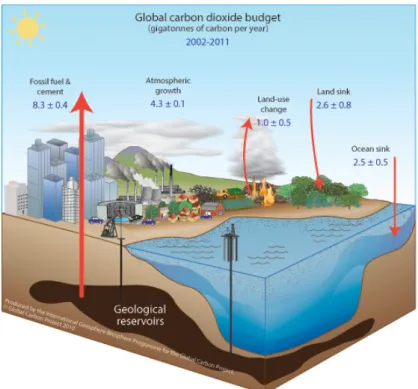
The global carbon budget averaged over the last decade (2002–2011) is shown in Fig. 1. For this time period, 89 % of
the total emissions (EFF+ ELUC) were caused by fossil fuel
combustion and cement production, and 11 % by land-use change. The total emissions were partitioned among the at-mosphere (46 %), ocean (27 %) and land (28 %). All com-ponents except land-use change emissions have grown since 1959 (Figs. 2 and 3), with important interannual variability in the atmospheric growth rate caused primarily by variability
in the land CO2sink (Fig. 3), and some decadal variability in
all terms (Table 4).
Global CO2emissions from fossil fuel combustion and
ce-ment production have increased every decade from an
aver-age of 3.1 ± 0.2 PgC yr−1 in the 1960s to 8.3 ± 0.4 PgC yr−1
during 2002–2011 (Table 4). The growth rate in these emis-sions decreased between the 1960s and the 1990s, from
4.5 % yr−1 in the 1960s, 2.9 % yr−1in the 1970s, 1.9 % yr−1
in the 1980s, 1.0 % yr−1 in the 1990s, and increased again
since year 2000 at an average of 3.1 % yr−1. In contrast,
CO2emissions from LUC have remained constant at around
1.5 ± 0.5 PgC yr−1during 1960–1999, and decreased to 1.0 ±
0.5 PgC yr−1since year 2000. The decreased emissions from
LUC since 2000 is also reproduced by the DGVMs (Fig. 5).
The growth rate in atmospheric CO2increased from 1.7 ±
0.1 PgC yr−1in the 1960s to 4.3 ± 0.1 PgC yr−1during 2002–
2011 with important decadal variations (Table 4). The ocean
CO2 sink increased from 1.2 ± 0.5 PgC yr−1 in the 1960s
to 2.5 ± 0.5 PgC yr−1 during 2002–2011, with decadal
vari-ations of the order of a few tenths of PgC yr−1. The low
uptake anomaly around year 2000 originates from multi-ple regions in all models (west Equatorial Pacific, Southern Ocean and North Atlantic), and is caused by climate
variabil-ity. The land CO2 sink increased from 1.7 ± 0.8 PgC yr−1 in
the 1960s to 2.6 ± 0.8 PgC yr−1during 2002–2011, with
im-portant decadal variations of 1–2 PgC yr−1. The high uptake
anomaly around year 1991 is thought to be caused by the
effect of the volcanic eruption of Mount Pinatubo, and is
re-produced in some of the models only, but not by the model average (Fig. 5).
Figure 1.Schematic representation of the overall perturbation of the global carbon cycle caused by anthropogenic activities, averaged glob-ally for the decade 2002–2011. The arrows represent emission from fossil fuel burning and cement production; emissions from deforestation and other land-use change; and the carbon sinks from the atmosphere to the ocean and land reservoirs. The annual growth of carbon diox-ide in the atmosphere is also shown. All fluxes are in units of PgC yr−1, with uncertainties reported as ±1 sigma (68 % confidence that the
real value lies within the given interval) as described in the text. This Figure is an update of one prepared by the International Geosphere Biosphere Programme for the GCP, first presented in Le Qu´er´e (2009).
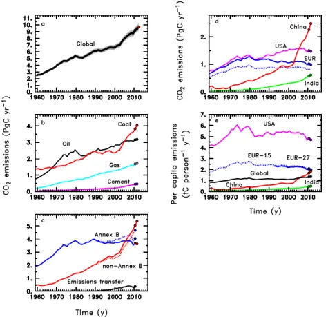
3.2 Global carbon budget for year 2011 and emissions projection for 2012
Global CO2 emissions from fossil fuel combustion and
ce-ment production reached 9.5 ± 0.5 PgC in 2011 (Fig. 4; see also Peters et al., 2013). The total emissions in 2011 were dis-tributed among coal (43 %), oil (34 %), gas (18 %), cement (4.9 %) and gas flaring (0.7 %). These first four categories increased by 5.4, 0.7, 2.2, and 2.7 % respectively over the previous year, without enough data to calculate the change for gas flaring. Using Eq. (5), we estimate that global CO2 emissions in 2012 will reach 9.7 ± 0.5 PgC, or 2.6 % above 2011 levels (likely range of 1.9–3.5; Peters et al., 2013), and that emissions in 2012 will thus be 58 % above emissions in 1990. The expected value is computed using the world GDP projection of 3.3 % made by the IMF (October 2012)
and a growth rate for IFF of −0.7 %, which is the average
from the previous 10 yr. The uncertainty range is based on 0.2 % for GDP growth (the range in IMF estimates published in January, April, July, and October 2012) and the range in
IFFdue to short term trends of −0.1 % yr−1(2007–2011) and
medium term trends of −1.2 % yr−1 (1990–2011); the
com-bined uncertainty range is therefore 1.9 % (3.3–1.2–0.2) and
3.5 % (3.3–0.1+ 0.2). Projections made for the 2009, 2010,
and 2011 CO2budget compared well to the actual CO2
emis-sions for that year (Table 5) and were useful to capture the current state of the fossil fuel emissions.
In 2011, global CO2 emissions were dominated by
emis-sions from China (28 % in 2011), the USA (16 %), the EU (27 member states; 11 %), and India (7 %). The per-capita
CO2 emissions in 2011 were 1.4 tC person−1yr−1 for the
globe, and 4.7, 1.8, 2.0 and 0.5 tC person−1yr−1for the USA,
China, the EU and India, respectively (Fig. 4e).
Territorial-based emissions in Annex B countries have re-mained stable from 1990–2000, while consumption-based
emissions have grown at 0.5 % yr−1 (Fig. 4c). In
non-Annex B countries territorial-based emissions have grown at
4.4 % yr−1, while consumption-based emissions have grown
at 4.0 % yr−1. In 1990, 65 % of global territorial-based
emis-sions were emitted in Annex B countries, while in 2010 this had reduced to 42 %. In terms of consumption-based emissions this split was 66 % in 1990 and 46 % in 2010.
The difference between territorial-based and
consumption-based emissions (the net emission transfer via international trade) from non-Annex B to Annex B countries has
in-creased from 0.04 PgC yr−1 in 1990 to 0.38 PgC in 2010
(Fig. 4), with an average annual growth rate of 9 % yr−1.
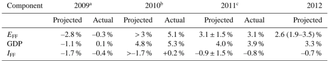
Table 5.Actual CO2emissions from fossil fuel combustion and cement production (EFF) compared to projections made the previous year
based on world GDP and the fossil fuel intensity of GDP (IFF). The “Actual” values and the “Projected” value for 2012 refer to those presented
in this paper.
Component 2009a 2010b 2011c 2012
Projected Actual Projected Actual Projected Actual Projected
EFF –2.8 % –0.3 % > 3 % 5.1 % 3.1 ± 1.5 % 3.1 % 2.6 (1.9–3.5) %
GDP –1.1 % 0.1 % 4.8 % 5.3 % 4.0 % 3.9 % 3.3 %
IFF –1.7 % –0.4 % >–1.7 % +0.2 % –0.9 ± 1.5 % –0.8 % –0.7 %
aLe Qu´er´e et al. (2009),bFriedlingstein et al. (2010),cPeters et al. (2013)
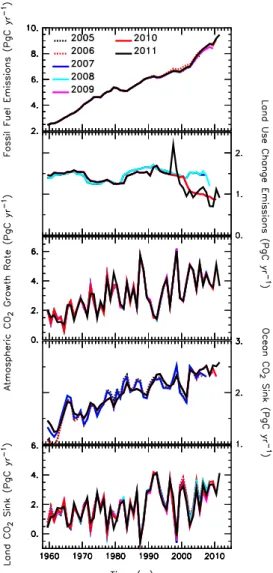
47 1 2 Fig. 2 3 4
Figure 2.Combined components of the global carbon budget illus-trated in Fig. 1 as a function of time, for (top) emissions from fossil fuel combustion and cement production (EFF; grey) and emissions
from land-use change (ELUC; brown), and (bottom) their
partition-ing among the atmosphere (GATM; light blue), land (SLAND; green)
and ocean (SOCEAN; dark blue). All time series are in PgC yr−1.
Land-use change emissions include management–climate interac-tions from year 1997 onwards, where the line changes from dashed to full.
1990–2008 compares with the emission reduction of 0.2 PgC in Annex B countries. These results clearly show a grow-ing net emission transfer via international trade from non-Annex B to non-Annex B countries. In 2010, the biggest emit-ters from a territorial-based perspective were China (26 %), USA (17 %), EU (12 %), and India (7 %), while the biggest emitters from a consumption-based perspective were China (22 %), USA (18 %), EU (15 %), and India (6 %).
Global CO2 emissions from Land-Use Change activities
were 0.9 ± 0.5 PgC in 2011, with the decrease of 0.2 PgC yr−1
from the year 2010 estimate based on satellite-detected fire activity.
Atmospheric CO2 growth rate was 3.6 ± 0.2 PgC in 2011
(1.69 ± 0.09 ppm; Fig. 3). This is slightly below the 2000–
2009 average of 4.0 ± 0.1 PgC yr−1, though the interannual
variability in atmospheric growth rate is large.
The ocean CO2 sink was 2.7 ± 0.5 PgC yr−1 in 2011, a
slight increase compared to the sink of 2.5 ± 0.5 PgC yr−1in
2010 and 2.4 ± 0.5 PgC yr−1in 2000–2009 (Fig. 3). All
mod-els suggest that the ocean CO2sink in 2011 was greater than
the 2010 sink.
The terrestrial CO2 sink calculated as the residual from
the carbon budget was 4.1 ± 0.9 PgC in 2011, well above the
2.7 ± 0.9 PgC in 2010 and 2.4 ± 0.9 PgC yr−1 in 2000–2009
(Fig. 3). This large sink is consistent with enhanced CO2sink
during the wet and cold conditions associated with the strong La Ni˜na condition that started in the middle of 2010 and ended in March 2012, as discussed for previous events (Keel-ing et al., 1995; Peylin et al., 2005). Results from DGVMs are available to year 2010 only (Fig. 5).
4 Discussion
Each year when the global carbon budget is published, each component for all previous years is updated to take into ac-count corrections that are due to further scrutiny and verifi-cation of the underlying data in the primary input datasets (Fig. 6). The updates have generally been relatively small and generally focused on the most recent past years, ex-cept for LUC between 2008 and 2009 when LUC emissions
were revised downwards by 0.56 PgC yr−1, and after 1997
for this budget where we introduced an estimate of interan-nual variability from management–climate interactions. The
2008/2009 revision was the result of the release of FAO 2010,
which contained a major update to forest cover change for the period 2000–2005 and provided the data for the
follow-ing 5 yr to 2010. Updates were at most 0.24 PgC yr−1for the
fossil fuel and cement emissions, 0.19 PgC yr−1for the
atmo-spheric growth rate, 0.20 PgC yr−1 for the ocean CO
2 sink.
The update for the residual land CO2 sink was also large,
with maximum value of 0.71 PgC yr−1, directly reflecting the
revision in other terms of the budget. Likewise, the land sink estimated by DGVMs has also reflected the increasing avail-ability of model output to do these calculations.
Our capacity to separate the CO2budget components can