HAL Id: halshs-01136848
https://halshs.archives-ouvertes.fr/halshs-01136848
Submitted on 31 Jan 2017
HAL is a multi-disciplinary open access
archive for the deposit and dissemination of sci-entific research documents, whether they are pub-lished or not. The documents may come from teaching and research institutions in France or abroad, or from public or private research centers.
L’archive ouverte pluridisciplinaire HAL, est destinée au dépôt et à la diffusion de documents scientifiques de niveau recherche, publiés ou non, émanant des établissements d’enseignement et de recherche français ou étrangers, des laboratoires publics ou privés.
approach
Sébastien Oliveau
To cite this version:
Sébastien Oliveau. Peri-Urbanisation in Tamil Nadu : A quantitative approach. pp.92, 2005, CSH Occasional Paper, ISSN- 0972 - 3579. �halshs-01136848�
N o . 15
2 0 0 5
C S H O c c a s i o n a l P a p e r
P
ERIURBANISATION
IN
T
AMIL
N
ADU
:
a quantitative approach
Sébastien Oliveau
THE EDITORIAL ADVISORY BOARD FOR THE CSH OCCASIONAL PAPERS
- Balveer ARORA, Centre for Political Studies, Jawaharlal Nehru University, New Delhi
- Rajeev BHARGAVA, Centre for the Study of Developing Societies, Delhi
- Partha CHATTERJEE, Centre for Studies in Social Sciences, Kolkata - Jean DREZE, Govind Ballabh Pant Social Science Institute,
Allahabad
- Jean-Claude GALEY, Ecole des Hautes Etudes en Sciences Sociales, Centre for Indian and South Asian Studies, Paris
- Archana GHOSH, Institute of Social Sciences, Kolkata
- Michel GRIFFON, Centre de Coopération Internationale en Recherche Agronomique pour le Développement, Nogent-sur-Marne - Christophe JAFFRELOT, Centre National de la Recherche Scientifique, Centre for International Studies and Research, Paris - S. JANAKARAJAN, Madras Institute of Development Studies,
Chennai
- Harish KAPUR, European Institute, New Delhi
- Amitabh KUNDU, Centre for the Study of Regional Development, School of Social Sciences, Jawaharlal Nehru University, New Delhi - Amitabh MATTOO, University of Jammu
- C. Raja MOHAN, Strategic Affairs, Indian Express, New Delhi - Jean-Luc RACINE, Centre National de la Recherche Scientifique,
Centre for Indian and South Asian Studies, Paris
- R. RADHAKRISHNA, Indira Gandhi Institute of Development Research, Mumbai
- P. R. SHUKLA, Indian Institute of Management, Ahmedabad - Joël RUET, DESTIN, London School of Economics
- Gérard TOFFIN, Centre National de la Recherche Scientifique, Research Unit : Environment, Society and Culture in Himalayas, Paris - Patricia UBEROI, Institute of Economic Growth, Delhi
- Anne VAUGIER-CHATTERJEE, Political Affairs, Delegation of the European Commission in India, Bhutan, Maldives, Nepal and Sri Lanka, New Delhi.
P
ERIURBANISATION
IN
T
AMIL
N
ADU
:
a quantitative approach
Sébastien Oliveau
December 2005
Centre de Sciences Humaines (Centre for Social Sciences): Created in New
Delhi in 1990, the CSH, like its counterpart in Pondicherry (Institut Français
de Pondichéry), is part of the network of research centres of the French
Ministry of Foreign Affairs. The Centre’s research work is primarily oriented towards the study of issues concerning the contemporary dynamics of development in India and South Asia. The activities of the Centre are focused on four main themes, namely: Economic transition and sustainable
development; Regional dynamics in South Asia and international relations; Political dynamics, institutional set-up and social transformations; Urban dynamics.
[Centre de Sciences Humaines, 2, Aurangzeb Road, New Delhi 110 011 Tel.: (91 11) 30 41 00 70 Fax: (91 11) 30 41 00 79
Email: [email protected] – Website: http://www.csh-delhi.com]
Institut Français de Pondichéry (French Institute of Pondicherry): Created in
1955, the IFP is a multidisciplinary research and advanced educational institute. Major research works are focussing on Sanskrit and Tamil languages and literatures (in close collaboration with the Ecole Française d’Extrême-Orient), ecosystems, biodiversity and sustainibility, dynamics of population and socio-economic development.
Institut Français de Pondichéry,
11 Saint Louis Street, PB 33, Pondicherry 605 001 Tel. : (91) 413 2334168 Fax : (91) 413 2339534 http://www.infpindia.org
© Centre de Sciences Humaines, 2005
All rights reserved. No part of this publication may be reproduced or
transmitted, in any form or means, without prior permission of the author or the publisher
Published by Raman Naahar, Rajdhani Art Press, Tel. : 98102 45301
The opinions expressed in these papers are solely those of the author(s).
ABOUT THE AUTHOR
Sébastien Oliveau (Sé[email protected]
http://www.geodemo.net) is associate professor at the University of Provence, France. He has his PhD from University Paris 1 Panthéon-Sorbonne, and was a scholar at the French Institute of Pondicherry (IFP). He has specialised in GIS and Geostatistics. His work focuses on spatial dimensions of social change in South India. In 2003 he edited an online atlas of South India which was published in the European journal of Geography Cybergeo (http:/ /www.cybergeo.presse.fr).
ABOUT THIS OCCASIONAL PAPER
This Occasional paper is the second volume of a series of three on
Peri-urban dynamics. The first volume proposed a review of
concepts and general issues (CSH Occasional Paper No. 14, edited by Véronique Dupont) and the third volume will present case studies in Chennai, Hyderabad and Mumbai.
ACKNOWLEDGEMENTS
First and foremost, I have to thank Christophe Z.Guilmoto for constantly providing valuable advice, guidance and support since 1998. Through him, I thank all the colleagues of the different projects (Population and Space, South Indian Fertility Project, Espace et Mesure en Inde du Sud) I worked with.
This Occasional Paper is a follow-up to the presentation made at the international workshop on “Peri-urban Dynamics: Population, Habitat and Environment on the Peripheries of Large Indian Metropolises” held in Delhi on 25 and 26 August 2004. I am indebted to Véronique Dupont, Head of the Centre des Sciences Humaines (CSH, New-Delhi - India) who invited me to this workshop and gave me the opportunity to publish an extended version of the work presented at the workshop. At the CSH, I am thankful to Attreyee Roy Chowdhury, for her patience, and Bertrand Lefebvre for his help. The attentive reading by my two referees helped me to improve this paper. However, the remaining inaccuracies are mine.
This paper restates some of the results of a doctoral thesis submitted to the University Of Paris 1 Panthéon-Sorbonne on the spatial dimensions of modernisation in Tamil Nadu. I should first express my gratitude to Denise Pumain, who agreed to supervise my Ph.D., and all the Geographie-cités team (CNRS, Paris - France). The French Institute of Pondicherry (Population & Space Programme) provided funding, office space and staff support for my work. It was also sponsored by the Laboratoire Population-Environnement-Développement (IRD, Marseille - France), the French ministry of education and research, the French ministry of foreign affairs. The University of Madras (Chennai - India) welcomed me in the French and Geography Department.
Last, but not least, I wish to thank my family, and especially Pauline, who always supported me.
CONTENTS
INTRODUCTION 1
A. Cities and Rural Areas 3
1. Dichotomy or Continuum? 4
a) Non-acceptance of antagonism 4
b) Multiplicity of rural areas 8
2. Defining the City 10
a) Cities and rural areas, agriculture and services 12 b) Redefining the city in Tamil Nadu 13
3. From Towns to Rural Areas 22
a) Towns and rural areas: core and periphery? 23 b) Distance: “The first attribute of a spatial system” 26
c) Choosing one’s distance 31
B. Urban Influences in Tamil Nadu 35
1. A Statistical Approach to Urban Influence 37
a) Going step by step 39
b) Playing with hypothesis: Interpreting the Graph 43 c) A step-by-step approach to modernisation 45 2. The Effect of Different Types of Towns 49 a) The importance of the “one lakh cities” 49 b) Urban status, a reflection of urban hierarchies 56
c) Economic functions of towns 58
d) At the top: urban agglomerations and 61 strong services sector
e) Periurbanisation 64
3. Accessibility of towns 67
a) Roads, an avenue of modernisation 67 b) The train, an extension of the town 71 c) Modernisation and access to town 75
CONCLUSION 81
LIST OF TABLES
Table 1 Classification of 225 Towns and 18
Urban Agglomerations in Tamil Nadu
Table 2 Status and Population of Towns in Tamil Nadu 18
Table 3 Types of Towns in Tamil Nadu 21
(absolute numbers and percentage)
Table 4 Administrative Status and Urban Functions 21
in Tamil Nadu
Table 5 Differences in distance according to the point 33 of reference in the town
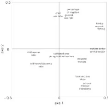
Table 6 Presentation of the axes of the principal 33
components analysis
Table 7 Correlation of variables with the two principal 34 axes of the analysis.
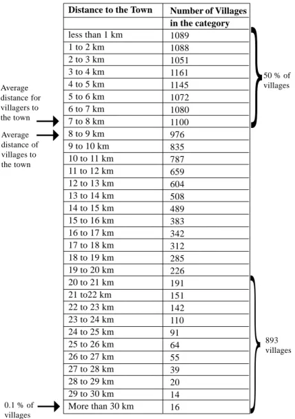
Table 8 Number of villages for each step of distance. 40
Table 9 Correlation between modernisation factors and 47 different functions of the distance to the town
Table 10 Average level of village modernisation around 54 towns according to the class of town
Table 11 village modernisation and distance to town 59
according to the urban economic function.
Table 12 A categorywise approach to the modernisation 61 of villages according to the type of town.
Table 13 Relation between distance to road and 71
village modernisation
Table 14 A comparison of the coefficient of determinations 77 of different fittings of the modernisation index.
Table 15 Modernisation level of villages according to 78 their geographical location.
LIST OF FIGURES
Figure 1 Different definitions of urban 11 Figure 2 Should the measurement be taken from 32
the centre or from the town’s border ?
Figure 3 Projection of axes 1 and 2 of the principal 34 components analysis
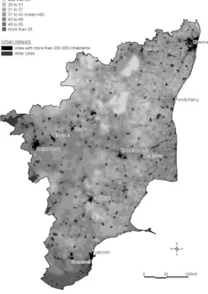
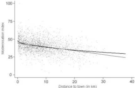
Figure 4 Modernisation of rural areas in Tamil Nadu 35 Figure 5 Modernisation of the village and the distance 38
to the town (square root function)
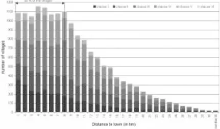
Figure 6 Number of villages per step of distance 42 (differentiated in relation to the urban population) Figure 7 Village modernisation and distance to town 43
(seen as a cross-section)
Figure 8 Variation of indices constituting the 48 modernisation index according to the distance
to the town
Figure 9 Modernisation and the distance to the town 55 according to the population of the nearest town. Figure 10 village modernisation and distance to town,
according to its urban status. 58 Figure 11 village modernisation and distance to town 60
according to the urban economic function
Figure 12 village modernisation and distance to town 63 according to their economic orientation
and urban status.
Figure 13 From the urban to the rural in Tamil Nadu: 66 differentiated spaces.
Figure 14 village modernisation and distance to town 69 according to the distance to the road network.
Figure 15 village modernisation and distance to town 71 according to the type road
Figure 16 village modernisation and distance to rail 73 network.
Figure 17 village modernisation and distance to town 74 according to the distance to the rail network.
Figure 18 Distance to the town and accessibility: 79 another view of the periurbain area
INTRODUCTION1
Our study of periurbanisation is in the nature of a general regional analysis. We believe that the differences observed at the regional level are the result of various types of changes. One of these changes, namely urban expansion, is of a singular nature and is particularly important as much for its social as for its spatial dimension. If urban expansion is seen as a dynamic phenomenon when analysing the relationship between the cities and the countryside, it can be interpreted as a phenomenon responsible for innovation (Berry, 1973). In a synchronic study of urban expansion where its kinetic dimension is not taken into account, it is preferable to use a centre-periphery model. Such a model envisages a social or spatial organisation (and in geography, often as the transfer of the first to the second) where the centre dominates the periphery. Periurban space is then said to be dominated by the city, while rural space is not (or no longer) dominated by it. Periurbanisation can hence be understood as a specific phase of urban expansion. It is then possible to discern the social dimension or, to put it briefly, the transformation of the habitus and modes of production as well as the geographical dimension seen as the projection of social issues in space. This projection is directly visible while studying the landscape, particularly in the changes in the settlement pattern that it brings about, but also indirectly while analysing the characteristics of the population units. What
1 This paper seeks to convey a view of periurbanisation based on French documentation and experiences. French geographers have shown a great deal of interest in the relationship between cities and rural areas from the early twentieth century and have faced the problem of periurbanisation as far back as the 1950s. Furthermore, the population in France is relatively concentrated around well-defined cities, a situation very similar to India’s, especially in Tamil Nadu. Finally, l’INSEE (National Institute for Statistics and Economic Studies, Paris - France) has done significant work in this field and has contributed to the classification of rural areas in France in order to highlight their diversity.
particularly interests us is the latter dimension, which can be understood through statistical and cartographic analyses.
However, urban expansion does not systematically give rise to the phenomena of periurbanisation. Thus, there may be instances where there is a continuous spread of the urban population (suburbs), as well as the spread of urban ideology to rural areas, which is often described as modernisation, but which could also be called social urbanisation.
Thus the structure of suburbanisation differentiates it from periurbanisation. Similarly, rural entities assume urban characteristics like the development of secondary (industry) and especially tertiary (services) activities, an increase in the level of education and the appearance of new services and businesses. More inhabitants have contacts with the city (due to greater accessibility and mobility). The major difference between suburbs and periurban villages lies in their physical links with the city. Suburbs are the continuation of the built-up area from the main city and tend to administratively merge with the city in the long run, whereas periurban spaces are still physically separated from the city by agricultural land and /or natural open spaces (there is no continuity with the build-up area of the city).
Finally, the phenomena of change often affects rural non-periurban spaces or, in other words, they may transform the way of life even though there may not be any change in the general (spatial or architectural for example) characteristics of the villages. Thus, the advent of the media in the form of newspapers, radio or television changes the villagers’ perception without necessarily changing the village itself. Furthermore, there is no change in the access to the city. We thus find ourselves in the presence of modernisation, whose geographical consequences are not necessarily visible or are too minor to be taken into consideration. Regarding this last point, we find that when a change affects society as a whole, with the same
force and at the same time, it does not lead to spatial differentiation, as the existing equilibrium is not disturbed. So, though it is easy to differentiate between the suburbs and periurban spaces, the difference between periurbanisation and the modernisation of the rural environment is much more blurred.
It is from this point of view that we have conducted this study. This paper is divided into two main parts. The first is more concerned with methodology; it places our approach in the right perspective and describes the tools used to obtain the results presented in the second part, which shows how the city exerts its influence on villages, first by emphasising the relationship between cities and rural areas and then by drawing attention to the real dimension of periurbanisation. Finally, we will question the role of accessibility, which will enable us to propose in our conclusion a more refined model of the periurban setup.
A. Cities and Rural Areas
The study of the relationship between cities and rural areas in France can be traced back to the writings of Georges Chabot in 1931 on “zones influenced by cities” (Dugrand, 1963). Studies on this subject increased after World War II with research being conducted in the different regions of France (see, for example, Kayser, 1960, Dugrand, 1963).
In India too, there have been a number of studies on cities and rural areas (see, for example, Berry & Rao, 1968). However, there was a decline in the 1980s. Sopher’s book (1980) constitutes the high point of this research, especially the chapter by Sharma (1980) focusing on the relationship between the major cities and the rural hinterland in eastern Gujarat and north-west Andhra Pradesh. Kundu offers an explanation for this decline in his work on the links between cities and rural areas; he says that since
researchers were not able to find zones of influence around Indian cities as obvious as those seen in the West, they gave up this field of study (Kundu, 1992). It is also possible that the tools and data available at that time did not allow them to proceed further with their investigations. The development of information technology, which has made it easier to process large quantities of data, and the availability of a wider variety of data, have given rise to new research in this field. The most recent example is the exploration of different forms of periurbanisation by Kundu and others with the help of data from NCAER (National Council of Applied Economic Research) and census reports (Kundu et al., 2002).2
1. Dichotomy or Continuum?
The city as the home of modernity is the opposite of the village, which stands for tradition. At least in India, this was the view held by Gandhi, because for him the city was the symbol of colonisation and he believed that the “real” India lived in its villages. Ambedkar, on the contrary, described the village as “a sink of localism and a den of ignorance and narrow mindedness and communalism” (Ambedkar, 1948). The cliché persists even today. But this opposition is not fiction for “perceptive experience makes the difference between urban and rural environments very obvious” (Schmitt, Gofette-Nagot, 2000: 42). That is precisely why these two categories are so clearly differentiated in our interpretation of this phenomenon.
a) Non-acceptance of antagonism
It is generally acknowledged that the city is a centre of innovation bringing together rare services (Charrier, 1998: 34-35; Guillain, Huriot, 2000). We may refer to Bairoch’s explanatory model to understand this phenomenon: when the population of a place 2 We have already pointed out the limitations of this approach in Guilmoto, Oliveau et
increases, the absolute number of individuals engaged in non-agricultural activities goes up. This increase leads to a rise in the specialisation and diversification of activities (Bairoch, 1985: 47). This model is in accordance with Christaller’s theory of central places, which explains the presence of an urban hierarchy by differentiating functional levels (Christaller, 1933). This diversity is therefore one of the elements in the innovative power of cities as compared to villages. We may add the role of density and the greater freedom enjoyed by individuals.
Innovators need to interact, and to interact they must meet. In addition, interaction between individuals depends on their proximity (Pini, 1992). So the greater the density, the more the general proximity. The increase in density is thus accompanied by a greater probability of interaction between individuals (Pumain & Robic, 1996). Since there is more density in cities, there is also more interaction (Pumain & Saint Julien, 2001). This is the “density effect” described by Guillain and Huriot (2000).
Moreover, change is often the result of sharing different experiences and therefore requires social, cultural and/or economic diversity. Almost by definition, the city is a place where there is not only economic diversity (Pumain, 1992a), but also social and cultural diversity, because it is a place where there is relative freedom.
As a matter of fact, and this is especially true of India, the city is a place where there is least social pressure and this allows individuals to act with fewer constraints, finding themselves paradoxically sheltered by the ‘group within the crowd’. They can free themselves from some of the established rules of behaviour (Srinivas, 1996a) as they are sheltered from the critical eyes of others and from what could be called the “village effect”. Once behaviour is freed from the restraints imposed by tradition, it can change more easily. This aspect of the city encourages and
attracts the forces of social change and individuals whose inclination is not to conform to the norm.3
There is thus a tendency to oppose these two categories (city/ modernity and rural/tradition) according to a binary logic that simplifies analysis. The antagonism between a modern urban object and a rural object, which is not modern, is stressed by Kundu et al. (2002). They stress that there is an absence of continuum in the space surrounding urban centres and defend the idea of a dichotomy by underlining the fact that socio-economic indicators do not decrease gradually from the cities to the surrounding countryside.
As for us, we prefer to interpret these results as a sign of non-linear continuity. If the indicators decrease abruptly, it is because cities do not have a significant disseminative capacity. Nevertheless, the continuity cannot be denied. This continuity is one of the reasons why the dichotomous approach opposing the city to the country in black and white terms has progressively lost its significance and has now been practically abandoned.4 This abandonment must be considered in the context of changes which may be different but leads to the same conclusions, as indicated by studies in the developing countries and the so-called Western countries (on this subject, see Hugo et al., 2003). The former have brought to the forefront the close relations that rural migrants in cities continue to maintain with their native villages. All studies on migrants in India confirm this, whether it
3 It may also be pointed out that the bigger the city, the more migrants it attracts from afar who make the population more heterogeneous.
4 It is interesting to note that the ancient Indian texts say that the city and the countryside are like two points of a continuum (Kundu, 1999 – on the basis of B.D. Chattopadhaya’s book (1997), “The City in Early India: Perspectives from Texts”, Studies in History, Jawaharlal Nehru University, New Delhi).
is the rural areas of Karnataka (Racine 1994) or the homeless population of Delhi (Dupont, 1999). The latter even go so far as to recreate their villages in the slums of the metropolis, “importing” their rural value systems into the heart of the world’s largest metropolises, Bombay’s Dharavi slum being an excellent example (Saglio-Yatzimirsky, 2002). Besides, the inhabitants of cities and rural areas in developing countries move from one to the other and use the resources provided by these spaces, often keeping “one foot in and one foot out”, as Chaléard and Dubresson (1989) have said about Abidjan, the capital of Ivory Coast. Ramachandran (1989: 99), whose outlook is a more cultural one, emphasises the continuity between urban and rural spaces. India being a country that is socially stratified by religion (and jati), ethnic groups and linguistic differences, the pattern of living is more closely linked with the social group(s) to which a person belongs than with the place where he/she lives. Social practices (extended families, rules regarding marriage and commensalism, etc.) do not change (or change very little) irrespective of the place or the size of the population unit. Even though the city allows much more freedom, many values remain common to the village and the city.
The introduction of rural customs into cities in the developing countries is comparable to the extension of urban culture to rural areas in the western countries. In the latter, the development of mass media has spread urban ideas to the rural world, thus effacing the major part of the differences between the inhabitants of these two spaces. Today, some people in France would like to eliminate the differences between the city and the countryside, considering that all lifestyles are similar to the urban lifestyle. However, this typically western attitude needs to be qualified. Even if all patterns of living become alike, there would still be differences whose importance should not be underestimated, because people do not live in the same way in a village in central
France as in the central districts of Paris, irrespective of the social stratum to which they belong.
The same processes are at work in the North and in the South and the media play the same role (depending, of course, on their presence in these areas). Urban and rural cultures influence each other and it becomes clear that proximity makes this exchange easier. Besides, this adds force to Chaléard’s and Dubresson’s observation (1999: 12) in their introduction to Villes et campagnes
dans les pays du Sud: “The most dynamic rural areas are often
those that are the most closely connected with cities, while enclosed spaces or more distant urban agglomerations are generally those that are the most affected by poverty and depopulation.” As these writers suggest, it is advisable to give up this dichotomous view and alleged antagonism to affirm the continuity of the two spaces, retaining the terms urban and rural only “for the sake of linguistic convenience [to describe] the two extremes of a gradient representing the intensity of the change” (Auriac, Rey, 1998: 30), because the distinction between these two types of population is useful (Pumain, 1992a: 445).
b) Multiplicity of rural areas
It therefore follows that one cannot have the countryside on one side and the city on the other in opposition to each other. There are in fact rural areas that are economically and socially heterogeneous within the same region and geographers have made no mistake about it. The multitude of terms that exist to describe these different phenomena says it all. Thus, there are several words to describe the zones around cities and those lying further away: “hinterland” is used in one international version5 and “umland” in another (though both are derived from German, um means around while
hinter means behind)6. The term “decay” is more technical and
used in the field of spatial analysis.
If there are so many terms, it is because the grasp of the phenomenon and of its numerous forms can vary in space and change with time. The richness of the terminology reflects the numerous and multiple patterns of settlement that are found, urging each writer to qualify this notion. The most recent studies on the western world use new terms like “periurbanisation”7 which seeks to describe the urbanisation of the countryside on the periphery of cities. The term « rurbanisation » is also used to emphasise the social transformation of rural areas, that is to say their integration into the urban value system (a phenomenon that is still very western but is gradually spreading to the societies of the South), mainly due to the migration of the urban population to rural areas as a return to one’s roots or migration to more salubrious lands. The term “counterurbanization” has been proposed to describe this phenomenon of city-dwellers settling down in the countryside. We will now concentrate on the phenomenon of periurbanisation and focus on the view proposed by INSEE through its nomenclature of French communes. This nomenclature introduces a geographical dimension in the classification by distinguishing between two types of spaces: “spaces that are predominantly urban” and “spaces that are predominantly rural”. Thus predominantly urban spaces – divided into an urban area, an urban pole, a periurban ring, multi-polarised communes and periurban communes – are opposed to predominantly rural spaces, where it is possible to make a distinction between rural areas where the urban influence is negligible, rural poles, their periphery and finally isolated rural areas (Hilal, Schmitt, 1997). The
6 Kundu (1992: 101) remarks that the two terms are sometimes interchangeable. 7 The periurban concept itself has several interpretations. As Jean & Calenge (1997: 391) remind us, “each writer stresses on one aspect, which results in a variable terminology, reflecting the vagueness of space.”
geographical dimension is reintroduced in this manner in the socio-economic analysis of spaces.
This very precise division reminds us of an essential element in the study of the relationship between cities and rural areas: the dichotomy is artificial, the division is not very clear and the rural-urban continuum remains. “It is indispensable to differentiate rural spaces according to their distance from the city and the intensity of their relations with the latter. In fact, being close to the city allows the rural areas to partly benefit from the advantages of the city.” (Goffette-Nagot, Schmitt, 1998: 175).
It is however advisable to point out that rural space is always defined as opposed to the city: “defining space amounts in this case to agreeing on a definition of what is urban” (Schmitt, Gofette-Nagot; 2000: 43). The definition of urban generally forms the centre of the study and rural is defined as its opposite (Hugo et al., 2003). Though this scientific attitude is sometimes criticised (Thomsin, 2001), it is justifiable and it is difficult to get rid of it.
If we look at it from a historical perspective, rural space seems to be the foundation on which cities developed. So there must be an earlier undefined space from which the city, a new geographical object, emerged. Every city is born of a village8. The rural precedes the urban9. However, this new object stands out and is the subject of a special definition.
2. Defining the City
It therefore seems necessary to propose a definition for the urban fact before proceeding any further. But though the city may be “a fact that cannot be ignored, an indisputable proof, one does not 8 There are certainly cities that were created ex nihilo (Chandigarh is a good example in India), but these cities appear nonetheless in a space that was earlier classified as rural. 9 This is shown for example by Champakalakshmi (1996) with reference to South India.
know how to define it, at least completely, that is to say in a manner encompassing all the manifestations of the term, and nothing but these manifestations, and that this definition should be acceptable to all.” (Derycke et al., 1996: 324).
The impossibility of finding a single definition of the city has been pointed out many times (Pumain, Robic, 1996; Beguin, 1996) and is due mainly to its universal character. The city is present everywhere and each society builds it in its own way. This universal character has made it multiform. To describe it, we must use criteria that are simultaneously social, demographic, historical and spatial (Pumain, 1994). This multiplicity of criteria rules out any permanent definition. As Le Gleau, et al. wrote about Europe, “cities are objects that are too rich and too diverse for only one definition or a single concept to be able to describe them” (Le Gleau, et al., 1996: 10).
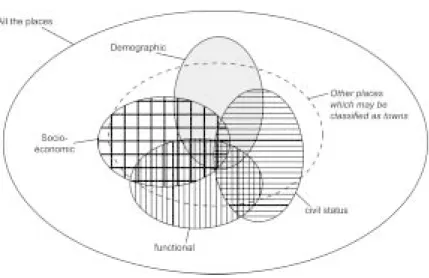
Figure 1 : Different definitions of urban10
(according to Moriconi-Ebrard, 1994: 52)
10 For definitions of the city, we will refer to Bairoch (1985: 29) who estimates that by taking up “systematically all the criteria suggested by various writers, we may probably reach 25 to 30 [definitions].”
That is why Moriconi-Ebrard (1994: 52) suggests “the lowest common denominator” of urbanity at the crossroads of different approaches (zone shown in black in Figure 1). He tries to explain the complexity of the phenomenon by proposing a definition that is intentionally too restrictive because his approach has a precise aim, namely to arrive at an international comparison. In the case of non-global approaches, we must redefine our object. It is necessary to take into account the local specificity of the urban fact, particularly the way the city is perceived and experienced. For this, we must envisage different definitions of urban areas before choosing the ones that are most suited to our study. It is advisable to think of what makes the city what it is in general and then compare this definition with what the city represents in the space that interests us, namely Tamil Nadu.
a) Cities and rural areas, agriculture and services
The first cities were born when man became capable of producing an agricultural surplus that enabled other men to devote themselves to other productive activities (economic, political or spiritual). These new forms of production called for the exchange of products with other units of population. This led to the creation of market-places, which sometimes expanded to become centres of exchange, as distinguished from areas of agricultural production (Bairoch, 1985; regarding South India: Champalakshmi, 1996).
This hypothesis on the emergence of the first cities has moulded our way of looking at the urban-rural opposition and the town/city is often defined as a living space where the industrial and services sectors are over-represented. Besides, this definition very often corresponds to reality, and if we were to “look for a purely economic definition, the city would be a place the majority of whose inhabitants earn their living from industry or trade, and not from agriculture. […] It is necessary to add one more criterion: the variety of practical knowledge and professions.” (Weber, 1982: 18).
This definition is undoubtedly relative and agricultural activity may still represent a large part of urban activity, as was the case until the second half of the 20th century in Europe or even today in many towns all over the world (Charrier, 1988). On the other hand, there are instances of villages where agricultural activity is almost absent. Rural industries have existed from ancient times in Europe as well as in India and activities like tourism and teleworking provide new opportunities today in rural areas. The first interpretation of the city as a place having the least agricultural activity is therefore frequently complemented by another trait, namely the strong presence of rare activities. Actually, what differentiates the city from the countryside is the presence of specific services, commercial or otherwise (formerly the postal service and later the telephone before its spread to rural areas, some administrative services like tax collection, trade in luxury goods, etc.). What constitutes the singularity of urban areas is also used to classify cities among themselves and is correlated to the difference in their size as shown by Christaller (Pumain et Robic 1996: 117).
In Tamil Nadu, urban entities have overall a very small percentage of workers from the agricultural sector: 11% of the totality of urban workers (the average rate of agricultural workers per city is 26 %, which suggests a large difference between various types of urban units). Table 3 (on page 18), shows the low rate of primary activiti..es in the urban sphere.
b) Redefining the city in Tamil Nadu
If we can agree on a universal definition of the city, it is necessary to choose a definition that will allow us to work. Adopting an existing definition may be practical. The Indian census proposes one, and we must see if it corresponds to our requirements: What constitutes a town or city according to the census? Can we use the definition for our study of periurbanisation in Tamil Nadu?
1) The town according to the census
The Indian census defines in very precise terms what the town represents for it and treats non-urban units as villages. It also distinguishes between two kinds of towns.
“Statutory towns” are a collection of localities recognised as urban on account of their nature. They are towns having a local government in the form of a municipal corporation or a municipal board, a military cantonment and other notified areas. It is an administrative (and therefore arbitrary) definition that is found in many countries (e.g. Egypt to give but one example).
In addition to these statutory towns, there are what are known as census towns whose definition is based on statistics. To be classified as a “town”, the unit of population must satisfy three criteria. Firstly, it should have a minimum population of 5000 inhabitants. Then, it should have a minimum density of at least 400 persons per square kilometre. Finally, its active male population engaged in an agricultural activity should be less than 25% of the total active population (the active female population is a very fluctuating figure in the census (Kurien, 1981: 118), which is why the figures of the active male population are used).
Apart from these two categories of towns, the Director of Census Operations (based in Chennai for the whole of Tamil Nadu) may, after consultation and in agreement with the state government and the Census Commissioner, include places having “urban characteristics”. Such marginal cases were not present in Tamil Nadu in 1991 when there were 111 statutory towns and 358 census towns that is to say a total of 469 urban units.
In addition to these distinctions between urban and rural units, since 1901 the census distinguishes Indian towns on the basis of their size and divides them into 6 categories. Thus Class I cities have more than 100,000 inhabitants, Class II or “intermediate
towns” have 50,000 to 100,000 inhabitants, Class III or “medium towns” include units of 20,000 to 50,000 inhabitants, Class IV towns are those having 10,000 to 20,000 inhabitants, Class V or “small towns” have 5,000 to 10,000 inhabitants and, finally, Class VI consists of towns with less than 5,000 inhabitants11.
A distinction is often made between cities having a population of more than one million called “metropolitan cities” and those having a population of more than 100,000 called “one-lakh cities”. Moreover, with the emergence of Class I cities (there were 35 cities having a population of more than one million in 2001), the census published in 2001 separate statistics for what it calls the “million plus cities”. This data was published in the year following the census, while it was necessary to wait for two years to obtain the first data about the urban world in general and three years for details about the rural sphere.
One last distinction refers to the civic status of the town. It is easier to understand it if one starts with the basic unit, i.e. the village. The Census Commission, when carrying out the census, depends on information available with the Revenue Department and the records of “revenue villages”. The latter may consist of several “hamlets”, which are treated as one administrative unit. When a revenue village generates a certain amount of tax, it can be considered a town and classified as a “Town Panchayat”. When an urban unit acquires the status of Town Panchayat (T.P.), the way the local tax is administered changes (for example, its inhabitants acquire the right to obtain housing loans). Nevertheless, even after the classification of a unit as T.P., it continues to maintain areas considered as agricultural land, which are administered as
11 In an article published in 2003, in which he analyses the urbanisation trends in India on the basis of the first published data relating to the 2001census, Kundu points out the role of these towns which constitute a “special class”, because most of them are industrial townships or pilgrimage centres (Kundu, 2003: 3082).
such. A T.P. still has a Village Officer. When the population of a T.P. increases and especially if the revenue collected by the tax department goes up, the town panchayat becomes a municipality. Municipalities do not include agricultural land and are therefore essentially urban. Finally, Urban Agglomerations (U.A.) are defined by the census as a continuum of several towns or just one Class 1 city and its outgrowth12.
In addition to these different statuses that are commonly used, one also comes across denominations like ”MTS” and “PTS”. These terms, which are used to designate 8 towns in Tamil Nadu, have not been defined in the publications of the Census Commission. After making enquiries in the Census Office, first in Pondicherry and then in Chennai, we obtained the desired information in the form of a typed document: MTS stands for “Municipal Township” and PTS for “Panchayat Township” (Census of India, date not mentioned). Nonetheless, the exact meaning of these denominations is not explained anywhere and the difference between the 4 units mentioned under each designation discouraged us from including them in our study.
However, the classification into Town Panchayats, municipalities and urban agglomerations is useful as it takes into account not only the size of the town but also its importance in the region. In Tamil Nadu, U.As have on average 387,000 inhabitants as compared to 64,000 in the municipalities and 17,000 in town panchayats.
2) A Pragmatic Approach
To determine the urban factor in our study, we had to rely upon the definition of the urban framework provided by the census. As we
12 These outgrowths are basically urban units – according to the definition of status given above – which are found in villages bordering the towns or cities under consideration.
have just seen, the census uses as its base criteria size, density and economic activity. Nevertheless, “the town by definition is a zone having a high population density and economic activities as well as a diversity of activities” (Guillain and Huriot, 2000: 184). The census seems to follow a consistent approach, similar to that seen in other parts of the world, according to a consensus on the administrative definition of the town (Chaudhuri, 2001). Further, the simplicity of the definition is the only way of making interregional comparisons. In fact, if the definition is too complex, particular instances and regional nuances are likely to make any comparison impossible.
Nevertheless, one correction is necessary because artificial divisions are sometimes created by the administrative structure. To understand the impact of the urban area on its hinterland and to highlight periurbanisation, it seemed more prudent to us to aggregate different urban units whenever they were contiguous. Therefore, we first divided them into groups based on the criteria of belonging as defined by the census. Thus, the smallest units (viz. village panchayats classified as urban, town panchayats, etc.) were incorporated into larger adjacent units. Out of the 459 urban units defined by the census, 262 constituted distinct urban zones. We then physically inspected these 262 urban units to identify the final inconsistencies: e.g. a town spread over several taluks or districts would be considered as several administrative entities, two towns that had expanded, one adjacent to the other, would constitute two distinct units, etc. After this, we proceeded with a second agglomeration based on the observed geographical continuity of these urban spaces to finally obtain 225 towns and urban agglomerations13 (see Table 1 & 2).
13 It should be remembered that “there is no scientifically perfect definition of agglomerations” (Pumain, Saint Julien, 1995: 7) because these units are in a perpetual state of change (due to expansion in the majority of cases), which is not conducive to a uniform definition and makes comparisons more complicated.
Table 1: Classification of 225 Towns and Urban Agglomerations in Tamil Nadu Class I II III IV V VI Number of 31* 39 64 62 24 5 Urban Units Average 441,753 69,949 31,142 14,887 7,596 4,025 Population
* There are 3 cities with a population of more than one million among the Class
1 cities
Without looking too closely at this table, we note that there are only 5 towns with a population of less than 5,000 (Class VI) and therefore they have only marginal importance in the entire system. On the contrary, towns having more than 10,000 inhabitants (those retained according to the criteria given in the Moriconi-Ebrard database) constitute 87 % of the total number of towns. For purposes of comparison (as France and Tamil Nadu have approximately the same number of inhabitants), we may point out that there are 134 urban units having more than 20,000 inhabitants14 as against 232 in France during the same period (Pumain, Saint Julien, 1995: 7).
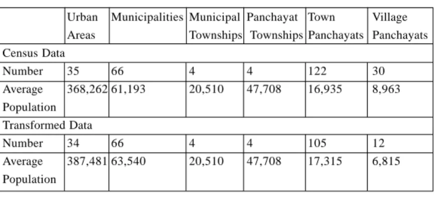
Table 2 : Status and Population of Towns in Tamil Nadu Urban Municipalities Municipal Panchayat Town Village Areas Townships Townships Panchayats Panchayats Census Data Number 35 66 4 4 122 30 Average 368,262 61,193 20,510 47,708 16,935 8,963 Population Transformed Data Number 34 66 4 4 105 12 Average 387,481 63,540 20,510 47,708 17,315 6,815 Population
14 For Berry, 20,000 inhabitants is the basic figure for defining a town (1971). Tiwari too points out the minor role of towns with less than 20,000 inhabitants in Tamil Nadu (Tiwari, 1996: 71 and later publications).
We note that in Table 2 some towns are classified as village panchayats. This apparent paradox is the result of the difference between the definition of a place as urban by the Census (or the regional administration) and the definition of its status defined according to the rules laid down by the Tax Department. If a place does not yield enough taxes to be classified as a town panchayat, but has all the Indian urban characteristics (more than 5,000 inhabitants, a density of more than 400 per square kilometre and more than 75 % of its active male population engaged in non-agricultural activities), it will be classified as a town while retaining its status of a village panchayat.
The small number of towns classified as villages and those classified as MTS and PTS, in terms of urban population (354,652 inhabitants in all or less than 2 % of the urban population), impelled us to withdraw them from most of the analyses (e.g. in Table 4, page 26) as the results obtained were not representative.
To understand fully how the urban system in Tamil Nadu is organised, we have classified towns according to their general economic specialisation. It must be remembered in fact that “the town’s specialised activity and the salaried jobs associated with it are good indicators of the dynamics of its economic and social base” (Pumain, Saint Julien, 1995: 48). Therefore, we decided to create a system for classifying the different types of towns in Tamil Nadu on the basis of their dominant economic activity.
To create this system of classification, we could have used a classification based on an ascending order, as is the common practice. This method, which is statistically effective, sometimes gives rise to groups whose boundaries are arbitrary and unintelligible. We therefore preferred to use a personal classification system that can be understood more easily. So, to determine the predominant activity, we chose a level corresponding to 50 % of the active population engaged in an
activity (a qualified majority). We were thus able to distinguish 7 kinds of towns on the basis of the dominant and secondary economic sectors, reflecting fairly accurately the geography of towns in Tamil Nadu.
Towns having a dominant agricultural sector: more than 50 % of the active population is engaged in an agriculture-related activity (including plantation workers and fishermen).
Towns having a dominant industrial sector: more than 50 % of the active population is engaged in an industrial activity or a craft. Towns having a dominant services sector: more than 50 % of the active population is engaged in services, trade, transportation, etc. Towns that are both agricultural and industrial: the proportion of active population engaged in each category is lower than 50 % and the total number of active persons in both the sectors taken together is higher than 70%.
Towns having dominant agricultural and services sectors: the proportion of active population engaged in each sector is lower than 50 % and the total number of active persons in both the sectors taken together is higher than 70 %.
Towns having dominant industrial and services sectors: the proportion of active population engaged in each sector is lower than 50 % and the total number of active persons engaged in both sectors taken together is higher than 70 %.
Mixed towns: towns that do not satisfy any of the preceding criteria and where the proportion of the active population engaged in each sector is lower than 40 %.
Table 3: Types of Towns in Tamil Nadu (absolute numbers and percentages)
Mixed Towns with Towns with Towns with Towns with Towns with Towns with Towns a dominant dominant dominant a dominant dominant a dominant
agricultural agricultural agricultural industrial Industrial services sector & services & industrial sector & services sector
sectors sectors sectors
8 (4 %) 31 (14 %) 48 (21 %) 9 (4 %) 22 (10 %) 28 (12 %) 79 (35 %)
It is not surprising that Table 3 reveals that the town is first and foremost a centre of services in Tamil Nadu because more than two-third towns specialise in the service sector. Specialisation in agriculture takes second place with 39% towns. Only 26% towns stand out because of the importance of industries.
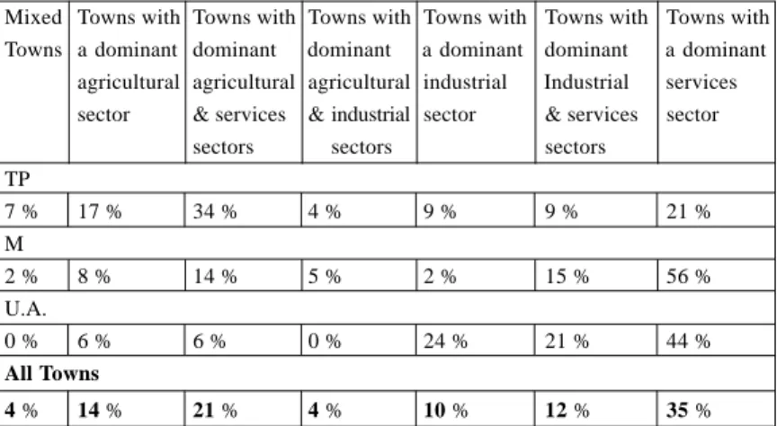
Table 4: Administrative Status and Urban Functions in Tamil Nadu
Mixed Towns with Towns with Towns with Towns with Towns with Towns with Towns a dominant dominant dominant a dominant dominant a dominant
agricultural agricultural agricultural industrial Industrial services sector & services & industrial sector & services sector
sectors sectors sectors TP 7 % 17 % 34 % 4 % 9 % 9 % 21 % M 2 % 8 % 14 % 5 % 2 % 15 % 56 % U.A. 0 % 6 % 6 % 0 % 24 % 21 % 44 % All Towns 4 % 14 % 21 % 4 % 10 % 12 % 35 %
Table 4 shows the relation between the status of a town and its predominant activity. Town Panchayats stand out due to the over-representation of agricultural activities, while municipalities concentrate on the services sector. Urban agglomerations have a mixture of services and industry. It is thus possible to arrange them
in a hierarchical order according to their respective roles: T.Ps are rural towns while municipalities act as administrative intermediaries and urban agglomerations are real full-fledged towns. It is nevertheless necessary to qualify this statement by recalling the spatial markers of economic specialisations, especially industrial activities, which form regional clusters (for detailed maps of Tamil Nadu, see Oliveau, 2003).
The major industrial zones in Tamil Nadu are well known. First, there is the Coimbatore plateau (stretching from Coimbatore to Salem), the Palar valley (with Vellore at its centre), the Sivakasi zone (to the south of Madurai and stretching to the west of Tirunelveli) and, to a lesser extent, the town of Neyveli to the south-west of Pondicherry. Similarly, the towns spawned by plantations in the Ghats dot the border with Kerala. There are many small predominantly agricultural towns all over the Cauvery delta. Besides, agriculture is often accompanied by the services sector giving these rural towns an intermediary role. Finally, all over the state there are towns dominated by the services sector, whose geographical distribution is generally correlated with population density.
3. From Towns to Rural Areas
Space has been integrated in economic thought from ancient times. It has always been difficult to accept it, especially because the integration of space in classical economic models ultimately raises more problems than it can solve (Derycke, 1994).
Nevertheless, the spatial dimension of uneven development has already been the subject of much thought. Thus the “core-periphery” model has been borrowed from economics (on this point, see Krugman, 2000), and subsequently reinterpreted in geographical space. Both geographers and economists study the notions of “core” and “centrality”. Conceptual exchanges between economic geography and spatial economics are common. Thus the spatial distribution of innovations, which is an old geographical
concept, has been borrowed to reinterpret the growth pole theory in spatial terms.
Sociologists too are concerned with the urban factor though their methods are different from those of geographers. The latter always play a role of prime importance, focusing on space even when social, economic or cultural issues are involved.
The town is a multidisciplinary object that has interested, among others, sociologists, economists and geographers who continue to study it intently. Geographers are quite logically interested in the spatial dimension of the change from urban to rural and several explanations can be suggested to understand the forms and reasons for this gradual shift.
a) Towns and rural areas: core and periphery?
In 1973, in his book Le développement inégal (Uneven Development), Samir Amin, concerned about the uneven economic development in the world, used the core-periphery binomial to describe the opposition between developed and developing countries. This association of terms was then considered in an economic context akin to Marxism where the core is the exploiter and the periphery is exploited. The spatial dimension is secondary and is used more in a metaphorical sense. But this idea leads to a more comprehensive view of the relations between societies (and spaces) that are dominant and dominated, giving rise to a shift from the social to the spatial dimension.
This pattern can be applied to different scales and this is one of its advantages. Thus, while it expresses the antagonism between developed and developing countries, it can also be adapted to understand the opposition (still considered in terms of domination) between the town (centre) and the rural areas (periphery). This dialectic opposition was taken up by geography because of its strong evocative power. Furthermore, its ability to describe the observed phenomena
in binary terms on any scale is very advantageous. Nonetheless, this approach is now obsolete. It is known that a part of the centre’s population (and even a part of its space) may be dominated and that the periphery need not consist only of social outcasts. In a wider context, the centre-periphery phenomenon may be treated as a peculiar and Manichean example of the concept of centrality. Centrality is a subjective perception of space. It can be used to define a point as being specific and different from the other points around it (Huriot, Perreur, 1994a). This point is then called the centre. It serves as a reference for structuring space. For example, this is how von Thünen creates his pattern: he starts with a village that he takes as the centre and looks at the spatial agricultural structure surrounding it according to its distance from this centre. So it is the central point that organises its surroundings in relation to itself. This pattern, originally envisaged for an “isolated state”, becomes more complex as the number of points increase. Let us not forget that centrality is neither absolute nor total. On the contrary, it is relative and contextualised: depending on the scale, it is relative to a given space; it is contextualised because the central point is defined by the nature of the study. In this context, Christaller’s theory of central places can be understood as a set of hierarchically arranged centres whose centrality is related to the level of observation (which defines the level of centrality) and dependent on the context (i.e. in its study of urban functions). To explain the creation of centres, one can refer to the economic theory of agglomeration economies. In brief, this theory considers an agglomeration as an economic element, having a relative advantage as compared to non-agglomerated zones15. In this
15 Krugman (2000: 50), said that we should not however leave ourselves open to jibes like the one made by the physicist who said, “So economists believe that companies agglomerate because of agglomeration economies”. Economic geography should therefore try to explain the forces of concentration in terms of more fundamental motivations.
way, an agglomeration, by differentiating itself from non-agglomerated zones, defines itself as a core. Further, this core then presents itself as a rival object competing with other objects, and this enables it to strengthen its position by becoming more attractive. This is what Huriot and Perreur call “the attractiveness of centrality” (Huriot, Perreur, 1994a: 50). This idea, which owes its origin to economics, can also be adapted to understand both social and cultural aspects.
Though the core attracts, it cannot however accommodate everything and this leads to the creation of a hierarchical order of objects at the core (Thisse, 2002), with the other objects organising themselves around this core, but not necessarily in a concentric manner because they can be influenced by other factors. The core then redistributes a part of the objects around it and thus increases its role in the geographical organisation of space. This redistribution can have two effects. We have a spill-over effect when the redistribution is positive and a backwash effect (Myrdal, 1957) when the concentration at the core brings about an economic deterioration at the periphery. It is this latter situation (where the most polluting enterprises start colonising the rural spaces to free the town, which is more of a rejection than a redistribution) that led Kundu to speak of “degenerated peripheries” (Kundu, 2003).
However, the core, apart from its function of attracting, can also act as a starting point. This is the “distribution centrality” defined by Huriot and Perreur (Ibid.). In fact, the core is also at the core of the spatial distribution of innovations (we are evidently referring to the work done by Hägerstrand, 1967). Therefore, when an innovation appears at a given point, this point distinguishes itself from the others and, according to the definition, constitutes a core. This core will then transmit the innovation (or information) to other points (the spill-over effect).
It is this perception of the distributive core that constitutes the basis of the growth pole theory. During the 1950s, F. Perroux explained that “growth does not appear everywhere at the same time; it is seen only at some points, or growth poles, and its intensity varies; it spreads through diverse channels and the end effects are different for the whole economy” (quoted by Manzagol, 1992: 496). One of the crucial ideas of the growth pole theory is that of propulsive industry: an enterprise introduces an innovation in a particular point of space and its development leads to the growth of the surrounding enterprises (through an increase in local consumption) and also of the enterprises it deals with (through an increase in the demand for production). This theoretical model was applied in the 1970s through the medium of various decentralisation policies, particularly in India.
One of the criticisms of this theory is that it depends on the point of view that is adopted. In fact, contrary to the idea that industrialisation encourages urbanisation by attracting people to industries, it is possible that populated areas give rise to new industries (Cassidy, 1997). This also explains the failure of the new industries set up in existing industrial zones (particularly in Africa), because the growth pole has not yet had a spill-over effect on the sparsely populated hinterland.
Nevertheless, all said and done, like Berry (1973), we feel that the growth pole theory is only one instance of the spread of innovation (Hägerstrand). That is why we are going to stress the influence of innovation on towns and rural areas.
b) Distance: “The first attribute of a spatial system”
One of the basic elements necessary to understand spatial distribution is distance. As a matter of fact, it defines the field of action of a transmission centre (the core) and makes it possible to measure the progression of innovations in space over a period of time.
1) Distance as a Connecting Factor
“Distance, the spatial dimension of separation, is a fundamental geographical property, influencing location and movement.” (Goodall, 1987: 134).
The word “distance” was borrowed (circa 1175) from a derivative of the Latin distantia, which actually means “stand apart” and also “difference” in the figurative sense. It is composed of the Latin prefix dis, which expresses the idea of separation, and the verb
stare meaning “to stand”. This led Roger Brunet (Brunet, Ferras,
Théry 1997) to remind us that Herodotus reported that the Persians had more respect for people who were closer to them. Though the writer may see in this a sign of ethnocentricity, we would prefer to point out that this semantic mixture of distance and difference, leads to the connection between near and similar that supports the idea of spatial auto-correlation.16
The present definition of the word still refers to this notion of separation but in a sense that is essentially spatial: « the length that separates one thing from another” (Rey-Debove, Rey 1996), in other words, an “interval between two points” (Brunet, Ferras, Théry 1997). Distance allows the measurement of the space separating two objects. However, while doing this, it creates a link between the objects17. Therefore, it is finally a connecting factor. It figures at the root of the geographical inquiry because “it is the only thing that can identify the location of a phenomenon in space and measure the difference in relation to the location in the geometric space of another phenomenon of the same type or even of a different type.”
16 “The literal meaning of spatial autocorrelation is self-correlation (autocorrelation)
attributable to the geographic ordering of data (spatial)” (Griffith, 1992: 2). In other
words, spatial autocorrelation is the dependence between the attributes of statistical individuals that are adjacent in space (Charre 1995).
17 For an anthropological opinion on the role of distance as a link between individuals, we will refer to Edward T. Hall’s classic work (1966).
(Chamussy, Chesnais, 1978:161). This is what makes distance “the first attribute of a spatial system” (Grataloup, 1996: 105).
If distance is the measurement of what separates or connects, the method of measurement can follow different paths, but we are only interested here in what is called “mathematical” distance (De Smith’s thesis, 2003, examines the question of distances). Mathematical distance is a special function that can be defined on the basis of the work done by Huriot and Perreur (1990: 200): “Any set of places; a real function d defined on L is a distance or
metric function, if and only if it satisfies the following 4
conditions, whatever a, b and c belonging to L may be (c1) non-negativity d
( )
a,b ≥0(c2) identity (c3) symmetry
(c4) triangular inequality d (a,b) ≤ d(a,c) + d(b,c)
The real number d(a, b) is called the distance from a to b.” The distance function is then defined by:
d p (A,B)= [(xAB)p
+ (yAB)p]1 / p , with x
AB = xA - xB ; yAB = yA - yB ; et p ≥ 1
The terms x
A and xB are the longitudes of points A and B (the
distance between which we wish to calculate), and yA and yB are their latitudes. The coefficient p is either higher than or equal to 1. For “p=1” we obtain a rectangular (or rectilinear) distance, which is also called “the Manhattan distance”. This distance is used to simulate urban movements because it is better suited than
( )
a,
b
0
a
b
d
=
⇔
=
( )
a,
b
d(b,
a)
the distance “as the crow flies” to assess the length18. The “distance as the crow flies” is a popular nomenclature of Euclidian distance. It is the most intuitive distance: the shortest route between two points. Its coefficient p is equal to 2.
When distance is expressed in this manner, it acquires two properties of mathematical models: it is ahistorical and spatially universal (Husain, 2001: 360). The ahistoricity of this factor is its unique value in time. If a point is at a distance of 10 km from another, that holds true for yesterday, today and tomorrow. Distance conceived in this manner is not dependent on time. This is also true of space: 10 km means the same thing whether one is in France, in the United States or in India. Distance is therefore a spatially universal factor.
These two elements are not inconsequential. Because of this ahistoricity and spatial universality it is in fact possible to make comparisons in time and in space. Mathematical distance does not have its own value, as it is objective. It can be easily expressed in the form of an equation and hence the use of mathematical tools for comparing, for example, the spatial distance of a town between one date and another or between different towns. The criterion for comparison is objective and it is mathematically formulated.
Nevertheless, this apparent objectivity should not conceal the problems raised by this approach. The first question is to find out what represents distance and if it can be used to explain social phenomena. Thus, although distance is an important explanatory factor for understanding the spatial structure of many phenomena, it remains just a structural characteristic of a situation.
18 This has been summarised very effectively by Pierre Dumolard (1999) in this pertinent question: “Has anyone ever seen birds flying straight from a starting point to the point of arrival?”
2) The Meaning of Distance in Tamil Nadu
Let us recall that “the intervention of distance lends itself to multiple interpretations” (Pumain, Saint Julien, 2001: 24). But we may agree that distance expresses first and foremost the “roughness of space” (Helle, 1993). Crossing distance, that is to say moving, implies a cost in terms of time in the first place: “distance is time” (Grataloup, 1996: 86); and also in financial terms. We find that the distance-time and distance-cost mentioned above are actually distortions of mathematical distance. In other words, “they are the weighting of raw distance according to criteria which are exogenous to space in order to express the interaction between theoretical aspects and physical constraints” (Lemay, 1978: 151). Though these distances often improve the understanding of phenomena, they are much more difficult to include in a model.
The friction of distance (imposed by the “roughness of space”) constitutes a constraint on human movement. In societies where the level of technology is low, this friction is very strong, which leads Paul Bairoch to speak of the “tyranny of distance” (Bairoch, 1985: 33). Because, though distance is universal as far as its measurement is concerned, crossing it is extremely contextual. Movement depends both on the nature of the terrain to be crossed and on the technical means available.
Therefore, in Tamil Nadu in 1991, we were able to distinguish three main forms of movement: walking, riding and public transport. Each of these means has its own speed, which can be estimated at about 5 km/h for walking, about 10 km/h for a bicycle and 30 to 40 km/h for a bus. This range of speeds is important to understand periurbanisation.
If one considers that an individual is not usually prepared to spend more than one hour to reach his or her place of work, it is possible to prepare a model of the average interaction with the nearest town
in the following manner: the poorest individuals living more than 5 km away visit the town very rarely. Individuals possessing a bicycle will be limited by a distance of about ten kilometres. As for public transport, only some individuals can afford it, but not for a distance of more than 30 to 40 km.
c) Choosing one’s distance
For our study, we had to define the metric function and the specific distance we used. We opted for Euclidian distance because it provides the best information suited to the scale of our study, rectilinear distances being more suited to intra-urban studies and spherical distances to calculations on a smaller scale. Peeters and Thomas have shown that in the absence of a major obstacle, i.e. in Euclidian spaces, Euclidian distance is a good approximation. They also remind us that the use of a non-Euclidian distance means working in non-Euclidian spaces (Peeters and Thomas, 1997: 66). We chose to measure the distance keeping in mind the town’s administrative boundary as defined by the census and not in relation to its centre.
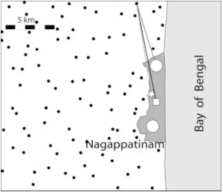
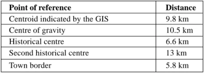
Measurement in relation to the centre posed two major problems. The first was related to the definition of the centre in a country where towns are often polycentric. The second problem was related to the result we wished to obtain. We wanted to know the impact of the town and not the influence of the distance to the centre. We have therefore looked at towns as homogenous entities, which begin to influence rural spaces from their border and not from their centre. We therefore opted for a calculation based on the administrative border as defined by the census. Though this border, like all information provided by census maps, is suspect, it is not more so than the centre, which has been determined on the same basis. Comparisons between census maps and other maps of the cities of Chennai and Pondicherry however proved to be quite satisfactory. Further, this measurement takes into account the shape of the towns and improves the calculation of the distance (see diagram). All the
results that are presented are therefore the distances of villages to the border of the nearest town. It may also be noted that during calculation, the identity of the nearest town is given, which makes it possible to assign villages to towns. This will be very useful for differentiating the urban impact according to the characteristics of the towns.
Figure 2 : Should the measurement be taken from the centre or from the town’s border ?
Figure 2 shows the difficulties quite clearly and the implications of the initial choice for calculating the distance of villages (black dots) to the nearest town (Nagappatinam, in dark grey for this example). The centroïd indicated by the GIS19 (White Square with