Publisher’s version / Version de l'éditeur:
Cement and Concrete Research, 36, July 7, pp. 1312-1323, 2006-07-01
READ THESE TERMS AND CONDITIONS CAREFULLY BEFORE USING THIS WEBSITE.
https://nrc-publications.canada.ca/eng/copyright
Vous avez des questions? Nous pouvons vous aider. Pour communiquer directement avec un auteur, consultez la
première page de la revue dans laquelle son article a été publié afin de trouver ses coordonnées. Si vous n’arrivez pas à les repérer, communiquez avec nous à PublicationsArchive-ArchivesPublications@nrc-cnrc.gc.ca.
Questions? Contact the NRC Publications Archive team at
PublicationsArchive-ArchivesPublications@nrc-cnrc.gc.ca. If you wish to email the authors directly, please see the first page of the publication for their contact information.
NRC Publications Archive
Archives des publications du CNRC
This publication could be one of several versions: author’s original, accepted manuscript or the publisher’s version. / La version de cette publication peut être l’une des suivantes : la version prépublication de l’auteur, la version acceptée du manuscrit ou la version de l’éditeur.
For the publisher’s version, please access the DOI link below./ Pour consulter la version de l’éditeur, utilisez le lien DOI ci-dessous.
https://doi.org/10.1016/j.cemconres.2006.01.015
Access and use of this website and the material on it are subject to the Terms and Conditions set forth at
Sensitivity analysis of simplified diffusion-based corrosion initiation
model of concrete structures exposed to chlorides
Zhang, J. Y.; Lounis, Z.
https://publications-cnrc.canada.ca/fra/droits
L’accès à ce site Web et l’utilisation de son contenu sont assujettis aux conditions présentées dans le site LISEZ CES CONDITIONS ATTENTIVEMENT AVANT D’UTILISER CE SITE WEB.
NRC Publications Record / Notice d'Archives des publications de CNRC: https://nrc-publications.canada.ca/eng/view/object/?id=5459ffe7-0f36-4937-a135-821b73cf81fc https://publications-cnrc.canada.ca/fra/voir/objet/?id=5459ffe7-0f36-4937-a135-821b73cf81fc
http://irc.nrc-cnrc.gc.ca
Sensitivity analysis of simplified diffusion-based corrosion
initiation model of concrete structures exposed to chlorides
N R C C - 4 8 3 7 3
Z h a n g , J . ; L o u n i s , Z .
A version of this paper is published in / Une version de ce document
se trouve dans: Cement and Concrete Research, v. 36, no. 7, July
Sensitivity Analysis of Simplified Diffusion-Based Corrosion Initiation Model
of Concrete Structures Exposed to Chlorides
Jieying Zhang∗ and Zoubir Lounis
National Research Council Canada Institute for Research in Construction
Ottawa, ON, K1A 0R6, Canada
ABSTRACT
This paper presents the results of a sensitivity analysis of the diffusion-based corrosion initiation model
for reinforced concrete structures built in chloride-laden environments. Analytical differentiation
techniques are used to determine the sensitivity of the time to corrosion initiation to the four governing
parameters of the model, which include chloride diffusivity in concrete, chloride threshold level of steel
reinforcement, concrete cover depth, and surface chloride concentration. For conventional carbon steel,
the time to corrosion initiation is found to be most sensitive to concrete cover depth, followed by chloride
diffusion coefficient, with normalized sensitivity coefficients of about 2 and −1. For corrosion-resistant steels, the time to corrosion initiation is most sensitive to the surface chloride concentration and chloride
threshold level followed by the concrete cover depth and chloride diffusion coefficient. The results of this
sensitivity analysis are discussed in detail, including the variations in predicted time to corrosion initiation
induced by variations of the four model parameters and their implications for design and maintenance of
concrete structures built in corrosive environments.
Keywords: chloride diffusion (C), corrosion initiation (C), sensitivity analysis.
∗
INTRODUCTION
Chloride-induced corrosion of the steel reinforcement is identified as the main cause of deterioration of
different types of concrete structures (e.g. bridges, parking garages, off-shore platforms, etc.). The sources
of chlorides are the seawater and deicing salts used during winter. The corrosion of the steel
reinforcement leads to concrete fracture through cracking, delamination and spalling of the concrete
cover, reduction of concrete and reinforcement cross sections, loss of bond between the reinforcement and
concrete, and reduction in strength and ductility. As a result, the safety and serviceability of concrete
structures are reduced. One of the earliest studies on corrosion of reinforcing steel embedded in concrete
structures was reported by Stratfull (1956), in which chlorides and moisture were identified as the main
causes for extensive corrosion in reinforced concrete bridge piers built in a marine environment after only
seven years from initial construction. In the last three decades, chloride-induced corrosion of reinforced
concrete structures has been extensively studied (Gouda 1970; Tuutti 1982; Rosenberg et al. 1989; Cady
and Weyers 1983), particularly, as a result of the high costs of highway bridge repair in North America
and Europe from the effects of de-icing salts used during winter or from seawater for costal structures.
A reliable prediction of the time to corrosion initiation of concrete structures exposed to chlorides is
critical for the selection of a durable and cost-efficient design and for the optimization of the inspection
and maintenance of built structures, which is essential to minimize the life cycle costs. Existing models
are mostly based on the assumption of a Fickian process of diffusion for predicting the time and space
variations of chloride content in concrete and on the concept of chloride threshold to define the corrosion
resistance of reinforcing steel to chloride attack. Therefore, the governing parameters of this
diffusion-based corrosion initiation time include the concrete cover depth, chloride diffusion coefficient in concrete,
surface chloride concentration, and chloride threshold level assuming the presence of moisture and
oxygen for the corrosion to proceed. In practice, the design of durable concrete structures is mainly based
water-to-cement ratio (to achieve low chloride diffusivity), and as well the use of more corrosion resistant
reinforcing steels (e.g. stainless steel).
However, a considerable level of uncertainty may be associated with one or more of the above identified
parameters. This is due to: (i) heterogeneity and aging of concrete with temporal and spatial variability of
its chloride diffusivity; (ii) variability of concrete cover depth, which depends on quality control,
workmanship and size of structure; (iii) variability of surface chloride concentration, which depends on
the severity of the environmental exposure; and (iv) uncertainty in chloride threshold level that depends
on the type of reinforcing steel, type of cementing materials, test methods, etc. (Bamforth and Price
1997). It is clear that the combination of these uncertainties leads to a considerable uncertainty in the
model output, i.e. the time to corrosion initiation. This uncertainty in the model output could have serious
consequences in terms of reduced service life, inadequate planning of inspection and maintenance and
increased life cycle costs.
Therefore, undertaking a sensitivity analysis becomes imperative to assess the impact of uncertainties
from the input parameters on the uncertainty of the model output. In the literature, several methods and
techniques have been used for the sensitivity analysis of different types of models in different fields of
applications, including Monte Carlo simulations, response surface methods, differential analysis
techniques, nominal range sensitivity analysis, etc. (Saltelli et al. 2000). Fewer sensitivity studies are
found in the literature that deal with the performance of concrete structures that incorporate or evaluate
the impact of the uncertainties in the model parameters on the model output, such as service life (Boddy
et al. 1999; Lounis et al. 1998, 2000, 2004; Melchers 1987).
In this paper, a sensitivity analysis of the diffusion-based model for time to corrosion initiation using the
differential analysis technique is undertaken to identify the most significant parameters and quantify their
corrosion initiation caused by variations in the input data of the model, which include concrete cover
depth, chloride diffusion coefficient, surface chloride concentration, and chloride threshold level. The
results of a sensitivity analysis can provide valuable insights and a better understanding of the chloride
diffusion-induced corrosion of reinforcing steel in concrete and its governing parameters. Sensitivity
analysis can be used to identify the importance of uncertainties in the model input for the purpose of
prioritizing additional data collection or research on the parameters that are found significant.
Furthermore, the results of a sensitivity analysis can provide effective decision support in the design of
durable new structures, as well as in the optimization of inspection and maintenance of existing
structures.
DIFFUSION-BASED CORROSION INITIATION MODEL
2.1 Chloride Ingress Into Concrete Structures
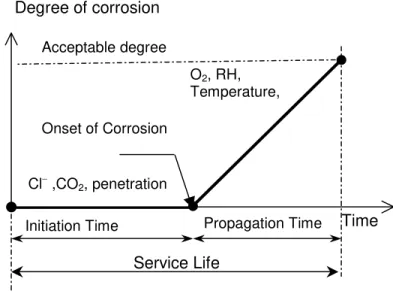
The corrosion of concrete structures can be described as a two-stage process: (i) corrosion initiation stage;
and (ii) corrosion propagation stage (Tuutti 1982) as illustrated in Figure 1. For chloride-induced
corrosion, the initiation stage corresponds to the period of time during which chlorides penetrate the
concrete but no damage is observed. The corrosion initiation time is defined as the time at which the
concentration of chlorides at the steel surface reaches a critical or threshold value. The propagation stage
corresponds to the period of time during which corrosion products accumulate and initiate fracture of
concrete and ultimately failure. The service life of concrete structures in chloride-laden environments can
be defined as the sum of the durations of the two stages. In general, the durability and serviceability of
concrete structures depend greatly on the duration of the initiation stage. As a result, a reliable prediction
model of chloride penetration into a reinforced concrete structure is of utmost importance in predicting
the time to corrosion initiation, as well as the total service life.
Aggressive agents such as chlorides, water, and oxygen penetrate into concrete through the pore spaces in
concrete and more particularly on the water-cement ratio of the concrete mix and the presence of
supplementary cementing materials (e.g. silica fume, fly ash, or slag) and/or protective systems that delay
or slow down chloride ingress. In porous solids, such as concrete, moisture may flow via the diffusion of
water vapor, and via non-saturated or even saturated capillary flow in finer pores (Kropp and Hilsdorf
1995). Chloride ingress into concrete from external sources is therefore due to multiple transport
mechanisms, such as diffusion and adsorption. However, adsorption occurs in concrete surface layers that
are subjected to wetting and drying cycles, and it only affects the exposed concrete surface down to 10-20
mm (Weyers et al. 1993; Tuutti 1996). Beyond this adsorption zone, the diffusion process will dominate
(Tuutti 1996).
Chloride diffusion is a transfer of mass by random motion of free chloride ions in the pore solution
resulting in a net flow from regions of higher to regions of lower concentration (Crank 1975). The rate of
chloride ingress is proportional to the concentration gradient and the diffusion coefficient of the concrete
(Fick’s first law of diffusion). Since in the field, chloride ingress occurs under transient conditions, Fick’s
second law of diffusion can be used to predict the time variation of chloride concentration for
one-dimensional flow, as follows:
] [ ) , ( x C D x t t x C ∂ ∂ ∂ ∂ = ∂ ∂ (1)
Under the assumptions of a constant diffusion coefficient, constant surface chloride content Cs as the
boundary condition, and the initial condition specified as C=0 for x>0, t=0, Crank’s solution of Eq. (1)
yields (Crank 1975): )] Dt x erf( [ C dη e π C C(x,t) Dt s x η s 2 1 2 1 2 0 2 − = ⎥ ⎦ ⎤ ⎢ ⎣ ⎡ − =
∫
− (2)where: C(x,t) is the chloride concentration at depth x after time t; Cs is the chloride concentration at the
2.2 Corrosion of Reinforcing Steel
As seen in Tuutti’s corrosion model in Figure 1, the corrosion initiation stage corresponds to the process
of chloride transport onto a steel surface, while the steel remains passivated with a corrosion rate lower
than a defined level, e.g. 0.1 μA/cm2 (González et al. 1980). The onset of corrosion of the reinforcing
steel is assumed to start when the concentration of chlorides at the level of the reinforcement has reached
the so-called “chloride threshold level” Cth, which destroys the passivation of steel. Therefore, the
duration of the initiation stage is from time zero to the onset of corrosion. The initiation stage and onset of
corrosion in Tuutti’s model can be stated mathematically as follows:
Initiation stage: C(dc,t) < Cth for 0≤ t < Ti (3a) Onset of corrosion: C(dc,t) = Cth for t= Ti (3b)
where Ti is the time to onset of corrosion (equivalent to time to corrosion initiation) and dc is the depth of concrete cover over the reinforcing steel. Substituting the condition of onset of corrosion in Eq. (3b) into Eq. 2, and assuming the same initial and boundary conditions, the time to corrosion initiation is determined as follows: 2 1 2
)]
1
(
[
4
)
,
,
,
(
s th c c th s iC
C
erf
D
d
d
D
C
C
f
T
−
=
=
− (4)The above equation represents a transformation of Crank’s solution of chloride concentration in concrete
into a deterministic model of the time to corrosion initiation as an explicit function of the parameters, Cs,
Cth, D, and dc. These governing parameters can be categorized as follows: (i) structural parameter:
concrete cover depth; (ii) material parameters: type of concrete and corresponding chloride diffusivity
(D), which is an indicator of the accessibility of concrete to chloride penetration; and type of reinforcing
steel and corresponding chloride threshold level (Cth), which is a measure of its corrosion resistance; and
(iii) environmental parameter (Cs), which is a measure of the corrosion load or risk on the structure.
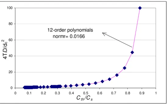
Given the complexity of the error function and its inverse, a 12th order polynomial was found to be a best
m s th m m c c th s i
C
C
A
D
d
d
D
C
C
f
T
[
]
4
)
,
,
,
(
12 0 2∑
==
=
(5)where the coefficients A0 to A12 of the polynomial are listed in Table A in Appendix. A plot of 2
4
c id
DT
versus s thC
C
is shown in Figure 2SENSITIVITY ANALYSIS USING DIFFERENTIATION TECHNIQUE
3.1 Uncertainty in Corrosion Initiation Time
Despite the simplicity and extensive use of the above diffusion-based corrosion initiation model,
considerable uncertainties are associated with its governing parameters and predictions. There are various
sources of uncertainty, which include physical uncertainty, statistical uncertainty, and model uncertainty.
The physical or inherent uncertainty is that identified with the inherent random nature of the main
parameters of the model (e.g. uncertainties in concrete cover depth, surface chloride concentration,
chloride diffusion coefficient, and chloride threshold level). The statistical uncertainty arises from
estimating the mean value and possibly the standard deviation of each of the governing parameters from a
limited sample size. The model uncertainty arises from the use of simplified mathematical models or
relationships between the basic variables to represent the actual physical phenomena of chloride ingress
and corrosion initiation. The main factors that contribute to the uncertainty of the diffusion-based model
can be summarized as follows:
1. Assumptions of chloride transport mechanism governed by diffusion and one-dimensional flow
solution from the surface into a half space;
2. Use of the simplified concept of chloride threshold level to define the corrosion resistance of
reinforcing steel embedded in concrete structures. A considerable scatter of this threshold value is found
3. Assumption of time-invariance and independence of concrete parameters:
A. The diffusion coefficient is not a constant but rather depends on time, temperature, and depth
because of the heterogeneous nature and aging of concrete, as mentioned earlier. For many concrete
structures (e.g. bridge decks), the top surface is subjected to a continually changing chloride exposure. As
a result, the chloride concentration at the surface varies with time; however at some shallow depth, it can
be assumed as a quasi-constant (Weyers et al. 1993; Kropp and Hilsdorf 1995).
A. The concrete cover depth is variable and the level of variability depends on the quality of
construction and size of the structure.
C. The coefficients of variation of the governing parameters are quite high and may vary between
10% to 40% and for some, up to 80% (Cady and Weyers 1983; Lounis 2004).
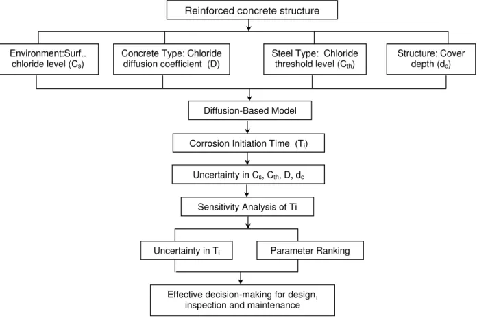
Figure 3 illustrates the proposed procedure for the incorporation of parameter uncertainty in model
prediction of time to corrosion initiation in this paper. The previous sections have discussed 1) the
diffusion based model with the four governing parameters; and 2) the time to corrosion initiation is
established based on the diffusion model and Tuutti’s corrosion model. In summary, this section has
concentrated on the uncertainties in the four parameters to be used in the sensitivity analysis in the next
section.
3.2 Need for Sensitivity Analysis
It is clear from the above that a significant uncertainty or error can be associated with the prediction of the
time to corrosion initiation (Ti) by using the above simplified diffusion model. The following questions
then arise:
1. How to assess the errors in predicting the time to corrosion initiation by using the simplified diffusion
model?
2. Which parameters have the greatest impact on Ti ?
4. How to use these results for engineering purposes, to achieve effective design, inspection, and
maintenance of concrete structures.
The first question can be answered by undertaking an analysis of the sensitivity of Ti to the four
governing parameters. One result of the sensitivity analysis (see Figure 3) is to provide the levels of
variation (or uncertainty) in Ti that are induced by variations in each of the four parameters over a feasible
range of variation, which must be quantified and understood before this model is used in service life
predictions. For instance, the time to corrosion initiation varies over a wide range (e.g., the variation is
from 10 years to 50 years for a design value Ti of 30 years) due to a realistic variation of the parameters
(e.g., actual concrete cover is found to vary from 10 mm to 50 mm, when the design value was 30 mm). It
is therefore clear that the use of the above deterministic model has serious shortcomings.
Another result of the sensitivity analysis (see Figure 3) is to provide a ranking of parameter importance,
which can then be used to answer the questions raised above. By identifying the most relevant parameters
affecting the time to corrosion initiation (Ti), it is possible to provide the decision maker with very
relevant information regarding which parameters to control to achieve a given design service life, or Ti,
and how to implement measures (quality control, inspection, maintenance) in order to reduce the
uncertainties with those critical parameters in order to reduce the uncertainty in Ti.
Therefore, when this diffusion-based model is used to study the sensitivities of Ti to variations in its
governing parameters, the variations are no longer noise but are used to quantify their impact on Ti. The
results of the sensitivity study will therefore help in effective decision-making for design, inspection, and
maintenance (see Figure 3). Several methods have been developed and applied for sensitivity and
uncertainty analysis, including:(i) nominal range sensitivity analysis; (ii) difference in log-odds ratio; (iii)
sensitivity test; (vii) Bayesian sensitivity analysis, etc. (Saltelli et al. 2000; Melchers 1987). These
methods vary in level of complexity, data requirements, representation of the sensitivity and specific uses.
In this paper, the differential analysis method is used to investigate the sensitivity of the diffusion-based
time to corrosion initiation model to the four basic parameters of concrete structures exposed to chlorides.
This method is easy to apply and provides relevant information on the impact of the different parameters
on the model output and ranking of their relative importance. It requires a limited amount of data related
to the governing parameters, namely their mean or base values and possibly their standard deviations,
which is not the case for Monte Carlo simulation, which requires complete probabilistic distributions of
all parameters. The description of the technique is given in the next section.
3.3 Sensitivity of Corrosion Initiation Time Using Differentiation Analysis
Differential sensitivity analysis is based on using a Taylor series to approximate the model under
consideration. This approximate model is used as a surrogate for the original model in the sensitivity
analysis. The diffusion-based corrosion initiation time model of Eq. (4) can be represented as the
following function:
Ti =f(Cs, Cth,D,dc)= f(X1,X2,X3,X4) (6)
Where the governing parameters are the input variables and are represented by the vector:
X=[X1,X2,X3,X4] (7)
A first-order Taylor series approximation of Ti has the following form, with X0 represents a base value
vector (or reference vector):
)
(
)
(
)
(
)
(
4 1 0 0 j jo j j i iX
X
X
X
f
X
T
X
T
−
∂
∂
+
≅
∑
= (8)The values of the partial derivatives are a measure of the local sensitivity. Higher order expressions can
also be derived. The order of the approximation depends on the curvature of the surface of Ti =f(X).
jo jo j i jo j j i i i
X
X
X
X
T
X
X
X
f
X
T
X
T
X
T
(
)
)
(
)
(
)
(
)
(
)
(
0 4 1 0 0 0−
∂
∂
=
−
∑
= (9) LetΔ
T
i=
T
i(
X
)
−
T
i(
X
0)
(10a) (10b) jo j jX
X
X
=
−
Δ
andT
i(
X
0)
=
T
i0 (10c)In this approach, inference about the variability of Ti or f(X) is made by changing one parameter or one
factor at a time and keeping the other parameters constant (equal to their base-values) and investigating
the change in Ti, therefore:
0
=
∂
∂
kx
f
k=1,2,…, n with k≠j (11a) and '( j) j x f xf = ∂ ∂ (11b)Therefore, Eq. (9) becomes:
j j i jo j io jo i
S
X
S
T
X
X
X
f
T
X
X
T
=
=
∂
∂
=
Δ
Δ
)
(
)
(
0 0 (12a)where Sj is the normalized first-order sensitivity coefficient of Ti to Xj, which provides a measure of the
relative change in Ti that results from a relative change in Xj , when the other variables are kept constant.
It should be noted that the change or perturbation in Xj should be small, i.e. a small fraction of its base (or
mean) value. 0 0
)
(
i jo j jT
X
X
X
f
S
∂
∂
=
j=1,..,4 (12b) Given the assumption of one variable parameter at a time, it is possible to include the higher order termsof the Taylor series approximation to determine the higher order sensitivity coefficients Sh(Xj) by using
1 1 ) ( )! 1 ( ) ( ) ( ! ) ( ... ) ( ' ) ( ) ( + + Δ + + Δ + + Δ = − Δ + = Δ n j j n n j j n j j j j i X n X f X n X f X X f Xj f X X f T
θ
(13)where fn denoted the nth order derivative of f(Xj) for
X
j<
θ
X
j<
X
j+
Δ
X
j. Substituting Eq. (13) into Eq. (12b) yields: ] ) ( )! 1 ( ) ( ) ( ! ) ( ... ) ( ' [ ) ( 1 1 0 0 0 n j j n n j j n j io j j h hj X n X f X n X f X f T X X S S Δ + + Δ + + ∗ = = + − θ (14)Since Sj (or Shj) is a dimensionless quantity, the sensitivities to the independent variables with different
dimensions could be compared. From the values of coefficients Sj, the following conclusions can be
made:
1. The sign of the coefficient Sj indicates whether Xj and Ti tend to move up or down together or in
opposite directions. A positive value of Sj means that a change in Xj will result in a change in Ti in the
same direction, and visa versa.
2. The absolute values of these coefficients can be used to rank the relative importance of the individual
parameters. It can be concluded that Ti is more sensitive to the variable Xm rather than Xn if the absolute
value of S(Xm) is greater that of S(Xn), denoted by ⏐S(Xm)⏐> ⏐S(Xn)⏐.
Using Eq.(12b), the first-order sensitivity coefficients of Ti to Cs, Cth, D, or dc, can be obtained as follows:
2
)
(
'
)
(
=
=
i c c cT
d
d
f
d
S
(15)(
)
=
'
(
)
=
−
1
iT
D
D
f
D
S
(16) Let(
,
)
1(
1
)
s th th sC
C
erf
C
C
g
=
−−
(17) Then 2 )] , ( [ 1)
1
(
)
(
'
)
(
th sC C g s th s th i s s se
C
C
erf
C
C
T
C
C
f
C
S
− −−
−
=
=
π
(18)and 2 )] , ( [ 1
)
1
(
)
(
'
)
(
th sC C g s th s th i th th the
C
C
erf
C
C
T
C
C
f
C
S
− −−
=
=
π
(19)The first order sensitivity coefficients of Ti to dc and D are easily computed and are found to be constant.
The first order sensitivity coefficients of Ti to Cs or Cth, however, are complex functions of the variables
Cs and Cth, so are the higher order sensitivity coefficients. It is therefore impractical to use Eq. (14) to
calculate ΔTi from ΔCs or ΔCth. As noted before, 2
4
c id
DT
versus s thC
C
is equivalent to ξ versus γ, where
2
1
x
=
ξ
,γ = 1-y, and y=erf(x), and the numerical relationship between ξ and γ is obtainable (e.g. Figure 2) given the numerical relationship between x and y. As a result, ΔTi / Ti versus ΔCth /Cth can be derived from the above as equivalent to Δξ/ξ versus Δ γ/γ, considering that the other variables are kept constant. The numerical correlation between Δξ/ξ and Δ γ/γ is obtained if the base values of ξ and γ isSpecified. Similarly, the numerical correlation between ΔTi /Ti and ΔCs /Cs can be obtained using the same approach. A more practical approach is to plot first the variations of ΔTi/Ti versus ΔCs/Cs (or ΔCth /Cth) and then a regression analysis can be carried out to obtain the analytical correlation that yields satisfactory precision.The higher order derivatives of Ti to D or dc are easily obtained, from which high-order sensitivity
coefficients Sh(D) and Sh(dc) of Ti to D and dc can be obtained as follows:
1 + Δ Δ − = Δ D D D D T T i i (20a) 1 1 ) ( S + Δ − = D D D h (20b)
)
(
2
2 c c c c i id
d
d
d
T
T
Δ
+
Δ
=
Δ
(21a)c c c h
d
d
d
S
(
)
= 2
+
Δ
(21b)It should be noted that the four variables Cs, Cth, D, and dc are assumed to be independent variables in
this paper in order to illustrate the dependence of Ti on each of them. In reality, D and Cth may be
correlated because both are related to concrete properties. The chloride diffusion coefficient is a material
property of concrete dependent primarily on its pore structure and saturation of the pore solution; the
parameter Cth of the reinforcing steel depends also on the concrete chemistry, mainly the pH level of the
concrete pore solution. However, Cth is treated here as an independent steel property because other
parameters are kept constant when the sensitivity to Cth is analysed.
4. RESULTS OF SENSITIVITY ANALYSIS
4.1 Ranges of Variation of Governing Parameters
Realistic ranges of variation of the four governing parameters used in this study, Cs, Cth, D, and dc, are
summarized below from a literature review, with emphasis on bridge deck applications.
4.1.1 Surface chloride concentration
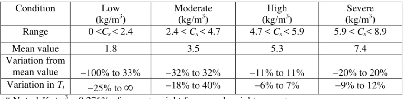
Weyers et al. (1993) classified the corrosive environments surrounding bridge decks into four categorizes
in terms of surface chloride concentration Cs: light, moderate, high, and severe exposures. As shown in
Table 1, the mean values, Cs, of the four exposures are 1.8 kg/m3, 3.5 kg/ m3, 5.3 kg/ m3,and 7.4 kg/ m3,
respectively; and the variations in these categories from the mean values, ΔCs /Cs, are from −100% to +33%, ±32%, ±11%, and ±20%, respectively. For example, a concrete structure exposed to a moderate environment can be estimated to have a Cs=3.5 kg/m3, if an accurate value is not available (which is often
the case); this estimated mean value is associated with a variation of ±32%.
4.1.2 Chloride threshold level
of the steel in concrete will be destroyed. It depends on the type of steel, electrochemical environment in
concrete, and testing method (Bamforth and Price 1997; Alonso et al. 2000) and consequently, a
considerable variation is expected for this parameters. Different types of steel have different Cth, and even
one type of steel (e.g. carbon steel) has a wide range of reported Cth.
In this regard, values from one research investigation are considered for this study in order to minimize
the variation induced by the testing methods. Trejo and Pillai (2003 and 2004) reported that the mean
values of Cth for carbon steel (ASTM A615), micro-composite steel, stainless steel SS304 and SS316LN,
are 0.52 kg/m3, 4.6 kg/m3, 5.0 kg/m3, and 10.8 kg/m3, respectively, as summarized in Table 2. Since the
experimental designs and test procedures were the same for these different steels, their reported variations
from the mean values can be considered as the “intrinsic” variations of the steels, which are ±40%, ±16%, ±19%, and ±12%, respectively, as seen in Table 2.
4.1.3 Chloride diffusion coefficient
The chloride diffusion coefficient D of concrete is a material property that is a measure of the rate of
chloride penetration into concrete. The value of D depends on both concrete mix design, such as
water/cement ratio, quantity of mineral admixtures, aggregation fraction, etc., and other parameters such
as temperature and age of concrete (Bentz 2000; Thomas and Bamforth 1999). The typical values of D for
normal Portland cement concrete (e.g. w/c=0.4) were reported between 10−12 m2/s and 10−11 m2/s (Bijen
1996; Thomas and Bamforth 1999), e.g. D= 4×10⁻¹²
m2/s for a normal concrete with w/c=0.4 and D=
10−11 m2/s for w/c=0.55 (Bijen 1996). The incorporation of mineral admixtures (e.g. fly ash, slag, silica
fume), however, can lead to orders of magnitude reduction of D in the long term (Thomas and Bamforth
1999). In this study, D is considered to vary from 10−12 m2/s to 10−11 m2/s.
The concrete cover depth dc is a design parameter that varies with the severity of the environmental
exposure and depends on the quality of workmanship and control during construction. For cast-in-place
bridge decks, its value could vary from 20 mm to 80 mm for average to below average quality control
(Lounis 2004).
4.2 Ranking of Parameter Importance
As expected, it can be seen from Eqs. (15) to (19) that the sensitivity coefficients of the time to corrosion
initiation Ti to concrete cover, S(dc), and to chloride threshold level, S(Cth) are positive, which means that
increasing dc or/and Cth will increase Ti. On the other hand, the sensitivity coefficients of the time to
corrosion initiation Ti to surface chloride concentration, S(Cs), and to chloride diffusion coefficient, S(D)
are negative, which means that increasing Cs or/and D will decrease Ti.
The values of S(dc) and S(D), are constant and equal to 2 and –1, respectively, which indicate that Ti is
much more sensitive to dc than D. On the other hand, the values of S(Cth) and S(Cs) are both functions of
the Cth/Cs ratio, which depends primarily on the corrosion resistance of the reinforcing steel and
environmental exposure. Figure 4 represents plots of the variations of the sensitivity coefficients of Ti to
the four governing variables versus the Cs/Cth ratio, which is varied from 1 to 10, representing an
increasingly corrosive environment for a given steel reinforcement. Figure 4 shows that both
⏐S(Cth)⏐and⏐S(Cs)⏐decrease exponentially with increasing Cs/Cth ratios from values higher than 4 and decrease asymptotically towards zero.
4.2.1 Case of conventional black carbon steel
From Table 1 and Table 2, Cs/Cth ratios for conventional black carbon steel may vary from 3.5 to 14.2
depending on the environmental exposures. In this range, as shown in Figure 4, the time to corrosion
initiation is most sensitive to concrete cover, then to chloride diffusion coefficient, and least to surface
means that increasing concrete cover depth for carbon steel reinforcement is the most effective measure to
increase the service life, followed by increasing the quality of concrete.
|S(dc) | > |S (D) |> |S (Cth) |=|S(Cs) | (22)
4.2.2 Case of corrosion resistant steels
From Table 1 and Table 2, Cs/ Cth ratios for corrosion resistant steels could be less than 1.6. In this range,
as shown in Figure 4, the time to corrosion initiation is most sensitive to surface chloride concentration or
chloride threshold, then concrete cover, and least to chloride diffusion coefficient, which yields the
ranking shown in Eq.(23). It implies that for concrete structures using high corrosion resistant steels, it is
critical to use a precise value of chloride threshold in order to properly assess the service life.
|S (Cth) |= |S(Cs) | > |S(dc) | > |S(D) | (23)
4.3 Sensitivity of Time to Corrosion Initiation to Diffusion Model Parameters
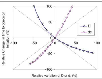
4.3.1 Sensitivity to chloride diffusion coefficient
Equation (20a) evaluates the effect of a relative change in D, (denoted by ΔD/D), on Ti, and the impact of ΔTi/Ti of ΔD/D is plotted in Figure 5, from which the following two main observations can be made: 1. For variations in D of less than 10%, Sh(D) is approximately equal to −1, which is the first-order sensitivity e.g., a 10% increase in D will decrease Ti by about 9%.
2. The increase and decrease in Ti are asymmetrical with D; a much greater change in Ti will be made by a
decrease in D than an increase in D for the same percentage. For example, a 50% reduction in D,
increases Ti by 100%, while a 50% increase in D will reduce Ti by about 33 %.
Therefore, a precise assessment of D should be sought in practice, since variations of D of ±50%, (which are small variations in practice as noted earlier), could lead to variations in Ti ranging from –33.3% to
+100%. It also implies that a small decrease in chloride diffusion coefficient would greatly extend the
unknown D, it is more appropriate to estimate it in a conservative manner, to avoid an overestimation of
the service life. The practical effect of D is further illustrated by the following study in which D is varied
from 10−12 m2/s to 10−11 m2/s.
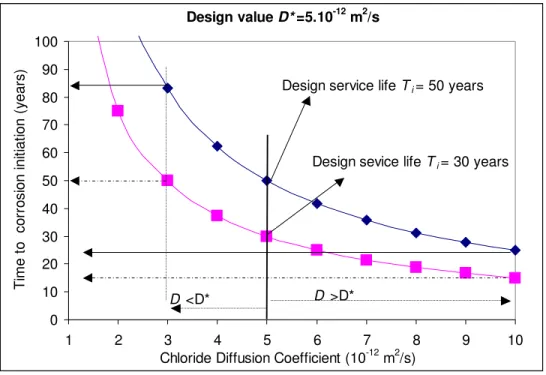
Pseudo Case-Study #1:
Suppose two reinforced concrete structures are designed with D= 0.5·10−11m2/s for a design
time-to-corrosion initiation (or design service life) Ti of 50 years and 30 years, respectively. For D varying from
the design value, say from 10−12 m2/s to 10−11 m2/s, Figure 6 shows how the design service life can be
influenced. If D is increased to 10−11 m2/s, Figure 6 shows that the service life will be reduced to 25 years
and 15 years, respectively. If D is decreased to 3·10−12 m2/s, the service life will be extended to 83 years
and 50 years, respectively. Considering this range of D as feasible in practice, D can be considered as an
effective parameter to control the service life Ti of concrete structures.
4.3.2 Sensitivity to concrete cover depth
Equation (21a) shows the sensitivity S(dc) of Ti to dc, and the correlation between ΔTi/Ti and Δdc/dc is plotted in Figure 5.
1. For small variations of dc less than 10%, S(dc) is approximately equal to 2, i.e. a 10% increase in dc will
increase Ti by 21%.
2. The increase and decrease in Ti are asymmetrical with dc , i.e. an increase in dc will induce a much
greater increase in Ti than a decrease of dc for the same percentage, e.g. a 50% increase in dc will increase
Ti by 125%, while a decrease in dc by 50% will reduce Ti by 75%.
3. Compared to D, dc has a larger impact on Ti, e.g. the variations of dc for ±50%, (which is a small variation in practice), could lead to variations in Ti from –75% to +125%.
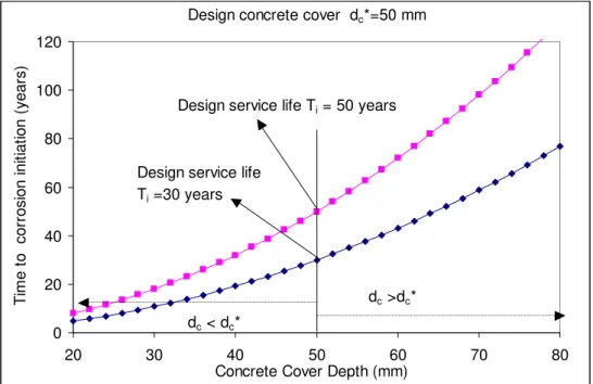
Pseudo Case-Study #2:
Suppose two reinforced concrete structures are designed with a concrete cover depth dc =50 mm for a
design service life Ti of 50 years and 30 years, respectively. Figure 7 shows how the design value of Ti
can be changed by varying the design value of dc between 20 mm to 80 mm. If the value of dc is 20 mm,
Ti will be reduced to 8 and 4.8 years, respectively; if the actual cover is 80 mm, Ti will be increased to 128
and 77 years, respectively.
4.3.3 Sensitivity to surface chloride concentration
As noted before, the variation of ΔTi / Ti with ΔCs /Cs is a function of Cth and Cs. Using the base or mean values of Cs given in Table 1 with Cth =0.52 kg/m3 (case of conventional carbon steel), the variations of
ΔTi / Ti with ΔCs /Cs are illustrated in Figure 8 for the four environmental exposures identified earlier. From Figure 8, the following observations can be made:
1. The variations of ΔCs /Cs from each mean value are from −100% to +33%, ±32%, ±11%, and ±20%, for the light, moderate, high, and severe conditions, respectively. These variations will yield variations in
Ti of −25% to ∞, −18% to 40%, −6% to 7%, −9% to 12%, respectively, for the four exposures. For example, a concrete structure exposed to a moderate environment can be estimated to have a Cs=3.5
kg/m3, if an accurate value is unknown. Since this estimated mean value is associated with a variation
range of ±32%, the resulted variation in Ti will be from –18% to 40%. It means that if the design service life is Ti=50 years, the actual Ti could range from 40 to 70 years.
2. The variations in Ti are more significant for the lighter exposure conditions. Under different exposure
conditions; Ti is increased more significantly by decreasing Cs for light exposure conditions, e.g. a 50%
decrease in Cs would extend the time to onset of corrosion by 261%, 95%, 69%, and 51% for light,
moderate, high, and severe conditions, respectively.
3. A decrease in Cs will induce a much greater increase in Ti than an increase in Cs, e.g., for carbon
100% increase in Cs only decreases Ti by 30%.
4. The higher the reduction in Cs, the higher the increase in Ti , e.g., for carbon reinforcing steel under a
high exposure condition, a 50% decrease in Cs increases Ti by 69%, however, a 70% decrease in Cs
increases Ti by as much as 179%.
Polynomials are used to regress the correlation between Ti /Δ Ti and ΔCs /Cs. After trial-and-error, their correlation can be fitted precisely by a 6th-order polynomial, for –50% <ΔCs /Cs<50%:
m s s m m i i C C T T ] [ B 6 0 Δ = Δ
∑
= (24)where the coefficients Bm are listed in Table B in Appendix.
4.3.4 Sensitivity to chloride threshold level
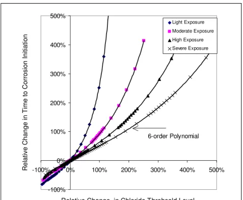
The variations ΔCth /Cth associated with the mean values Cth for each of the four types of steel (Table 2) are used to calculate the variations induced in Ti, for each of the four exposure conditions, if applicable
(assuming Cth ≤ Cs ). The variations of ΔTi / Ti with ΔCth /Cth are also illustrated in Figure 9 for black carbon steel under four exposure conditions. The results can be summarized as follows:
1. Assume Cth =0.52 kg/m3 for carbon steel, if an accurate value is not available (often the case). Since
this mean value is associated with a variation range of ±40%, the variations associated with Ti, will be −40% to 60%, −28% to 32%, −26% to 24%, and −24% to 19%, for light, moderate, high, and severe exposure conditions, respectively. This means if the design service life is Ti=50 years, the actual Ti could
range from 30 to 80 years for a light exposure condition.
2. The closer Cth is to Cs, the more Ti is sensible to Cth. In other words, the higher the value of Cth, the
more sensible Ti is to Cth. This is also verified by comparing different types of steels, e.g. for severe
corrosion exposure Cs=7.4, the variation associated with carbon steel, micro-composite steel, and SS304
3. An increase in Cth will induce a similar amount of change in Ti as a decrease in Cth , e.g. under a high
exposure condition, a 50% change of Cth changes Ti approximately by 30%.
4. The increase rate of Ti by increasing Cth is higher for larger increases, e.g. under a high exposure
condition, e.g., a 100% increase in Cth increases Ti by 69%, while a 300% increase in Cth increases Ti by
as much as 280%. It means that if the carbon steel is replaced by a steel with 3 times higher corrosion
resistance (SS304 is 5 times more corrosion resistant), Ti will be increased by 3 times. Therefore,
increasing of Cth can be considered as an effective measure to increase Ti. Under different environmental
exposures conditions; Ti is increased significantly by increasing Cth under lighter exposure condition, e.g.
a 50% increase in Cth would extend Ti by 260 %, 100%, 69%, and 36% for light, moderate, high, and
severe conditions, respectively. It means the effectiveness of using a more corrosion resistant steel will be
lowered with the increasing severity of environmental exposure.
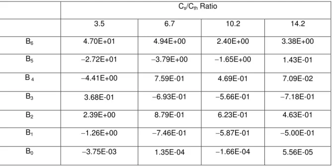
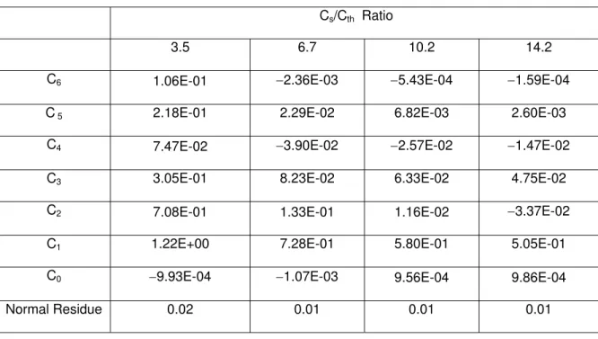
Similarly, polynomials are used to regress the correlation between ΔTi / Ti and ΔCth /Cth for carbon steel. After trial-and-error, this relationship can be fitted by a 6th-order polynomial, for –100%<ΔTi / Ti <400%:
m th th m m i C C C T Ti ] [ 6 0 Δ = Δ
∑
= (25)where the coefficients Cm are listed in Table C in the Appendix.
5. SUMMARY AND CONCLUSIONS
The sensitivity of time to corrosion initiation of the reinforcing steel to the four governing parameters of
the diffusion-based corrosion initiation model, namely the cover depth, chloride diffusivity, surface
chloride concentration and chloride threshold level was investigated. The variations in time to onset of
corrosion induced by realistic variations of the four governing parameters were determined. These results
have important applications in both modeling and practice:
1. The sensitivities of the time to corrosion initiation to concrete cover and chloride diffusion coefficient
cover depth has a higher impact on time to onset of corrosion than does the diffusion coefficient.
2. Considering a feasible range of chloride diffusion coefficients that is relatively easy to achieve in
practice for normal concrete, say from 10−12 m2/s to 10−11 m2/s, decreasing the chloride diffusion
coefficient is considered as an effective measure of extending the time to onset of corrosion. A 50%
decrease in the chloride diffusion coefficient increases the time to corrosion by 100%. Increasing the
concrete cover is an even more effective parameter than chloride diffusion coefficient, since a 50%
increase of concrete cover increases the time to onset of corrosion by 125%.
3. The sensitivity of the time to corrosion to the surface chloride content is a function of the ratio of
surface chloride content and chloride threshold of the steel. A 50% decrease in surface chloride content
would extend the time to onset of corrosion by 261%, 95%, 69%, and 51% in light, moderate, high, and
severe conditions, respectively.
4. The sensitivity of the time to corrosion to the chloride threshold level is a function of the ratio of
surface chloride content and chloride threshold of the steel. Considering only the “intrinsic” variations
(±40%) associated with conventional black carbon steel that are mainly caused by the heterogeneous nature of concrete materials, the variation in time to onset of corrosionwill be −40% to 60%, −28% to 32%, −26% to 24%, and −24% to 19%, for light, moderate, high, and severe exposure conditions, respectively. Comparing different corrosion resistant steels, the sensitivity is higher for more corrosion
resistant steels with higher chloride thresholds. In practice, increasing chloride threshold is an effective
measure to increase the time to onset of corrosion, but the effectiveness of using a more corrosion
resistant steel will be lowered with the increasing severity of the exposure, e.g. a 50% increase in chloride
threshold will extend the time to onset of corrosion by 260 %, 100%, 69%, and 36% for light, moderate,
high, and severe conditions.
In summary, a sensitivity analysis was presented in this paper to quantify the error in the predicted time to
high levels of uncertainty. The impact of each design parameter on the service life of concrete structures
that is critical for a durable design was also evaluated. The results of this sensitivity analysis can be used
as a guide for the design of durable concrete structures build in chloride-laden environments and for the
optimization of inspections and priorities of data collections.
6. NOTATION
C(x,t)= concentration of chlorides in concrete at depth x and time t;
Cs= surface chloride concentration
Cth= threshold chloride concentration for initiation of corrosion of reinforcing steel;
D = chloride diffusion coefficient into concrete;
dc= depth of concrete cover to the reinforcement;
Sj =S(Xj)= normalized sensitivity coefficient of time to corrosion to parameter Xj;
Shj =Sh(Xj)= normalized high-order sensitivity coefficient of time to corrosion to parameter Xj;
t = time (age);
Ti= time to initiation of corrosion of reinforcing steel;
Xj= jth parameter of the model;
Xj0= base (or mean) value of jth parameter of the model;
Xj*= design value of parameter Xj;
X= vector of input variables;
ΔXj= variation of Xj form its base value.
REFERENCES
[1] Alonso, C., Andrade, C., Castello, M., and Castro, P. (2000), Chloride threshold values to depassivate
reinforcing bars embedded in a standardized OPC mortar, Cement and Concrete Research, 30, pp.
[2] ASTM A 615/A 615M-01b, (2002), “Standard Specification for Deformed and Plain Billet Steel Bars
for Concrete Reinforcement,” ASTM International, West Conshohocken, Pa.
[3] Bamforth, P.B., and Price, W.F., An International Review of Chloride Ingress Into Structural
Concrete. Transport Research Laboratory Report 359, Scotland, 1997.
[4] Bentz, D. P., Influence of silica fume on diffusivity in cement based materials, II. Multi-scale
modeling of concrete diffusivity, Cement and Concrete Research, 2000, 30, pp. 1121-1129.
[4] Boddy, A., Bentz, E., Thomas, M.D.A., and Hooton, R.D., An overview and sensitivity study of a
multimechanistic chloride transport model,” Cement and Concrete Research, 1999, 29, pp.827-837.
[6] Cady, P.D., and Weyers, R.E. , Chloride penetration and deterioration of concrete bridge decks.”
Cement, Concrete and Aggregates, 1983, 5(2), 81-87.
[7] Crank, The mathematics of diffusion, 2nd edition, Clarendon press, Oxford, 1975.
[8] Gouda V.K., Corrosion and corrosion inhibition of reinforcing steel. British Corrosion Journal, 1970,
5, p. 198.
[9]Gonzalez, J. A., Algaba, S. and Andrade, C., “Corrosion of reinforcing bars in carbonated concrete,”
British Corrosion Journal, 1980, 15 (3), pp. 135–139.
[10] Kropp, J.,and Hilsdorf, H.K (eds.). Performance Criteria for Concrete Durability. RILEM Report 12,
E& FN Spon, London,1995.
[11] Lounis, Z., Siemes, A.J.M., Lacasse, M., and Moser, K. Further steps towards a quantitative
approach to durability design, in: Materials and Technologies for Sustainable Construction, CIB World
Congress, Gävle, Sweden, 1998, pp. 315-328.
[12] Lounis, Z. Reliability-based life prediction of aging bridge decks. In Life Prediction and Aging
Management of Concrete Structures, Naus, D. (ed.), RILEM Publications, 2000, France, pp.229-238.
[13] Lounis, Z. (2004). Uncertainty modeling of chloride contamination and corrosion of concrete bridge.
In Applied Research in Uncertainty Modeling and Analysis, Attoh-Okine, N.O, and Ayyub, B (eds.),
Springer, Chapter 22, pp. 491-511.
1987.
[15]Rosenberg, A., Hansson C.M., and Andrade, C. (1989). Mechanisms of corrosion of steel in concrete,
in: Materials Science of Concrete I, J. Skalny (ed.), The American Ceramic Society, Inc., Westerville,
OH, pp.285-313.
[16] Thomas, M. D. A and Bamforth, P. B. Modeling chloride diffusion in concrete- effect of fly ash and
slag. Cement and Concrete Research, 1999, 29, pp. 187-495.
[17] Trejo, D. and Pillai, R. G., Accelerated Chloride Threshold Testing—Part I: ASTM A 615 and A 706
Reinforcement. ACI Materials Journal, 100 (6), 2003, pp 519-527.
[18] Trejo, D. and Pillai, R. G., Accelerated Chloride Threshold Testing—Part II: Corrosion-Resistant
Reinforcement. ACI Materials Journal, 101 (1), 2004, pp 57-64.
[19] Tuutti, K., Corrosion of steel in concrete, CBI Research Report 4:82, Swedish Cement and Concrete
Research Institute, Stockholm, 1982.
[20] Tuutti, K, Chloride induced corrosion in marine concrete structures, in: Durability of Concrete on
Saline Environment, Uppsala, 1996, pp. 81-93.
[21] Saltelli, A., Tarantola, S., and Campolongo, F. Sensitivity analysis as an ingredient of modeling.
Statistical Science, 2000, 15 (4), pp. 377-395.
[22] Stratfull, R. F., The corrosion of steel in a reinforced concrete bridge,” Corrosion, 13, March, 1956,
pp. 173-178.
[23] Weyers, R. E., Prowell B. D., Sprinkel, M. M., Concrete Bridge protection, repair, and rehabilitation
Figure Captions
Fig. 1. Service life of concrete structures subjected to corrosion (adapted from Tuutti 1982)
Fig. 2. Relationship between time to corrosion initiation and diffusion model parameters
Fig. 3. Incorporation of parameter uncertainty in model prediction
Fig. 4. Sensitivities of Ti to D, dc, Cs, Cth as functions of Cs/Cth ratio
Fig. 5. Sensitivities of Ti to chloride diffusion coefficient and concrete cover depth
Fig. 6. Impact of diffusion coefficient on corrosion initiation time
Fig. 7. Impact of concrete cover depth on corrosion initiation time
Fig.8. Impact of surface chloride concentration on corrosion initiation time
Time Degree of corrosion
Acceptable degree
Initiation Time Propagation Time
Service Life
Cl− ,CO2, penetration
O2, RH,
Temperature, Onset of Corrosion
0 20 40 60 80 100 0 0.1 0.2 0.3 0.4 0.5 0.6 0.7 0.8 0.9 1
C
th/C
s 4T i D/ dc 2 12-order polynomials normr= 0.0166Reinforced concrete structure
Environment:Surf..
chloride level (Cs)
Concrete Type: Chloride diffusion coefficient (D)
Steel Type: Chloride
threshold level (Cth)
Structure: Cover
depth (dc)
Diffusion-Based Model
Corrosion Initiation Time (Ti)
Uncertainty in Cs, Cth, D, dc
Sensitivity Analysis of Ti
Uncertainty in Ti Parameter Ranking
Effective decision-making for design, inspection and maintenance
-4 -3 -2 -1 0 1 2 3 4 1 2 3 4 5 6 7 8 9 10 Cs/Cth Ratio
Fi
rs
t-or
der
S
ens
it
iv
it
y
dc D Cs Clth-100 -50 0 50 100 -100 -50 0 50 100 Relative variation of D or dc(%) R e la tive Chan ge in tim e t o co rrosi on in itiat ion ( % ) D dc
0 10 20 30 40 50 60 70 80 90 100 1 2 3 4 5 6 7 8 9 10
Chloride Diffusion Coefficient (10-12 m2/s)
T im e to c o rro s io n i n it ia ti o n (y e a rs ) Design value D* =5.10-12 m2/s
Design service life Ti= 50 years
Design sevice life Ti= 30 years
D <D* D >D*
0 20 40 60 80 100 120 20 30 40 50 60 70 80
Concrete Cover Depth (mm)
T ime to c o rr o s io n i n it ia ti o n ( y e a rs )
Design concrete cover dc*=50 mm
Design service life Ti = 50 years
Design service life Ti =30 years
dc < dc*
dc >dc*
-100% -50% 0% 50% 100% 150% 200% 250% 300% -50% -40% -30% -20% -10% 0% 10% 20% 30% 40% 50% Relative Change in Surface Chloride Concentration
Relative Change in Time to Corrosion Initiation
Light Exposure Moderate Exposure High Exposure Severe Exposure 6-order Polynomial
-100% 0% 100% 200% 300% 400% 500% -100% 0% 100% 200% 300% 400% 500%
Relative Change in Chloride Threhsold Level
Relativ e Cha nge in Time to Co rrosion Initia tion Light Exposure Moderate Exposure High Exposure Severe Exposure 6-order Polynomial
APPENDIX
Table A: Coefficients of polynomial in Eq.5
A6 =3.87E+06 A12 =1.50E+06 A5 =−1.04E+06 A11 =−7.45E+06 A4 =1.95E+05 A10 =1.66E+07 A3 =−2.40E+04 A9 =−2.11E+07 A2 =1.85E+03 A8 =1.75E+07 A1 =−7.59E+01 A7 =−9.90E+06
A0 =1.78E+00 Normal Residue 0.000001
Table B: Coefficients of polynomial in Eq. 24
Cs/Cth Ratio
3.5 6.7 10.2 14.2
BB6 4.70E+01 4.94E+00 2.40E+00 3.38E+00
BB5 −2.72E+01 −3.79E+00 −1.65E+00 1.43E-01
BB 4 −4.41E+00 7.59E-01 4.69E-01 7.09E-02
BB3 3.68E-01 −6.93E-01 −5.66E-01 −7.18E-01
BB2 2.39E+00 8.79E-01 6.23E-01 4.63E-01
BB1 −1.26E+00 −7.46E-01 −5.87E-01 −5.00E-01
Table C: Coefficients of polynomial in Eq. 25
Cs/Cth Ratio
3.5 6.7 10.2 14.2
C6 1.06E-01 −2.36E-03 −5.43E-04 −1.59E-04
C 5 2.18E-01 2.29E-02 6.82E-03 2.60E-03
C4 7.47E-02 −3.90E-02 −2.57E-02 −1.47E-02
C3 3.05E-01 8.23E-02 6.33E-02 4.75E-02
C2 7.08E-01 1.33E-01 1.16E-02 −3.37E-02
C1 1.22E+00 7.28E-01 5.80E-01 5.05E-01
C0 −9.93E-04 −1.07E-03 9.56E-04 9.86E-04
Table Titles
Table 1. Sensitivity of time to corrosion initiation to environmental exposure for carbon steel
Table 2 Sensitivity of corrosion initiation time to chloride threshold level for different exposures
Table 1. Sensitivity of corrosion initiation time to environmental exposure for carbon steel
Condition Low (kg/m3) Moderate (kg/m3) High (kg/m3) Severe (kg/m3) Range 0 <Cs < 2.4 2.4 < Cs < 4.7 4.7 < Cs < 5.9 5.9 < Cs< 8.9 Mean value 1.8 3.5 5.3 7.4 Variation from mean value −100% to 33% −32% to 32% −11% to 11% −20% to 20% Variation in Ti −25% to
∞
−18% to 40% −6% to 7% −9% to 12% * Note 1 Kg/m3 = 0.276% of cement weight for normal weight concreteTable 2. Sensitivity of corrosion initiation time to chloride threshold level for different exposures
Variations in chloride threshold level Steel Type & Environment Conventional carbon steel (kg/m3) Micro-composite steel-MMFX (kg/m3) Stainless steel SS304 (kg/m3) Stainless steel SS216LN (kg/m3) Range 0.30 <Cth< 0.71 3.8< Cth <5.3 4.1< Cth <6.0 9.5< Cth <12.0 Mean value 0.52 4.6 5.0 10.8 Variation from mean value * −40% to 40%* −16% to 16% −19% to 19% −12% to 12% Variations in corrosion initiation time
Light Cs = 1.8 kg/m3 −40% to 60% + + + Moderate Cs = 3.5 kg/m3 −28% to 32% + + + High Cs = 5.3 kg/m3 26% to –24% −80% to + −84% to + + Severe Cs = 7.4 kg/m3 −24% to 19% −40% to 96% −50% to 400% +