Automatic modeling of machining processes

Automatic Modeling of Machining Processes

by

Chetan Sharma

B.S. in Electrical Engineering and Computer Science, Massachusetts

Institute of Technology (2019)

Submitted to the Department of Electrical Engineering and Computer

Science

in partial fulfillment of the requirements for the degree of

Master of Engineering in Electrical Engineering and Computer Science

at the

MASSACHUSETTS INSTITUTE OF TECHNOLOGY

February 2021

c

○ Massachusetts Institute of Technology 2021. All rights reserved.

Author . . . .

Department of Electrical Engineering and Computer Science

September 4, 2020

Certified by . . . .

Neil Gershenfeld

Director & Professor at Center for Bits and Atoms

Thesis Supervisor

Accepted by . . . .

Katrina LaCurts

Chair, Master of Engineering Thesis Committee

Automatic Modeling of Machining Processes

by

Chetan Sharma

Submitted to the Department of Electrical Engineering and Computer Science on September 4, 2020, in partial fulfillment of the

requirements for the degree of

Master of Engineering in Electrical Engineering and Computer Science

Abstract

3 axis CNC milling is a ubiquitous manufacturing method in industry due to its ver-satility and precision. The fundamental parameters that dictate cutting performance ("speeds, feeds, and engagement") must be manually set by the machine programmer; proper operation therefore relies heavily on operator skill. In this thesis, an intelligent CNC controller is presented that uses low-cost sensors to fit an analytical model of cutting forces. The analytical nature of this model allows for favorable convergence characteristics and low computational costs. This is used to optimize cutting feeds with respect to process constraints for future movements; as more data is collected, the model continuously reinforced. This intelligent controller therefore abstracts out some of the complexities of machining and makes the process more approachable. Thesis Supervisor: Neil Gershenfeld

Acknowledgments

A large thanks goes to my mentor Jake Read, my supervisor Neil Gershenfeld, and the many researchers at the Center for Bits and Atoms. Being surrounded by brilliant scientists was as inspiring as it was intimidating!

An additional thanks goes to Ted Hall from Shopbot for providing me with CNC equipment during the COVID-19 crisis. This thesis would be strictly impossible without his help.

One more thanks goes to the Yang family for providing me with a place to live during the crisis; their kindness cannot be understated.

A final thanks goes to the numerous geckos that inhabited my garage workshop while I worked on my thesis. They contributed nothing, but they were very cute.

Contents

1 Introduction 13

1.0.1 The Value of Abstraction . . . 13

1.0.2 Difficulties Associated with Milling Abstractions . . . 14

1.0.3 Self-Improving Analytical Model-Based Controllers . . . 15

1.0.4 The Value of Simplicity . . . 15

1.1 Background . . . 16

1.1.1 Milling Models . . . 16

1.1.2 Feed Rate Scheduling . . . 17

1.1.3 Feedback . . . 17

1.1.4 Process Optimization / Failure . . . 18

1.2 Prior Work . . . 18

2 Proposed System 21 2.1 The Milling Model . . . 22

2.2 Regression . . . 25

2.3 Failure Models . . . 25

2.3.1 Deflection Model . . . 26

2.3.2 Tool Breakage Model . . . 27

2.3.3 Spindle Load Model . . . 28

2.4 Optimization . . . 28

2.5 Model Bootstrapping and Data Persistence . . . 29

2.6 Hardware . . . 30

2.6.2 Uniaxial Tool Force Dynamometer . . . 32

3 Evaluation 35 3.0.1 Experimental Setup . . . 35

3.1 Model Fit Performance . . . 36

3.2 Optimization Performance . . . 36 3.3 System Adaptability . . . 36 4 Conclusion 43 4.1 Future Work . . . 43 4.1.1 Modeling Improvements . . . 44 4.1.2 Workflow Improvements . . . 45 4.2 Final Thoughts . . . 45

List of Figures

1-1 Traditional machining workflow . . . 14

1-2 Machining workflow described in this work . . . 16

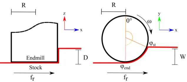
2-1 Diagram of the flat-milling process . . . 22

2-2 Diagram of milling forces . . . 24

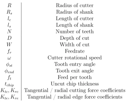
2-3 Diagram of an endmill. See table 2.1 for variable definitions . . . 26

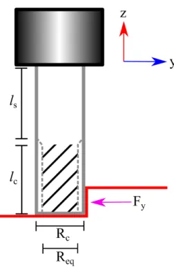
2-4 Diagram of bootstrapping process . . . 30

2-5 Machine used for experimentation . . . 31

2-6 Tool force dynamometer implementation . . . 33

2-7 Servo-equipped spindle implementation . . . 33

3-1 Model fit for spindle torques . . . 37

3-2 Model fit for cutting forces . . . 37

3-3 Model fit for spindle torques when asked to extrapolate feeds above 0.004 38 3-4 Model fit for cutting forces when asked to extrapolate feeds above 0.004 38 3-5 Convergence of model to ground-truth data over successive cuts . . . 39

3-6 Model fit after all cuts were made (i.e "in hindsight") . . . 39

3-7 Convergence examples for successful tests . . . 41

List of Tables

2.1 Variable definitions . . . 23 3.1 Materials tested & endmill diameters used. . . 40

Chapter 1

Introduction

CNC1 _{milling is a staple of modern manufacturing. Since its genesis at the MIT} Servomechanisms laboratory, CNC milling has grown into a multi-billion dollar in-dustry. The high accuracy and versatility of these machines enable them to be used in situations that call for complex geometry and tight tolerances. Process constraints are minimal compared to other manufacturing methods, so CNC milling machines find uses in a variety of industries (mold-making, prototyping, aerospace, commercial products, etc.) [1].

1.0.1

The Value of Abstraction

Abstraction is a key component of the growing personal fabrication movement. The complexity of creating anything can become overwhelming when the minutiae of its creation must be considered; removing this barrier lets creators focus on the "what" instead of the "how". Consider the recent spike in hobbyist FDM2 _{3D printing; by} reducing fabrication to a "click-and-watch" process, 3D printers have enabled even novice makers to create almost anything with basic fabrication knowledge [2].

Much of the CNC mill’s appeal can be attributed to the strength of the abstraction it provides. The sequence of motions required to machine a part is typically generated

1_{Computer Numeric Control}

Figure 1-1: Traditional machining workflow

directly from a CAD3 _{model using CAM software. In this software a user defines a} tool to use, a feature to recreate on the model, and a few parameters that define how this is done. The software then translates these directives into G-Code4 _for the physical machine. Figure 1-1 depicts this workflow. In this sense, CNC milling provides a way of creating a functional object without worrying about the "how".

1.0.2

Difficulties Associated with Milling Abstractions

This abstraction, however, is highly imperfect. The complex nature of the milling process leaves many avenues for failure. Too high of a cutting speed can melt the material; too high of a feed rate can overpower the machine or snap the cutting tool. Modern CNC milling workflows leave these critical variables (speed, feed, engage-ment) as an exercise for the machine operator - and the operator, in turn, is left to rely on scant resources5_{, audible cues, and intuition. Modern CNC milling fails to} ab-stract out human judgement and often places itself out of reach for the inexperienced machinist.

The difficulty of abstracting out these variables comes from the natural inscrutabil-ity of the machining process. A complex mixture of thermal, tribological, static, and

3_{Computer Aided Design; an abstract computer representation of a physical part} 4_{A basic text-based language used to provide instructions to CNC machines}

5_{Tool manufacturers provide recommendations for feeds and speeds for each tool-material}

dynamic mechanisms govern cutting. Tractable models of milling in academia rely on empirically determined constants. These constants are typically specific to only one tool-material combination and can vary with the cutting environment; the introduc-tion of coolant or the use of a stiffer machine can result in entirely new values. With no way of obtaining these constants, CNC operators generally resort to using a com-bination of simpler heuristics and intuition to select parameters. A better solution is clearly in order.

1.0.3

Self-Improving Analytical Model-Based Controllers

In this thesis, an intelligent machine controller is developed with the goal of abstract-ing out the complexities of parameter selection. This new workflow is depicted in fig-ure 1-2. Machining constraints are automatically determined using easily-measurable machine & tool properties. Feedback from a low-cost 1D tool-force dynamometer and a current-sensing spindle is used to fit cutting force coefficients to a simple analytical model of flat end-milling in real time. This model is used to estimate a feed rate that will simultaneously maximize productivity and obey the previously calculated constraints. This model-based feedback approach mimics what a human operator does. Intuition is replaced by a tractable mathematical model; audible and visible indications of proper machining are replaced by ground-truth sensor readings. This intelligent controller abstracts out some of the complexity of tuning parameters and permits the operator to treat the machine as more of a black box.

1.0.4

The Value of Simplicity

This thesis was completed during the COVID-19 pandemic in the absence of a real machine shop with limited funding. These conditions made simplicity an implicit requirement; complex mechanisms and sensors were simply unobtainable. While this thesis could not explore more refined testing and manufacturing methods, the com-pletion of this system despite limited resources proves that intelligent controllers can be implemented without exotic hardware.

Figure 1-2: Machining workflow described in this work

1.1

Background

1.1.1

Milling Models

Both numerical and analytical models exist for predicting milling forces. While nu-merical models can achieve higher accuracy, the simplicity of the analytical models makes them more suitable for this system.

Many models derive cutting forces from a relationship between uncut chip thick-ness6 _{as well as radial and tangential cutting pressures. Integrating these pressures} over the appropriate bounds along cutting edges yields cutting forces and torques as a function of time. Tool deflection, runout, and non-perpendicularity can be accounted for if desired.

Two common relationships between uncut chip thickness and cutting pressures are defined by the edge-force model and the exponential-model. The linear-edge force model assumes that cutting pressures can be divided into a "cutting" component that varies linearly with chip thickness and an "edge" component that is unchanging. The exponential model is an expansion of the former wherein the cutting

force coefficients themselves vary exponentially with average chip thickness. All of these relationships are typically found through linear regressions on actual cutting data.

Budak et al. has described and verified the effectiveness of linear-edge force models for end milling [3] [4]; due to their simplicity, they will be used for this work. Similar models exist for ball milling [5] and twist drilling [6], so the system described in this thesis could be adapted to other forms of tooling.

1.1.2

Feed Rate Scheduling

When milling forces are known, they can be used to adjust feedrates as cutting con-ditions change. Feedrate scheduling refers to this practice; it is most often used to compensate for a fluctuating level of tool engagement. Scheduling, however, requires an accurate model that relates cutting conditions to process outputs. These models rely on empirical coefficients that are specific to each material and tool, so scheduling is limited to applications where the cost of collecting these coefficients can be justified.

1.1.3

Feedback

Feedback from sensors can be used to perform feedrate scheduling in response to actual cutting conditions. Traditional PI controllers7 have been used, but they can struggle to cope with rapidly changing process inputs without a feedforward element. More advanced systems utilize learning-based controllers to respond to these changes faster. Fuzzy controllers, GA controllers8_{, and ANN controllers}9 _{have been explored} in other works [7].

Force feedback is typically obtained from a commercial piezoelectric tool-force dynamometer. While accurate, these devices are expensive; they must exhibit high stiffness and avoid cross-coupling between axes. Production machines lack this in-strumentation for reasons of cost and robustness.

7_{Proportional integral} 8_{Genetic algorithm} 9_{Artificial neural network}

Spindle-load based feedback has been used with some success. K. Dunwoody uses spindle-load measurements directly from a commercial machine to estimate cutting force coefficients [8]. D. Kim et al. uses raw current readings from a hall-effect board paired with an empirically-found relation to find cutting torques [9]. Finding feed-axis cutting forces through motor currents proved to be more difficult due to the complex tribology associated with way motion.

1.1.4

Process Optimization / Failure

A typical objective in milling is to remove material at the maximum permitted rate while avoiding tool or machine failure. Failure modes for tooling include tool breakage (governed by brittle failure laws in carbide tooling), tool deflection (governed by static mechanics), and spindle failure (governed by the motor driving the spindle). Other failure mechanisms such as overheating and regenerative chatter also exist but will be considered out-of-scope for this thesis.

J.A Nemes et al. [10] obtained the Weibull parameters for carbide tool fracture; those parameters will be used in this work. Calculating endmill deflection can be difficult due to the complex geometry present. Simplified models have been proposed as alternatives. One work found that an endmill’s fluted portion can be approximated by a cylinder with 80% of its diameter [11]. Another used FEA data to create a simplified empirical formula to describe deflections more accurately [12].

1.2

Prior Work

Systems described by both U. Zuperl et al. and D. Kim use a fuzzy logic controller to schedule feedrates in real-time [13] [9]. In both implementations, hand-picked fuzzy logic rules are used to convert measured force errors to feed commands. While these controllers are stable, they do not employ feedforward predictions and therefore require finite time to respond to force changes [9]. Finite response times can lead to tool breakage and form errors. Some degree of operator skill is also required to build and tune the controller.

U. Zuperl et al. also uses a feedforward neuro-fuzzy system in a separate publica-tion [14]. A neuro-fuzzy model of cutting and a ANFIS10_{model of tool flank wear are} used to find optimal feedrates. Data from the cutting process is then used to correct for errors in force by means of a separate neural controller. This architecture, while highly accurate, incurs a great deal of complexity and requires expensive sensors for data collection. Its implementation is therefore limited to higher-end machines.

All of the above systems model the cutting process by means of a universal func-tion approximator. These approximators are not guaranteed to capture the exact relationship between input and output variables. While this is acceptable when inter-polating between captured data points, it becomes more problematic when the system is asked to extrapolate. A large quantity of data is required to bootstrap a function approximator and ensure that the model does not diverge from the ground-truth at extreme values.

Chapter 2

Proposed System

The machining system proposed in this thesis attempts to improve on prior systems in terms of simplicity, cost, and extrapolative performance. This system consists of four interoperating components:

∙ An analytical model of the milling process ∙ An analytical model of milling failure ∙ A nonlinear optimizer

∙ A milling machine instrumented with sensors

The analytical model of the milling process is parameterized by coefficients specific to the tool-material combination being used; it relates cutting conditions to cutting torques and forces. The analytical model of failure uses the force model’s output to calculate if the milling process will fail. The nonlinear optimizer uses both of these models to find cutting parameters that will result in the highest MRR1_{. while} keeping milling forces within safe limits. These cutting parameters are given to the path planner and machine. The resulting cutting torques and forces are captured by sensors and used to improve the coefficients defining the milling model. This cycle allows cutting parameters to be optimized with a self-improving model.

Figure 2-1: Diagram of the flat-milling process

2.1

The Milling Model

A model is required that relates fundamental cutting parameters to average cutting torques and radial force vectors. This model will be formed under the assumption that a flat-nose helical endmill is being used for climb machining. Figure 2-1 and table 2.1 describe key variables. Similar models exist for ball-nose machining but will not be considered in this work [5].

The linear-edge force model will be used in this work. This choice is motivated by multiple factors:

∙ The model is purely analytical and can be evaluated without costly numerical methods. This makes it possible to implement this system with less computa-tional overhead.

∙ Despite its simplicity, the model describes average torques and forces well enough for effective optimization.

∙ The model is linear, so familiar linear regression techniques can be applied. ∙ The model has very few parameters and converges much faster than its

function-approximator counterparts. It also extrapolates very well.

In this model, cutting forces are derived from radial and tangential pressures that develop along cutting edges (see figure 2-2). One component of these cutting pressures

𝑅 Radius of cutter 𝑅𝑠 Radius of shank 𝑙𝑐 Length of cutter 𝑙𝑠 Length of shank 𝑁 Number of teeth 𝐷 Depth of cut 𝑊 Width of cut 𝑓𝑟 Feedrate

𝜔 Cutter rotational speed

𝜑𝑠𝑡 Tooth entry angle

𝜑𝑒𝑛𝑑 Tooth exit angle

𝑓𝑡 Feed per tooth

𝑡𝑐ℎ𝑖𝑝 Uncut chip thickness

𝐾𝑡𝑐, 𝐾𝑟𝑐 Tangential / radial cutting force coefficients 𝐾𝑡𝑒, 𝐾𝑟𝑒 Tangential / radial edge force coefficients

Table 2.1: Variable definitions

varies linearly with uncut chip thickness and is associated with the energy needed to deform the chip. The other component does not and is associated with the energy needed to force a imperfect cutting edge through the material. Axial cutting pressures will be ignored as they do not have a significant impact on the milling process.

The uncut chip thickness varies with 𝜑 and the feed per tooth. This quantity is linearly related to cutting pressures:

𝑡𝑐ℎ𝑖𝑝 ≈ 𝑓𝑡cos 𝜑 = 2𝜋𝑓𝑟 𝑁 𝜔 cos 𝜑 𝑑𝐹𝑡 = (𝐾𝑡𝑐𝑡𝑐ℎ𝑖𝑝+ 𝐾𝑡𝑒) ⎡ ⎣ − cos 𝜑 sin 𝜑 ⎤ ⎦ 𝑑𝐹𝑟 = (𝐾𝑟𝑐𝑡𝑐ℎ𝑖𝑝+ 𝐾𝑟𝑒) ⎡ ⎣ − sin 𝜑 − cos 𝜑 ⎤ ⎦

For climb cutting, 𝜑𝑠𝑡 and 𝜑𝑒𝑛𝑑 take on the values:

𝜑𝑠𝑡 = 𝜋 − arccos(1 − 𝑊

𝑅) 𝜑𝑒𝑛𝑑 = 𝜋

Figure 2-2: Diagram of milling forces

The average torque induced in the cutter is equal to the integral of the tangential cutting pressures of the teeth that are in contact with the workpiece. Radial cutting pressures make no contributions to torque:

𝜏 = 𝐷𝑁 𝑅 2𝜋 ∫︁ 𝜑𝑒𝑛𝑑 𝜑𝑠𝑡 𝐾te+ 𝐾tc𝑓𝑡 sin (𝜑) = 𝐷 𝑁 𝑅 2𝜋 (︂ 𝐾teacos (︂ 1 −𝑊 𝑅 )︂ +𝐾tc𝑊 𝑓𝑡 𝑅 )︂

Contributions from both tangential cutting pressures and radial cutting pressures need to be combined in order to find cutting forces. The following integral describes forces along X and Y:

𝐹 = 𝐷𝑁

2𝜋

∫︁ 𝜑𝑒𝑛𝑑

𝜑𝑠𝑡

𝑑𝐹𝑡+ 𝑑𝐹𝑟

These equations leave us with four unknown coefficients: 𝐾𝑡𝑐, 𝐾𝑡𝑒, 𝐾𝑟𝑐, and 𝐾𝑟𝑒. These coefficients vary with the material being cut and the tool’s coating, but they do not vary with the tool’s flute count or diameter.

2.2

Regression

The expressions for 𝐹𝑥and 𝐹𝑦 share the same coefficients so only one force component is needed for regression. The model described above has the convenient property of being linear with respect to its coefficients. Because of this, the equations for average torque and average force along the 𝑦 axis can be simplified to the following:

[︁ 𝜏 𝐹𝑦 ]︁ = [︁ 𝐾𝑡𝑐 𝐾𝑡𝑒 𝐾𝑟𝑐 𝐾𝑟𝑒 ]︁ ⎡ ⎢ ⎢ ⎢ ⎢ ⎢ ⎢ ⎣ 𝑋𝜏 1 𝑋𝐹𝑦1 𝑋𝜏 2 𝑋𝐹𝑦2 𝑋𝜏 3 𝑋𝐹𝑦3 𝑋𝜏 4 𝑋𝐹𝑦4 ⎤ ⎥ ⎥ ⎥ ⎥ ⎥ ⎥ ⎦ ⎡ ⎢ ⎢ ⎢ ⎢ ⎢ ⎢ ⎣ 𝑋𝜏 1 𝑋𝜏 2 𝑋𝜏 3 𝑋𝜏 4 ⎤ ⎥ ⎥ ⎥ ⎥ ⎥ ⎥ ⎦ = ⎡ ⎢ ⎢ ⎢ ⎢ ⎢ ⎢ ⎣ 𝐷 𝑁 𝑊 𝑓𝑡 2 𝜋 𝐷 𝑁 𝑅 acos(1−𝑊_𝑅) 2 𝜋 0 0 ⎤ ⎥ ⎥ ⎥ ⎥ ⎥ ⎥ ⎦ ⎡ ⎢ ⎢ ⎢ ⎢ ⎢ ⎢ ⎣ 𝑋𝐹𝑦1 𝑋𝐹𝑦2 𝑋𝐹𝑦3 𝑋𝐹𝑦2 ⎤ ⎥ ⎥ ⎥ ⎥ ⎥ ⎥ ⎦ = ⎡ ⎢ ⎢ ⎢ ⎢ ⎢ ⎢ ⎣ 𝐷 𝑁 𝑓𝑡(𝑊3/2 √ 2 𝑅−𝑊 +𝑅2_acos(𝑅−𝑊 𝑅 )−𝑅 √ 𝑊√2 𝑅−𝑊) 4 𝑅2_𝜋 𝐷 𝑁 𝑊 2 𝑅 𝜋 𝐷 𝑁 𝑊 𝑓𝑡(2 𝑅−𝑊 ) 4 𝑅2_𝜋 𝐷 𝑁√𝑊√2 𝑅−𝑊 2 𝑅 𝜋 ⎤ ⎥ ⎥ ⎥ ⎥ ⎥ ⎥ ⎦

Standard L2 linear regression can then be used to find the coefficient’s values. Since the equations for torque and force share the same set of coefficients, data from both can be used simultaneously in the same regressor (provided that both are rescaled to be closer in magnitude).

2.3

Failure Models

There are multiple ways in which the milling process commonly fails: ∙ Tool breakage

Figure 2-3: Diagram of an endmill. See table 2.1 for variable definitions

∙ Spindle overload

∙ Tool overheating / material melting ∙ Excessive regenerative chatter ∙ Premature tool wear

This system is limited to predicting failure modes that can be derived from torque and force. Tool wear and heat generation come from complex tribological processes while regenerative chatter requires a detailed model of the machine’s frequency re-sponse. Only the first three listed items will be considered in this work.

2.3.1

Deflection Model

Deflection during the cutting process leads directly to dimensional errors in the fin-ished part. The complex geometry of an endmill’s flutes can make it difficult to analytically find deflection under load. Calculations can be simplified by approximat-ing the fluted portion as a cylinder that is 80% of the cutter’s radius [15]. With this

assumption in hand, the endmill can be analyzed as a simple cantilevered beam with a step in diameter. Cutting forces will be reduced to a point load at a distance of

1

2𝐷 from the tip. Deflections along X are aligned with the feed direction and do not contribute to form errors, so deflections along Y will be of primary interest.

𝐼𝑐 ≈ 𝜋(0.8𝑅𝑐)4 4 𝐼𝑠 = 𝜋𝑅4_𝑠 4 𝑀𝑠 = 𝐹𝑦(𝑙𝑐− 𝐷 2) 𝜃𝑠 = 2𝑀𝑠𝑙𝑠+ 𝐹𝑦𝑙2𝑠 2𝐸𝐼𝑠 𝛿𝑠 = 3𝑀𝑠𝑙2𝑠+ 2𝐹𝑦𝐼𝑠3 6𝐸𝐼𝑠 𝛿𝑐 = 𝐹𝑦(𝑙𝑐− 𝐷₂)2(2𝑙𝑐+𝐷₂) 6𝐸𝐼𝑐 + 𝛿𝑠+ 𝜃𝑠𝑙𝑐

Deflections can also come from the machine itself. Linear-elastic deflections are easy to measure (e.g with a dial indicator) so the machine’s deflections will be modeled in this fashion:

𝛿𝑡𝑜𝑡𝑎𝑙 = 𝛿𝑐+ 𝐹𝑦 𝐾𝑚𝑎𝑐ℎ𝑖𝑛𝑒

2.3.2

Tool Breakage Model

Modern flat endmills are made from cemented carbide and behave like a brittle solid. Tool fracture probabilities can therefore be approximated by a Weibull distribution over peak stresses. The Weibull CDF takes the following form:

𝑃𝑓 𝑟𝑎𝑐 = 1 − 𝑒−(

𝜎𝑚𝑎𝑥 𝜆 )

Drawing from experiments run by J.A Nemes et al. [10], 𝜆 and 𝑘 will be assigned values 1566×106 _{MPa and 5.64 respectively. 𝜎}

𝑚𝑎𝑥 will appear either at the boundary between the cutter and the shank or at the boundary between the shank and the collet. The simplifying assumptions used for tool deflection can be applied again to find these stresses.

𝜎𝑐𝑢𝑡,𝑠ℎ = ||𝐹 ||𝑅𝑐(𝑙𝑐− 𝐷₂) 𝐼𝑐 𝜎𝑠ℎ,𝑐𝑜𝑙 = ||𝐹 ||𝑅𝑠(𝑙𝑐+ 𝑙𝑠− 𝐷₂) 𝐼𝑠

2.3.3

Spindle Load Model

Conditions that result in spindle overload depend on the type of spindle motor being used. AC Induction and permanent magnet synchronous motors2 are common motor choices; the latter will be modeled for this work.

If it is assumed that the motor is not near its limiting speed, the maximum torque attainable is equal to:

𝜏𝑚𝑎𝑥 = 𝐾𝜏𝐼𝑚𝑎𝑥

2.4

Optimization

Traditional nonlinear optimization techniques can be used if the optimality of the cutting process is represented as a minimizable function (a "loss" function). The loss function will need to map potential cutting conditions to a measure of optimality. Optimality will be defined as the negative product of a "success" metric and a "success probability" metric. The success metric will be defined as MRR.

The success probability metric will be defined in terms of the failure models

lished earlier. This metric should be continuously differentiable and should drop off steeply if the predicted output of any failure model comes within 90% of its allowable threshold. This is achieved by means of an reversed logistic function.

𝜆 = −𝐿𝑜𝑝𝑡𝐿𝑠𝑢𝑐 𝐿𝑜𝑝𝑡 = 𝐷𝑊 𝑓𝑟 𝐺(𝑥) = 1 − 1 1 + 𝑒−20(𝑥−0.9) 𝐿𝑠𝑢𝑐 = 𝑖 ∏︁ 𝐺(𝐹𝑖,𝑝𝑟𝑒𝑑 𝐹𝑖,𝑚𝑎𝑥 )

A standard nonlinear optimizer can then be used to find the best cutting condi-tions. scipy.optimize.minimize3 _{was used with satisfactory results. Depth-of-cut,} width-of-cut, and feedrate can be optimized simultaneously; spindle speed can also be included if the machine has a provision to prevent tool overheating (i.e flood coolant).

2.5

Model Bootstrapping and Data Persistence

The model described above has no data when instantiated and no predictive power; it therefore cannot be relied upon by the optimizer until it collects sufficient data. To work around this, the system starts cutting with conservative user-set "bootstrap" parameters that are guaranteed to be safe. Data from this bootstrap cut is fed to the model to improve it slightly. The still-unreliable model is then used by the optimizer to find unreliable optimized cutting parameters. The system does not use these unreliable cutting parameters directly; it instead interpolates between the bootstrap parameters and the unreliable parameters. The interpolation initially favors the bootstrap parameters; as more data is collected, it linearly shifts towards the optimized parameters. Figure 2-4 shows the process in detail.

At least two interpolative steps must be taken to guarantee that the linear regres-sion problem is not underdetermined but taking more steps is required in practice

Figure 2-4: Diagram of bootstrapping process

due to sensor noise. Five interpolative steps were used in this implementation. As mentioned before, cutting coefficients are specific to each material / tool com-bination. If a set of tools with a consistent rake angle and surface finish are used on the same material, however, data from all of these tools can be shared. Bootstrapping becomes unnecessary if at least one similar tool has already been used to cut the same material.

2.6

Hardware

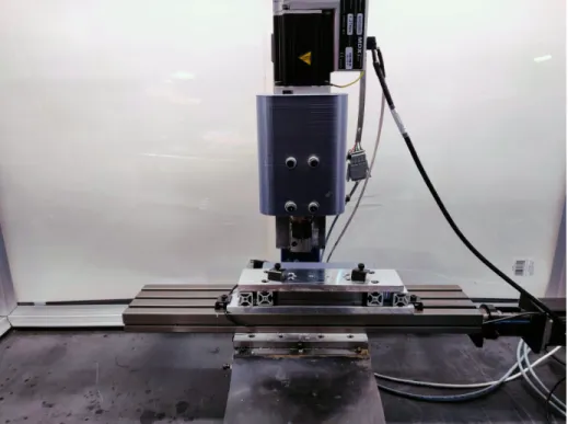
The hardware setup for this system consists of a Taig Tools CNC micro milling ma-chine retrofitted with a torque-sensing spindle and a uniaxial tool force dynamome-ter. The machine is driven by Gecko G250X stepper drivers connected to a GRBL-based controller. The structural loop between the spindle and table has a stiffness of 1.25 × 105 _{N/m. An air blast is used to evacuate chips and prevent the cutter from} overheating.

pan-Figure 2-5: Machine used for experimentation

demic with few available resources. As such, it was especially important that all sensors be low-cost and easy to fabricate.

2.6.1

Torque Sensor

Torque readings can be indirectly acquired by measuring the spindle motor’s RMS phase currents. If the motor uses a well-implemented FOC4 algorithm, a majority of this current will be quadrature current. This enables motor torques to be calculated using the motor’s torque constant, 𝐾𝑇.

An Applied Motion Products MDXK62GN3 servomotor was used in this work. The motor was directly coupled to the spindle to improve sensor bandwidth. Raw current readings from the motor were noisy due to the nature of the internal PID velocity loop; a mean filter w/ outlier removal was used to obtain cleaner readings. The actual spindle is shown in figure 2-7b.

4_{Field Oriented Control; an algorithm used to orient a motor’s electromagnetic field at an optimal}

An off-the-shelf VESC5 connected to a BEI DIH23-30-013Z was also tested but failed to maintain stability during cutting. A reliable FOC algorithm proved to be essential for this application.

A significant amount of motor torque is needed in order to overcome friction and viscous damping present in the spindle. This torque was found to vary with both spindle speed and spindle bearing temperature on the Taig. To compensate for this, no-load spindle currents were briefly measured out-of-cut before each consecutive cut.

2.6.2

Uniaxial Tool Force Dynamometer

Since the model used for this system defines a relationship between the X and Y cutting force components, only one of these components needs to be measured. This greatly simplifies the design of the tool force dynamometer and makes it possible to construct one using off-the-shelf parts.

The tool force dynamometer used for this thesis consists of a base plate and a top plate with a Schneeberger NK 2-110B frictionless table connecting the two. The top plate holds the stock and can travel along one axis. To measure forces along this axis, the top plate is preloaded by compression springs against a 50kg disc-type strain gauge. Any forces exerted on the stock along the axis of travel pass through this gauge. Readings from the strain gauge are collected using a HX711 ADC. The dynamometer is calibrated by applying a known load and measuring its output. The actual dynamometer is shown in 2-6b.

An initial attempt at creating a tool-force dynamometer used an S-type strain gauge load cell to measure forces. While accurate, this type of load cell was too compliant for proper milling.

(a) CAD of tool force dynamometer (b) Actual tool force dynamometer

Figure 2-6: Tool force dynamometer implementation

(a) CAD of servo-equipped spindle (b) Actual servo-equipped spindle

Chapter 3

Evaluation

Evaluation of this system was split into three separate tasks:

∙ Evaluating the predictive power of the linear modeling scheme

∙ Evaluating the ability of the system to converge to optimized parameters

∙ Evaluating the ability of the system to adapt to different materials and tooling

To simplify testing, a task was devised in which the system would face a piece of flat stock. Torque and force data would be averaged over each cut and used to train the system. Python 3.8 was used to implement the system and all of its components.

3.0.1

Experimental Setup

Flat bars of stock measuring 4" x 2" x 0.375" were mounted directly to the dynamome-ter. 3-fluted TiCN-coated carbide endmills were used for all experiments; the TiCN coating was chosen to stop chips from adhering to the endmill during tests. All tools were run at a spindle RPM of 200 rad/s with an airblast to reduce overheating and chip recutting.

3.1

Model Fit Performance

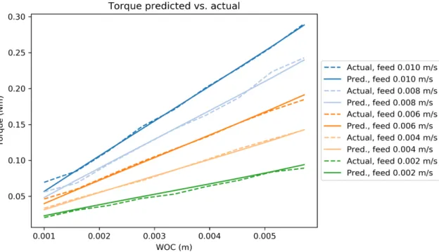
To test the model’s performance in isolation, the machine was directed to take a large number of facing cuts on 6061 aluminum at a variety of feedrates and width-of-cuts. A 0.25" endmill was used with a 1 mm depth-of-cut. Data from these cuts was then used to train the model.

Figures 3-1 and 3-2 show the resulting fit. An 𝑅2 value of 0.987 was achieved with an average prediction error of 3.4%. This is sufficiently accurate for our system.

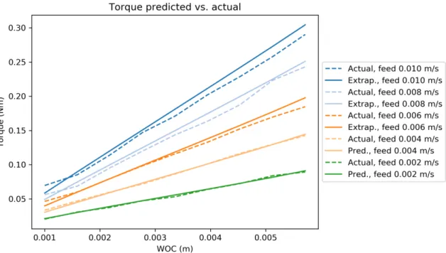
An additional test was performed in which the model was only given feedrates be-low 0.004 m/s and then asked to extrapolate predictions for higher feedrates. Figures 3-3 and 3-4 show that the extrapolated predictions are still reasonably accurate; an 𝑅2 _{value of 0.979 was achieved with an average prediction error of 4.1%.}

3.2

Optimization Performance

To test optimization, the system was given control of the feedrate and width-of-cut for each facing pass. Tests were performed on 6061 aluminum with a 0.25" endmill and a 1.5 mm depth-of-cut. The system was directed to keep deflection below 0.1 mm and failure probabilities below 5%. The initial bootstrap cut had a feedrate of 0.001 m/s and a width-of-cut of 1 mm.

Figure 3-5 shows the system’s predictions for each successive cut. Figure 3-6 shows the system’s predictions after it has been trained with data from every cut. The former figure shows that the system was capable of rapidly converging to the ground truth; the latter shows that the final system collected enough data to accurately model all of the cuts it made.

3.3

System Adaptability

To assess the system’s adaptability, the previous test was repeated with multiple different combinations of material and tooling (see 3.1). The machine used had a

Figure 3-1: Model fit for spindle torques

Figure 3-3: Model fit for spindle torques when asked to extrapolate feeds above 0.004

Figure 3-5: Convergence of model to ground-truth data over successive cuts

maximum feedrate of 0.01 m/s; the depth-of-cut for each run was set such that the optimizer would not reach this limiting feedrate at model convergence.

Material w/ 0.125" w/ 0.25" w/ 0.375"

1018 Low Carbon Steel * _{X X}

304 Stainless Steel _{X X X} 360 Brass _{X X X} 4140 Alloy Steel * _{X X} 6061 Aluminum * _{X X} Polycarbonate Plastic _{X X X} UHMWPE Plastic _X

Table 3.1: Materials tested & endmill diameters used.

All of the material and tool diameter combinations with a _{Xworked as expected;} the system converged on cutting parameters that resulted in a successful cut. Com-binations with a star had some negative aspects that will be discussed.

Tests performed on 304 stainless steel are of notable interest. Despite this mate-rial’s notoriously poor machinability, the system still converged on reasonable cutting parameters for all three endmills.

Tests performed on 1018 steel and 4140 alloy steel with a 0.125" endmill were successful, but their optimization process was somewhat risky. As shown in figure 3-8a, the second cut made resulted in a large spike in torques and forces. This could be attributed to deficiencies in the bootstrapping process.

Tests performed on 6061 aluminum with a 0.125" endmill resulted in tool failure due to chip welding on the 7th facing pass. The system had interestingly converged on the tool manufacturer’s recommended chip load of 0.025 mm before failure occurred. A new test (shown in figure 3-8b) was performed in which isopropyl alcohol was used as mist coolant; no failures occurred. It can be presumed that thermal effects caused the original test to fail.

(a) 360 brass w/ a 0.125" endmill (b) 304 stainless w/ a 0.375" endmill

Figure 3-7: Convergence examples for successful tests

(a) 4140 steel w/ a 0.125" endmill. Note the large spike in forces

(b) 6061 aluminum w/ a 0.125" endmill and mist coolant

Chapter 4

Conclusion

Evaluation of the system proved that it was capable of constructing an accurate model of the milling process with minimal intervention. Further evaluation proved that this model could be used to optimize cutting performance while taking several constraints into account. The system adapted to multiple materials and performed successful cuts even when presented with challenging conditions.

In a larger sense, this system showed that a controller capable of building an internal model of the milling process could have the potential to abstract out much of the hassle associated with milling parameter selection. Intelligent controllers made in this fashion could bring CNC milling closer to being a click-and-watch process and remove human intuition as a prerequisite.

4.1

Future Work

In its current state, the system does not provide a user-ready abstraction for milling arbitrary parts - but with additional work, it is not unimaginable that it could be progressed to that point. Some of the deficiencies in this abstraction can be attributed to unmodeled failure modes while others stem from an unrefined workflow. Once addressed, this system could feasibly be used in a commercial environment.

4.1.1

Modeling Improvements

Evaluation revealed that the system was still susceptible to temperature-based fail-ure modes. Thermal failfail-ures occur when localized heating in either the material or tooling results in undesired material transformations (e.g melting, work-hardening). Localized heating, in turn, typically occurs when chips produced during cutting are not carrying away enough thermal energy.

The flow of heat during milling is governed by complex tribological rules. The amount of work put into the system is well-defined, but the ways in which it dissipates heat are not; a simple model that describes this process would likely need to rely on empirically determined coefficients. As with our cutting force model, a sensor capable of measuring the flow of heat would be needed to find these coefficients. Low-cost LWIR thermal cameras combined with rudimentary image processing could perform this task well.

Evaluation also revealed that the bootstrapping method used was not robust enough to work with all material and endmill combinations. A bootstrapping method that employs Bayesian reasoning might yield more consistent results. Bayesian linear regression, in particular, would allow the model’s predictions to be accompanied by a confidence interval. Predictions drawn from the upper end of this confidence inter-val would be naturally conservative at first. As the model improves, the confidence interval would converge to the mean.

Models to predict machine chatter generally rely on a frequency-response char-acterization of the machine. This charchar-acterization is used to calculate a stability lobe diagram that describes chatter-free machining conditions [16]. A modified ver-sion of this system could attempt to automatically characterize the machine using a solenoid-based impact hammer (as described in [8]).

Alternatively, readings from a high-bandwidth MEMs accelerometer could be used to directly detect chatter during machining. Stability lobe functions are ultimately defined by a small number of coefficients; with enough data, regression could be used to directly infer the final function.

4.1.2

Workflow Improvements

Traditional G-Code-based workflows are not amiable to feedback and rely on pre-computed tool trajectories. Fully employing this system would require an alternate control scheme that allows for real-time trajectory generation and manipulation. An imagined implementation of this new workflow could combine toolpath generation and machine control into a single cooperative unit. As new data becomes available in real-time, internal models could be improved and used to continuously generate updated toolpaths.

Distributed dataflow machine controllers as described by Jake Read [17] are ex-tremely well-suited for this task and would allow this system to be used to its full potential. A dataflow implementation of this controller could be integrated with a real-time toolpath generator. This integrated system could then be utilized on any machine with the appropriate hardware.

4.2

Final Thoughts

It is an outright certainty that manufacturing technology will continue to grow more advanced - we must be careful not to let it outpace our capacity to use it. If we build good abstractions for our machines, we can move closer to a future where personal fabrication is demystified for the masses.

Bibliography

[1] Computer numerical control machines market size, share & trends analysis report by type (milling machines), by end use (automotive, industrial), by region, and segment forecasts, 2020 - 2027. Technical report, Grand View Research, 2020. [2] 3d printing market size, share & trends analysis report by material, by

compo-nent (hardware, services), by printer type (desktop, industrial), by technology, by software, by application, by vertical, and segment forecasts, 2020 - 2027. Technical report, Grand View Research, 2020.

[3] E. Budak. Analytical models for high performance milling. part i: Cutting forces, structural deformations and tolerance integrity. International Journal of Machine Tools and Manufacture, 46(12):1478 – 1488, 2006.

[4] Won-Soo Yun and Dong-Woo Cho. Accurate 3-d cutting force prediction using cutting condition independent coefficients in end milling. International Journal of Machine Tools and Manufacture, 41(4):463 – 478, 2001.

[5] G. Yu cesan and Y. Altintas¸. Prediction of Ball End Milling Forces. Journal of Engineering for Industry, 118(1):95–103, 02 1996.

[6] Mustapha Elhachimi, Serge Torbaty, and Pierre Joyot. Mechanical modelling of high speed drilling. 1: predicting torque and thrust. International Journal of Machine Tools and Manufacture, 39(4):553 – 568, 1999.

[7] Qiaokang Liang, Dan Zhang, Wu Wanneng, and Kunlin Zou. Methods and research for multi-component cutting force sensing devices and approaches in machining. Sensors, 16:1926, 11 2016.

[8] Keith Dunwoody. Automated identification of cutting force coefficients and tool dynamics on cnc machines. 01 2010.

[9] Dohyun Kim and Doyoung Jeon. Fuzzy-logic control of cutting forces in cnc milling processes using motor currents as indirect force sensors. Precision Engi-neering, 35(1):143 – 152, 2011.

[10] J.A. Nemes, S. Asamoah-Attiah, E. Budak, and L. Kops. Cutting load capacity of end mills with complex geometry. CIRP Annals, 50(1):65 – 68, 2001.

[11] Lucjan Kops and D. T. Vo. Determination of the equivalent diameter of an end mill based on its compliance. 1990.

[12] E.B. Kivanc and E. Budak. Structural modeling of end mills for form error and stability analysis. International Journal of Machine Tools and Manufacture, 44(11):1151 – 1161, 2004.

[13] U. Zuperl, F. Cus, and M. Milfelner. Fuzzy control strategy for an adaptive force control in end-milling. Journal of Materials Processing Technology, 164-165:1472 – 1478, 2005. AMPT/AMME05 Part 2.

[14] U. Zuperl, F. Cus, and M. Reibenschuh. Neural control strategy of constant cutting force system in end milling. Robotics and Computer-Integrated Manufac-turing, 27(3):485 – 493, 2011.

[15] L. Kops and D.T. Vo. Determination of the equivalent diameter of an end mill based on its compliance. CIRP Annals, 39(1):93 – 96, 1990.

[16] Jianping Yue. Creating a stability lobe diagram. pages 301–50, 01 2006.

[17] Jake R Read. Distributed dataflow machine controllers. Master’s thesis, Center for Bits and Atoms, Feb 2020.