BAROCLINIC VORTICES OVER A SLOPING
BOTTOM
by
Joseph H. LaCasce, Jr.
A.B., Bowdoin College, 1986 M.S., Johns Hopkins University, 1988 Submitted in partial fulfillment of the
requirements for the degree of Doctor of Philosophy
at the
MASSACHUSETTS INSTITUTE OF TECHNOLOGY and the
WOODS HOLE OCEANOGRAPHIC INSTITUTION September 1996
@ Joseph H. LaCasce Jr. 1996 All rights reserved The author hereby grants to MIT
and to distribute copies of this
Signature of Author...
Certified by ....
and to WHOI permission to reproduce thesis document in whole or in part.
. . ... .. . .. . .. .. . .. . .. . .. .. Joint Program in Physical Oceanography
Massachusetts Institute of Technology Woods Hole Oceanographic Institution August 23, 1996
. . .. .. . .. .. .. . . . . . ... Dr. Kenneth H. Brink Senior Scientist, W.H.O.I.
Thesis Supervisor
Accepted by ... ... ... ...- -
---Professor Paola Malanotte-Rizzoli Ch ai fi7 0mmittee for Physical Oceanography
a, Massachusetts Institute of Technology
Woods Hole Oceanographic Institution
BAROCLINIC VORTICES OVER A SLOPING BOTTOM by
Joseph H. LaCasce, Jr.
Submitted in partial fulfillment of the requirements for the degree of Doctor of Philosophy at the Massachusetts Institute of Technology
and the Woods Hole Oceanographic Institution August 23, 1996
Abstract
Nonlinear quasigeostrophic flows in two layers over a topographic slope are considered. Scaling the lower layer potential vorticity equation yields two pa-rameters which indicate the degree of nonlinearity in the lower layer. The first,
u' (the strength of the deep flow divided by the product of the effective bottom slope and the squared length scale), is related to the advection of relative vortic-ity, and the second, fU 1 (the product of the inverse square deformation radius
of the lower layer and the strength of the surface flow divided by the effective slope), to the advection of vorticity due to interfacial stretching.
Two types of isolated vortex are used to examine the parameter dependence. An initially barotropic vortex remains barotropic only when f3-2 > 1; otherwise
2L 2
topographic waves are favored at depth, and the vortex separates into a surface vortex and waves. In the latter case, the surface vortex is weakened, consistent with a simple linear theory. An initially surface-trapped vortex which is larger than deformation scale is baroclinically unstable when 9 > 1. If , < 1, radiation of disturbances hinders or even blocks unstable growth, permitting the existence of large, stable surface vortices.
Both parameters are also relevant to cascading geostrophic turbulence over a slope. If F2U1 > 1, a "barotropic cascade" occurs at the deformation radius (Rhines, 1977) and the cascade is arrested at the scale at which =_ 011 O . The resulting flow is dominated by large scale, anisotropic topographic waves. If < 1, layer coupling is hindered and the cascade is arrested at the deformation scale. The flow then is dominated by isotropic surface vortices which continually
"leak" energy to topographic waves at a rate proportional to A.
In both single vortex and turbulence cases, the distinction between vortices and waves is more transparent when viewing potential vorticity. It is more dif-ficult to identify waves and vortices from the streamfunction fields, because the waves are present in both layers.
Thesis Supervisor: Kenneth H. Brink
Senior Scientist, Department of Physical Oceanography Woods Hole Oceanographic Institution
~----L---.-~-_~r;_r^_---_~-Acknowledgements
I am grateful to Ken Brink for much good advice, patience and many inter-esting conversations. I am also indebted to committee members Dave Chapman, Glenn Flierl, Joe Pedlosky and Steve Lentz for numerous thought-provoking sug-gestions which greatly improved the work. Glenn's numerical model worked like a well-oiled machine, which freed up time for thinking about the dynamics. Paola Rizzoli was a delightful chairperson for the defense, and cheerfully agreed to sign a wicker blind when I told her that the Institution was out of archival bond.
Many people allowed me to moonlight on their computers for my calculations, which was tremendously beneficial to the work. Linda Meinke and Charmaine King were wonderful, and forgiving of exceeded quotas. Terry Joyce let me use the WOCE computer, which was much faster than my previous machines, and Jane Dunworth was always cheerful and helpful when there were problems. Higher resolution required even faster machines. Edmund Chang at MIT let me use his alpha to do some of the 2562 grid point calculations, and Mike Spall lent his Silicon graphics machine for a blissful month while he was in Florida; many of the single vortex runs were calculated then. Audrey Rogerson has the same machine, and let me do many calculations, including the "strong slope run" which took 6 days. Audrey also introduced me to the numerical filter used in all of the runs in this thesis. Finally, Jamie Pringle kept me out of trouble by allowing me to store data on a disc he set up.
I have been fortunate to have many good and interesting friends while in the department who helped make my time here so enjoyable; in fact, I might have finished faster if I hadn't been so content here. When we arrived at the generals, there were two of us, and my only classmate, Young-gyu Park, has been a constant friend and great resource. Bruce Warren has also been a close friend with whom I've enjoyed many chats on topics ranging from the ACC to the best Boris Gudonov. I've had frequent talks with many students in the department which were often enlightening, and only once came down to a bet for beer. Barbara Gaffron always guided me when I was lost, and has also been a good friend.
In terms of distractions, I've spent much time (and even lived with) a group of close friends who were able to maintain what I considered to be a "healthy" lifestyle, despite work requirements. Even if the water wasn't actually "boiling" with bluefish, we always had a superb time waiting. Thanks also to the group of regulars who kept the Journal Club afloat and the discussions lively, even when the articles were, well, less so. The movie club (president, Birgit Klein) also suffered through several less inspired pieces, and had fun doing it. The soccer players (president, Debbie Smith) were always ready for a game, even when it looked like sleet was inevitable. And participating in the present incarnation of
the Woods Hole chamber music society has been great fun.
Finally, thanks to my two families. Cecilie Mauritzen is not only a dear wife, but she is a good and critical audience for ideas about oceanography. Johannes is a delight; he had lots to say about the thesis, though I couldn't understand most of it. Its been wonderful being so near my other family for the last few years as well: my parents and my two sisters. They have always been supportive and loving, for which I am very grateful.
Funding for this research was provided by Office of Naval Research Coastal Science Code, grants N00014-92-J-1643 and N00014-92-J-1528.
Contents
Abstract 3 Acknowledgements 5 1 Introduction 9 1.1 Previous work ... ... 12 1.2 Thesis approach ... 17 2 Model 19 2.1 Equations . . . 19 2.2 Scalings . . . 22 2.3 Numerical method ... 24 2.4 Sponge ... . . . . ... . ... ... ... . 26 2.5 Damping ... ... . ... 27 2.6 Vortex counting ... 332.7 Quadratic Invariants and Spectral Fluxes . ... 34
3 A single vortex over a slope 40 3.1 Initial conditions .. .. .. ... .. .. .. .. ... .. .. .. . 41
3.2 One layer results ... 43
3.3 Two-layer results: A barotropic vortex . ... 53
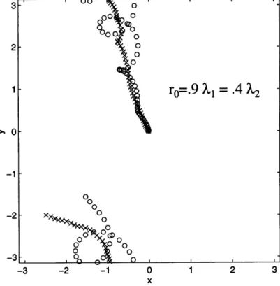
3.3.1 Case A: r = 2.5A, 2 = .02 ... 53
3.3.2 Case B: ro = .64A, 82 = .02 ... 59
3.3.3 Case C: ro = .64A, 82 = 36 .... ... . 69
3.3.4 Intermediate slopes with ro = .64A . ... 79
3.3.5 Case D: r = 2.5A, 82= 36 ... 81
3.3.6 Intermediate slopes with ro = 2.5A . ... 86
3.4 Two-layer results: A surface vortex . ... 93
3.5 D iscussion . . . . . . . .. 108
Appendix A: Non-isolated Vortex ... 114
4 Geostrophic turbulence over a slope
4.1 Background: Barotropic turbulence . . . . 4.2 Initial conditions ...
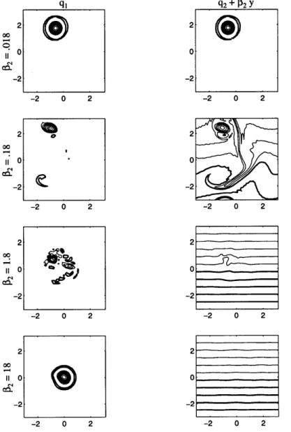
4.3 Weak slope: A = 4 ...
4.3.1 Streamfunction and energy ...
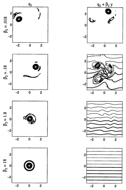
4.3.2 Potential vorticity and surface vortices . . 4.4 Strong slope: A = .1 ...
4.4.1 Streamfunction and energy . . . . 4.4.2 Potential vorticity and surface vortices . . 4.5 Discussion . . . . .. . . .. . . . .. . . .. .. . 4.5.1 Arrest: the Rhines diagram . . . . 4.5.2 Vortices . .. . . .. . . . .. . . . . 4.5.3 Potential vorticity: the RMS PV diagram 4.5.4 Observations ... 130 . . . . .131 . . . 135 . . . 138 . . . 138 . . . . .146 . . . 159 . . . . .160 . . . 170 . . . 181 . . . . . 181 . . . 186 . . . 187 . . . 190
Appendix B: Geostrophic turbulence with a bottom Ekman layer 5 Conclusions 5.1 Continuous Stratification . . . . 5.2 PlanetaryP . ... 5.3 Modifications and Future Work ... References . . . 193 199 . . .202 ... 204 ... 208 212
Chapter 1
Introduction
The variation of the Coriolis parameter with latitude, the so-called p-effect, has a profound effect on oceanic flows. In particular, the variation produces a restor-ing force which opposes meridional motion and therefore supports Rossby waves. These waves are dispersive, and the phase speed is always westward. This west-ward orientation has been linked to the western intensification of the wind-forced currents in the ocean, i.e. the reason the Gulf Stream lies off the eastern coast of North America rather than the western coast of Europe. It is also known that larger scale motion "feels" the ,-effect more than does small scale motion, a fact which makes the larger scales more wave-like but permits nonlinearity at smaller scales (Rhines, 1975).
In a barotropic fluid, topography acts in an analogous manner, i.e. it yields a restoring force which opposes cross-isobath motion. However, the orientation of this "topographic fl-effect" can change, so that the "westward" propagation of the waves relative to the topography could in fact be in any direction. Secondly, the strength of the topography can vary, and in many cases can greatly exceed the planetary P. A stronger P favors linear motion at smaller and smaller scales, leading to an expectation of predominantly wave-like motion over steep slopes.
With the introduction of stratification, the problem changes considerably. In ,.---rrr. rYYY~III~LII -.- ~I__L-CI~^I.I_ ..-. .-LX-_I~-- Llllllfl~ ~L1 LIIII3~~
particular, stratification can "shield" flow at the surface from the effects of the topography, perhaps negating its influence. Put another way, if a flow does not advect fluid across the topography, it cannot generate waves and therefore does not interact with the topography. This suggests that a steep slope no longer necessitates wave-like flow, because flow at the surface may be nonlinear. Unlike the planetary 3-effect, the effect of topography in a stratified fluid varies in the vertical. This vertical asymmetry of the topographic P can yield interesting results.
As an example, consider a system in which the stratification is approximated by two immiscible layers. In the planetary # case, a meridional restoring force exists in both layers. One says that such motion induces changes in perturbation potential vorticity (PV) in both layers. Two types of Rossby wave are supported: one with parallel particle meridional displacements in each layer (the barotropic mode), and another with anti-parallel motion (the baroclinic mode). Any initial disturbance can be broken into these two types of waves.
In contrast, and as noted above, only motion across the slope in the lower layer is opposed by the topographic
/
(if one assumes the planetary gradient is zero); motion in any direction at the surface is unopposed, i.e. causes no change in PV. A result is that topographic waves have only one propagating mode. This mode actually has particle displacements in each layer which are parallel, but the amplitude of the surface displacements is always smaller than at depth, and more so for small-scale waves (which are bottom-trapped) (Rhines, 1970). An initial value problem on the topographic3
plane thus has a very different outcome: a portion of the disturbance propagates away, but a portion may be left behind.This fact has profound effects in what follows.
A similar comparison is between a two-layer system in which Ekman damping acts in both layers and another in which it only acts at the bottom. In particular, consider the effects on a (baroclinically) unstable flow. In the symmetric damping
case, damping inhibits the growth of disturbances, i.e. it stabilizes the flow (Pedlosky, 1987). In the asymmetric case the dissipation actually destabilizes the flow, so that the small disturbances grow before eventually decaying, leaving the original flow altered (Pedlosky, 1983). Anticipating the latter result given only the outcome of the symmetrically damped case would be difficult.
There are numerous examples of strong surface flows adjacent to or over strong topography in the ocean. Rings which pinch off from the Gulf stream are known to migrate back towards the continental slope, and cross severe to-pographic features (Joyce, 1983; Cheney and Richardson, 1976). Likewise, the large Agulhas Eddies which migrate across the South Atlantic must pass over severe ridges, and are occasionally blocked there (van Ballegooyen et al., 1994). The California Current is an intense Eastern boundary current which lies adja-cent to the continental slope and spawns eddies which may even move on to the shelf nearby (Largier et al., 1993). With the large number of unstable boundary currents in the ocean, interactions between intense eddies and strong topography are expected to be common.
The present work seeks to characterize the evolution of such eddies in the presence of stratification and bottom topography. In addition, I examine how flows which are familiar on the /-plane are altered on the topographic O-plane. Two specific cases are considered: a single vortex and a turbulent flow (multiple vortices). As explained below, there are numerous studies of both flows with the planetary 8, but much less is known about how they evolve over topography.
The specific questions addressed are: 1) under what conditions do the sym-metric and asymsym-metric p cases agree? 2) in cases in which they don't agree, how does one characterize the evolution and, in particular, the baroclinicity of the resulting flow? The more specific questions focus on whether an eddy can move across topography, perhaps from offshore into shallower water, or how cascading turbulence "arrests" over a slope.
1.1
Previous work
The single vortex over a slope has been studied previously primarily as a model for large oceanic rings. However, the barotropic case with P has been even more widely examined as a model for self-induced hurricane motion. A linear vortex of either sign drifts westward (Flierl 1977) and disperses rapidly, suggesting that meridional motion and the observed longevity of rings (of order several years, e.g. Cheney and Richardson, 1976) are likely the results of nonlinearity. McWilliams and Flierl (1979) found that a strongly nonlinear vortex decayed at a slower rate, and found a meridional component of translation velocity. The latter was first postulated by Rossby (1948) who noted that a vortex causes a deflection of the mean PV field and thus will tend to migrate meridionally to reduce this deflection. Adem (1956) showed by means of a Taylor expansion in time that a cyclonic vortex drifts initially to the northwest.
Subsequent work (e.g. Chan and Williams, 1987; Fiorini and Elsberry, 1991; Resnik and Dewar, 1995) has sought to explain the self-induced motion in the strongly nonlinear limit, and to predict the initial velocity. The mechanism (now widely accepted) is related to the development of asymmetries in the vortex shape; as fluid on the sides of the vortex is advected meridionally, it acquires relative vorticity. A negative vorticity anomaly develops to the east of a cyclone, and a symmetric positive anomaly to its west, making the positive vortex appear stretched to the west and compressed to the east. The (dipolar) anomaly field can advect the primary vortex and the whole system will translate; by the signs of the anomalies, one deduces that a cyclone moves northward, and an anti-cyclone southward. Rossby waves are generally found in the wake, indicating decay and dispersal of the eddy.
Warren (1967) was apparently the first to note that similar self-induced mo-tion could occur over topography. In agreement with this, Carnevale et al. (1991)
found that a cyclonic vortex moves to the local "northwest", or towards shallower water and to the left (facing shallower water), over a variety of sloping bottoms in the laboratory. Others have then sought to understand the specific influence of the continental slope on barotropic rings. Wang (1992) considered such a case with a hierarchy of models, and Grimshaw et al. (1994) approached the problem with the shallow water equations.
Others have considered stratified vortices on a P-plane, often with either an infinitely deep lower layer or a flat bottom, e.g. McWilliams and Flierl (1979), Mied and Lindemann (1979) and McWilliams and Gent (1986). All find a north-westward/southwestward drift for cyclones/anti-cyclones. However, the addition of baroclinicity can alter the dynamics. The elimination of the barotropic mode (in the deep lower layer or the one and a half layer case) appears to significantly reduce the speed of translation. In the flat bottom case, the vortex may evolve to a baroclinic dipole (e.g. Flierl et al., 1980) with an eastward velocity, though this typically occurred with an initial vortex with no barotropic component. For the more general initial vortex with some barotropic flow, the evolution closely resembled that of the one layer experiments.
Previous baroclinic eddy studies over topography fall into two categories. In the first, the eddy is bottom-trapped on a slope beneath an infinitely deep upper layer, often as a blob of dense fluid. The theoretical studies of Nof (1983) and Killworth (1984) are examples, as are the laboratory studies of Mory et al. (1987) and Whitehead et al. (1990). Nof (1983) argued that the (cyclonic) vortex would drift westward under the influence of gravity and predicted a velocity consistent with that observed in Whitehead et al. (1990). Interestingly, Mory et al. (1987) found a northwestward drift with their cyclonic vortex, much more like the Carnevale et al. (1991) vortex (see Chapter 3 for more discussion of the discrepancy.)
In the second category, the eddy is usually surface-intensified. Smith and ~~~_I_____I__ IILXIU* _m^YI .-)I~YII~Y~-*YLYI~Y
O'Brien (1983), following on initial numerical work by Haustein (1981), studied a two-layer ring impacting a strong linear slope using a primitive equation model. They suggested that the effects of the planetary and topographic P effects would be additive (as one might expect in a barotropic fluid). They found that a vortex with zero initial deep flow was not affected by the slope. In a similar vein, Kamenkovich et al. (1995), in a two layer, primitive equation study, noted the degree of interaction between a steep ridge and an Agulhas eddy depended on how barotropic the vortex was, but that the vortex became "compensated" (zero deep flow) after hitting the ridge. Strongly barotropic vortices could stall over the ridge, as they are sometimes observed to do in the South Atlantic.
In relation to the continental shelf, the important question is whether offshore eddies can influence currents over the continental slope and shelf. Washburn et al. (1993) examined an anticyclone that essentially hovered over the Northern Cal-ifornia shelf for two months, transporting suspended sediment offshore. Largier et al. (1993) found that a significant portion of the current variability there was due to offshore eddies. In terms of modelling, Chapman and Brink (1987) found in the linear case that offshore forcing of shelf currents was greatest when coastal trapped waves were excited. Qiu (1990) found that the addition of planetary ,
allowed for surface wave motion which in turn could induce surface variability over the shelf.
A closely related area of study has focussed on intense topographic waves over the Continental slope, e.g. the slope off the east coast of the U.S. (Thompson and Luyten, 1976). Hogg (1981), Welsh et al. (1991) and Pickart (1995) have found evidence linking the waves with Gulf Stream meanders. Louis and Smith
(1982), Shaw and Divakar (1987) and others have suggested that the waves may be generated by rings impacting the slope. A detailed review is given in Smith
(1983).
Thus significant work has been done on single eddies over topography, both
in the linear and nonlinear limits. Fewer results exist for more complicated nonlinear flows over topography. However, there is a large body of literature on two dimensional or "geostrophic" turbulence, both with and without a P effect.
In contrast to three dimensional turbulence in which energy is transferred to small scales where it is dissipated by viscous processes, energy in two-dimensions is transferred to large scales. The possibility of such an inverse cascade of energy was apparently first postulated by Onsager (1949) and Fjortoft (1953). Simul-taneous with the energy cascade is a forward cascade (towards small scales) of enstrophy (squared vorticity), which is also dissipated by viscous action. Spec-tral aspects of both cascades (in particular the details of the cascading inertial subranges for enstrophy and energy) were postulated by Kraichnan (1967, 1971) and Batchelor (1969). Recent work on the subject has focussed on the effects of intermittency, in the form of coherent vortices; Basdevant et al. (1981) showed that intermittency led to a steepening of spectra in the enstrophy inertial range, McWilliams (1984, 1990) demonstrated that coherent vortices dominate the dy-namics of freely evolving turbulence at later lates and Babiano et al. (1987) illustrated the importance of vortices in forced-dissipative turbulence.
Related research has focussed on how various imposed effects could alter the barotropic cascade. Rhines (1975) found that the p-effect led to an arrest of the inverse cascade, at a scale at which Rossby wave processes dominate advective processes, as waves are much less efficient at transferring energy. His numerical simulations moreover suggested the formation of zonally-oriented jets. Holloway (1978) and Herring (1977) found that small-scale bottom bumps could cause a flux of energy toward the scale of the topography, via nonlinear (triad) inter-actions. They also found a stationary, topographically-locked component of the flow, predicted as a state of "minimum enstrophy" (Bretherton and Haidvogel, 1976) or maximum entropy (Holloway, 1978). Shepherd (1987) found that the presence of a large scale zonal jet (as in the atmosphere) affected the arrest of
energy both by altering the effective # and by direct shearing of the vorticity field by the jet.
The other significant complication which has been explored is stratification. Charney (1971) showed that under the quasigeostrophic approximation and the assumption of homogeneity, the conservation of potential vorticity guaranteed an inverse cascade to larger horizontal and vertical scales. He also suggested that enstrophy in such a case be replaced by potential enstrophy, or squared potential vorticity, but that otherwise the 2-D formalism carried over. Rhines (1977) suggested, along similar lines, that small-scale baroclinic energy in a two-layer flow would undergo a "barotropic cascade" upon reaching the deformation radius. Thereafter, the cascade to larger scales was essentially as in the one layer case. Noting that wind forcing of the ocean is generally baroclinic and at large scales, Salmon (1980) showed that the initial baroclinic cascade of energy was actually forward, but that the late evolution corresponded to that of Rhines (1977). From the vortex point of view, McWilliams (1990b) has suggested that the barotropic cascade occurs as coherent vortices at different depths align (e.g. Polvani, 1994) to make barotropic vortices.
The problem of stratified turbulence over topography can be seen as a com-bination of two lines of study, i.e. stratified turbulence and topographic effects. Consistent with this, most previous work on the subject has focussed on the effect of bumps on stratified flows, either in layered systems or continuously stratified representations with truncated vertical modes. Rhines (1977) found that bottom bumps inhibited the barotropic cascade of baroclinic energy; however, he also found that the degree of barotropy depended on the initial vertical structure of the flow. Treguier and Hua (1987) found barotropy was achieved when the tur-bulence was forced at the surface, but that the bumps yield smaller horizontal scales than would be found over a flat bottom. Treguier and McWilliams (1990) also observed barotropic small scales, and suggested a link to the stationary
---_IIIYII_-YLiI~-LIYtllllllllllW-graphic mode discussed by Herring (1977). Vallis and Maltrud (1994) considered other types of topography, and found jet formation to occur over a ridge, as well as the development of a temporal mean "westward" component of the flow. The latter they linked to the stationary topographic mode, and the former to the jets observed on the -plane by Rhines (1975).
1.2
Thesis approach
The examples considered hereafter are quite similar to the stratified topographic cases above: I examine a two-layer single vortex over a slope, as did Smith and O'Brien (1983) and Kamenkovich et al. (1995), and two-layer turbulence over a slope like Vallis and Maltrud (1994). But while the examples are similar, the approach is somewhat different. In particular, I restrict attention to the f-plane over a slope so that the only waves present are topographic waves. This permits a clearer picture of evolution by allowing for a separation into waves and "vortices", in most cases, and also aids the comparison to the purely barotropic case. Moreover, I will employ a quasigeostrophic model, rather than the primitive equations.
The specific approach is to examine numerical initial-value problems in two-layer flows, with an idealized slope (a linear gradient). Under quasigeostrophy the flow is assumed to be geostrophic at lowest order (Pedlosky, 1987); specific restrictions are discussed in the model section, Chapter 2. Quasigeostrophy is adopted essentially for practical reasons: the simplified calculations permit a more thorough examination of parameter space than would a primitive equa-tion study. The two-layer approximaequa-tion similarly shortens computaequa-tions, but also the simpler vertical structure is easier to interpret. One nevertheless finds considerable complexity, even with this simplified system.
In addition to the general object of characterizing the differences obtained by
~I ^--. I---.-i- -~-. ~- -~11~ --- 1 -~Ill--~-^-I IYLIPY-~IILYL -LIIY~ L__ ( LillBI
introducing baroclincity to the problem, there are also several additional specific goals. As the single vortex case has relevance to the motion of oceanic rings, the self-induced translation of the vortex over the slope with varying stratification and slope is quantified. The baroclinic stability of the vortex is also of great importance, for ocean rings and for interpreting the results of the more general, turbulent case. In the latter case, the arrest of the inverse cascade is sought under varying stratification and steepness of the slope.
The equations and model used for the numerical runs are described in Chap-ter 2. Scalings of the two-layer equations are discussed, as are particulars about the numerical implementation. Chapter 3 reviews the case of an isolated single vortex on the 3-plane, then discusses the fate of an initially barotropic vortex and a surface vortex over the slope. An appendix (A) is included which discuss the related case of a non-isolated vortex. In Chapter 4, turbulence over a slope discussed, with comparisons to the better known two-layer case with a flat bot-tom, as well as to the case with an infinitely deep lower layer. An appendix (B) follows which presents results from a another asymmetric case, one with only a bottom Ekman layer (no bottom slope). Chapter 5 concludes the work, and discusses the results in light of previous findings, as well as highlights specific shortcomings.
Chapter 2
Model
The equations which were used are presented below and several nondimensional parameters are found by scaling these equations. The spectral model used for the calculations is also explained, with some discussion of resolution issues and of the damping ("sponging") of waves. Unlike many contemporary numerical studies,
a numerical filter is used rather than so-called "hyperviscosity", and the benefits (and drawbacks) of the filter are discussed in the final section.
2.1
Equations
The model is one of the simplest which incorporates advection, stratification and topography: a two-layer, quasigeostrophic model with a linearly sloping bottom. The quasigeostrophic (QG) limit implies a small Rossby number, small interface displacements and weak topographic slopes (Pedlosky, 1987) and thus is not strictly valid for oceanic regions with fronts and/or large bottom slopes. This will be discussed more below.
The relative simplicity of quasigeostrophy makes analytical solutions more tractable, and permits higher horizontal resolution in numerical experiments, compared to comparable primitive equation models. Higher resolution allows for
a reduction of lateral damping effects and is thus desirable in simulations of invis-cid fluids. An additional numerical benefit of QG is that the vorticity equations are advanced in time rather than the momentum equations. This in turn allows the inclusion of a mean PV gradient, such as due to the 3 effect or a slope, in a periodic domain, i.e. one without lateral boundaries and boundary layers. In the case of homogeneous turbulence, this is a considerable simplification.
The inviscid, dimensional equations for the layer potential vorticities in the case of topography which only varies in the y direction are (e.g. Pedlosky 1987):
a
qx + J(bl, 1) = 0 (2.1) 8 8a
q2 + J(02, q2) + 2a 2 = 0 (2.2) with qj - V 2 2 + Fi(3-i - Ok) the "perturbation potential vorticity" and 0j
the streamfunction for layers i=1,2 with V2 the horizontal (two dimensional)
Laplacian operator. The (squared) inverse of the deformation radius in each
layer is F = -f2 with g' = P2 Pg the reduced gravity (pi is the density in layer i, po a reference density, and g the acceleration due to gravity), f the Coriolis parameter, and Hi the depth of the layer. The Jacobian is defined as J(a, b) ( - a). Here qi is conserved on fluid parcels, but q2 is not, but changes as the parcels move across isobaths. Rather the "total potential vorticity" in layer two (q2 + 02 y) is conserved on parcels.
One can define F2 - 6F where 6 - H is the ratio of layer depths. In theH2 ocean, 6 might be the ratio of the depth of water above the thermocline to that below, and, if so, has a typical value of about 0.2. The ratio is generally assumed
to be unity in the numerical runs for simplicity, but I will retain unequal layer depths in the expressions discussed hereafter for generality.
The slope is taken to be linear and shallowing in y, so that P2 - (OH 2)
Note that on the f-plane, there is no loss of generality in orienting the slope in this direction. The expression for p2 can be found in a manner analagous to the one layer case, where the full PV is given by:
q 2v0 + f (2.3) h
where e = is the Rossby number, assumed small. If h = h - a __hnd
=-OIe| (L being the horizontal scale of motion), the PV can be rewritten:
1 2fh
q 2 +f y) (2.4)
The definition of
pa
given above then follows. Note that the expansion is carried out in the lower layer in the two layer case, so that h is replaced by H2. ThePV gradient in layer two resembles the traditional p-effect and so is called the "topographic
P"
(Faller and VonArx, 1955). The small slope requirement is that the variation in depth is no greater than H; assuming a Rossby number of order .1, a lower layer depth of 1 km and a scale of motion of 10 km yields a maximum grade of about 1%, a not unreasonably small number. However, QG is often avoided precisely for this limitation. Results presented later on will show that the effects of the slope can be large, even within QG.In previous studies, both planetary and topographic gradients were included (Smith and O'Brien, 1983; Kamenkovich et al.,1995). Wang (1992) contrasted results obtained on the barotropic f-plane with those found on the a-plane with
topography. The planetary
f
is nevertheless neglected here because its inclusion obscures the interaction with the topography. Expected modifications due to the planetary 6-effect are discussed in Chapter 5.2.2
Scalings
The equations are scaled assuming motion with velocity scales U and U2 and a length scale L, and time scales Ti and T2 (subscript denoting layer). In the upper layer, an advective time scale is appropriate since the surface PV at a given location can only change under the influence of advection. Thus in layer one, Ti a -L. In the lower layer, cross-slope motion also leads to temporal changes in PV, so one may choose an advective time scale or a time scale proportional to the period of the bottom waves. Many of the cases of interest below have little or no bottom flow, so the second choice is more desirable, i.e. T2 a -. Hence there are possibly different time scales in each layer. The difference is due to the vertical asymmetry of the PV gradient, and will be found to have profound effects.
Scaling the potential vorticities in each layer, one finds that the measure of the relative importance of stretching and relative vorticity is determined by:
FIL2 , F
2L2. (2.5)
These terms are the squared ratio of the scale of motion to the internal radius of deformation in each layer. As mentioned, in most of the numerical examples the layer depths are equal, and so there is only one parameter. In the flat-bottom case, the size of the parameters generally indicates the degree of layer coupling.
Scaling the bottom PV equation, (2.2), yields two parameters:
U2 (2.6)
#
2L
2 andF2U
8F
U1 f U (27)/2 02 g'( VH2)
The first parameter is the ratio of PV changes due to the advection of relative vorticity and waves. Equivalently, it compares the deep advective time scale to the topographic wave phase speed, or the ratio of particle to wave speeds. It is the slope analog of the barotropic parameter, discussed by, among others, Rhines (1975). In the barotropic case, the size of the parameter indicates the relative importance of advection and waves to changes in the Eulerian PV. Alternately, it indicates how "strong" the planetary restoring force is for given particle velocities. Similarly, the slope parameter indicates the effective severity of the slope. Note that it depends not only on the slope but the size and strength of the motion, i.e. a larger/weaker vortex "sees" a larger slope than a smaller/stronger vortex.
The second parameter is the ratio of PV changes due to the advection of thickness and waves. The ratio of the first parameter in (2.6) and that in (2.7) is _, 2 and is small when there are large scales of motion and/or when the
deep flow is weak. The thickness parameter is found to be central to baroclinic instability, and thus important in both single and multiple vortex cases.
If both advective parameters are small, the contours of total PV in the lower layer are "open" since they are dominated by the slope contribution. As seen in Chapters 3, the degree of openness of the PV contours in the barotropic, /-plane case indicates how linear the evolution is. Likewise, when the contours are open in the two-layer case, one finds the deep evolution to be more wavelike, and the surface flow to be more baroclinically stable.
2.3
Numerical method
The PV equations in (2.1-2.2) were stepped forward in time with a Fortran code written by Glenn Flierl. Equations (2.1-2.2)were solved spectrally on a doubly-periodic domain (e.g. Canuto et al., 1988), so that all variables are Fourier decomposed in both directions:
1
NN= U E (q, ui) exp(ikx + ily) (2.8)
where N, and N, are the number of grid points (real space). As such, the model has no boundaries, so the region of ocean represented is far from coasts. Moreover, the double periodicity implies that energy which exits one side of the domain enters the opposite side, so waves generated in the domain can re-enter and interact with the original flow. This aspect is perhaps the largest drawback of the model, and is discussed below. The length scale is chosen so that the domain dimensions are 27r by 27r, a common choice which results in integral wavenumbers in spectral space. Variables are alternately referred to by their Fourier and real representations, so the hat distinguishes the Fourier transform (as in (2.8)).
The single vortex runs required fewer grid points than the turbulence runs, as the latter often had of order one hundred vortices. In most cases with the single vortex, using 642 and 1282 grid points (with maximum wavenumbers 32 and 64) yielded quantitatively similar and qualitatively identical results. The model runs were rapid with 642, so that resolution was used most often. In one region of parameter space however, the vortex broke up into smaller vortices, and 1282 points were required. Of course, the required resolution depends on the choice of initial conditions because a smaller initial vortex requires more grid points. But
the vortex used here filled a large portion of the domain, so that there were of order 20 grid points across the diameter of the vortex with 642 points.
The turbulence cases on the other hand required greater resolution. The amount required depended on the initial conditions, but it was desirable to have initial flow with relatively small scales (to yield a larger population of vortices-see for example Santangelo et al., 1989) so more grid points were required. There-fore, the primary runs were made with 2562 grid points. Though this is modest resolution in comparison to recent barotropic calculations (10242 in Santangelo et al., 1989), higher resolution was not feasible given the computer resources available, and the fact that fast waves required a small time step. Many addi-tional runs were made with 1282 points and the qualitative aspects were generally reproduced. Additional details on resolution are presented in Chapter 4.
The model was advanced in time with a standard leap-frog scheme, with an Euler step applied periodically to stabilize the computational mode (e.g. McWilliams, 1990). More sophisticated routines might be required for more quantitative representations of observed flows, but this technique was judged sufficient for the results sought here.
Spectral dealiasing, a technique which removes contributions to the Jacobian from unresolved wavenumbers (Patterson and Orszag, 1971), was also employed. However, the results were nearly identical with and without dealiasing, so long as the resolution was fine enough. The single vortex runs were negligibly altered by de-aliassing (differences in the calculated position of the center of the vortex for a typical set of parameters were in the fourth decimal place), but turbulence runs with 1282 grid points benefited somewhat (dissipation was decreased by a few percent). The higher resolution turbulence runs were not significantly improved. As dealiassing lengthened the computational time by roughly 50%, it was not used.
~u~-~-~-2.4
Sponge
As mentioned, a drawback of double periodicity is that waves may exit one side of the domain and re-enter the other side, leading to multiple interactions with the primary flows (vortices). Often the interaction was weak enough to ignore, but in some cases the primary flow was severely distorted by the waves. In the single vortex cases, the problem was remedied with a "sponge" layer, of the following form:
sponge = .5 + .25 * (tanh((x - .3)/10) + tanh((27r - x + .3)/10)) (2.9)
This function, which is basically unity over most of the domain but decays to .5 in a boundary layer of half-width .3 at the left and right edges of the domain, multiplied the perturbation potential vorticity in the lower layer (for reasons discussed below) at each time step. The sponge only decays to .5 because the vortex was found to excite domain-scale normal modes with more severe filters. The sponge was more successful with smaller scale waves, which had a strong signature in vorticity, than with larger scale waves. In most cases, the sponge sufficiently weakened the re-entrant waves, but in one case more drastic measures were required, as discussed in Chapter 3.
A sponge was not used with the turbulence runs. By removing vorticity at the edges of the domain, the sponge catalyzed the rapid formation of zonal jets, i.e. structures with no zonal gradient of vorticity. As mentioned in Chapter 4, using a bottom Ekman layer is one way to damp the waves, but the Ekman layer itself changes the stability properties of the surface flow (Pedlosky, 1983). Therefore, the base runs were made with no Ekman damping. However, additional runs
were made in which layer decoupling was accomplished solely by a bottom Ekman layer, for comparison. The details are given in Appendix B.
2.5
Damping
When the inviscid potential vorticity equations (2.1-2.2) are advanced in time, numerical instability often results as energy accumulates at the smallest scales. This is usually avoided by including a diffusion term on the right hand side of the equations, as a model for unresolved small scale dissipative processes. Common
forms are a Laplacian diffusion, 2 2 qi, or a "bi-harmonic" diffusion, v4 V4 q (e.g. McWilliams 1984), although higher order schemes are often used. Generally vi is adjusted to minimize viscous damping of the flow and, with sufficient numerical resolution, the effects on the larger scale dynamics usually are generally small. However, there are negative aspects. Diffusion causes decay, albeit slow, of energy at even the largest scales. It also acts to smooth sharp gradients in vorticity, such as those that appear under the action of strong straining. The effects are sometimes undesirable, as discussed below.
An alternate means of achieving numerical stability is by the use of a low-pass wavenumber cut-off filter, widely used in spectral simulations of compressible flow (see Canuto et al., 1988) wherein the streamfunction is periodically multi-plied by a specified function. A low-pass filter generally tends to unity at small wavenumbers and zero at large wavenumbers, and the transition at intermediate wavenumbers, as well as the frequency of application, determine the strength of the filter. A broader filter smooths and weakens discontinuities, whereas filters which only remove the very smallest scales may suffer Gibbs-like oscillations in the vicinity of a discontinuity in the flow, such as a strong front or shock. Dif-ferent filters are desirable for difDif-ferent flows, and in the absence of analytical
solutions, a filter is generally chosen by trial and error.
The effect of filtering is similar to that of the diffusion operators; both lead to a reduction of energy at small scales. In fact, the action of the commonly used "raised cosine" filter is formally equivalent to Laplacian damping when converted to finite differencing (Canuto et al., 1988). Filters which are less invasive at lower wavenumbers are analagous to higher-order diffusion schemes. The advantage of the filter is that the there will be a range of wavenumbers, chosen a priori, which will be formally undamped. This can lead to qualitative improvements in the numerical representation at a given resolution.
The filter employed here is the exponential cut-off filter:
f = exp(-18.4((, ± Y) - c)4Y) if (X' + y') > c0
1.0 if (2 + y )_ 2 cO
where (xo, yO) - (kAx, lAy) with (k, 1) the horizontal wavenumbers in spectral space and (Ax, Ay) the grid spacings. The exponent, 4, is chosen to yield a filter which decays over a wide enough range of wavenumbers and the factor of -18.4 (ln(10-8)), is determined by the machine accuracy, which was single precision for these runs. The cut-off wavenumber, c, is chosen so that the filter is zero to machine accuracy at the maximum wavenumber of the grid. Setting c4 = .65nmm,
with 642/1282/2562 grid points results in damping of the wavenumbers above 21/42/83, with those above 27/53/106 decreased by more than 50 percent (recall the maximum wavenumbers are 32/64/128). Wavenumbers below 21/42/83 are
multiplied by one, and thus undamped.
The principal difference between using a numerical filter and a low-order dif-fusion operator is a non-zero decay of the middle wavenumbers under difdif-fusion. The effects of this selective decay can be illustrated as follows. A typical simula-tion with 1282 grid points and biharmonic diffusion (V4) requires v4 2.3 x 10- 6
for numerical stability. With this value, the e-folding time scale for wavenumber 10 is roughly 29 time units. In figure (2.1), two Gaussian "vortex" profiles are shown with their corresponding profiles reconstructed from a Fourier series trun-cated at wavenumber 10. The upper profile has ( = 5.25 e-(0.3 and the lower has ( = 21 e-(i0.5 , where C is the relative vorticity. The reconstructed profiles are indicated by dashed lines.
The severe truncation has little impact on the broader vortex, but the nar-rower profile is altered by the loss of the higher wavenumbers. In particular, one finds that the truncation has 1) weakened the vorticity maximum and 2) introduced Gibbs oscillations on the wings of the vortex. In plan view, the latter would appear as rings of oppositely-signed vorticity around the vortex.
The diffusive effects in an actual run may be less dramatic since different wavenumbers decay at different rates, nevertheless both the side lobes and the decrease in the maximum often appear in the calculations with hyperviscosity. An example is shown in figure (2.2) in which a barotropic dipolar vortex ("modon")
is translating to the east from its initial position at the center of the domain. The individual vortices have a Gaussian profile identical to the lower profile in figure (2.1). The modon motion was calculated with three types of damping, the
traditional Laplacian damping (vs V2 C), hyperviscous damping (v8VC) and with
the numerical filter shown in (2.5). The viscosities used were representative of the values usually chosen to insure numerical stability in turbulence calculations, specifically v2 = 9.82 x 10
- and v
8 = 1.37 x 10- 11. At left are contours of
vorticity at t = 0 and t = 15 for the respective cases, and at right are meridional profiles of the modons at the later time. All calculations used 1282 grid points.
The position of the vortices is nearly identical in all three cases, suggesting that the gross dynamics are not affected by the choice of damping. However, the decay of the vortex amplitudes is evident in the hyperviscous case, and drastic in the Laplacian damping case. In fact the amplitude has been decreased by 72%
-1.5 -1 -0.5 0
x
0.5 1 1.5
-1.5 -1 -0.5 0 0.5 1 1.5
X
Figure 2.1: A Gaussian profile (solid line) with the same profile reconstructed from a Fourier series truncated at wavenumber 10 (dashed line). The upper profile has ( = 5.25exp -( __)2 and the lower has ( = 21exp -( _)2. A decrease in
amplitude and Gibbs effects are evident in the lower case.
n=2 t=15 1 0.5 0 -0.5 -1 -1.5 -2 -2.5 -1 1 0.5 0 -0.5 0..°• J-t=0 t=15 -1 -1.5 -2 -2.5 -1 0 1 2 x Filter -2 -1 0 Y -2 -1 0 1 y 1 2 -2 -1 0 x y
Figure 2.2: An eastward translating barotropic dipole under the influence of three types of damping: Laplacian damping (v2 V2
C)
with v2 = 9.82 x 10- 4 ,hyperviscous damping (v8 V'
C)
with vs = 1.37 x 10- 1", and with an exponentialcut-off filter applied at each time step. At left are contours of vorticity at t = 0 , 15, and at right are cross sections of vorticity at the later time. The vorticity contour levels (±[.25.512.5510]) were chosen to highlight the outer structure of the compact vortices.
O
t=o • y...-. 0 1 2 x n=80
in the Laplacian case, 28% in the hyperviscous case, and about 1% in the filtered case. Ideally, the latter decrease ought to be zero since the grave wavenumbers are undamped, but the vortex maxima are found to fluctuate, and to decrease somewhat.
In addition, the hyperviscous run is found to develop weak external lobes or rings of oppositely signed vorticity. The contours at left were chosen to highlight this feature, but the lobes are also visible in the profile at right. The Laplacian run does not exhibit the ring formation; rather the diffusive decay simply flattens the profile and causes it to spread out laterally. The filtered vortices apparently do not develop the lobes at all, but rather retain their original shape.
Mariotti et al. (1994) document similar effects due to hyperviscous damping in the case of a vortex in an external shear. As they note, changes in vortex amplitude can alter its longevity under shear, since the shear required to destroy a vortex is proportional to its maximum value of vorticity. They also document an increase in amplitude under hyperviscosity in some cases when the vortex was strongly deformed by the shear. I have found similar behavior with the wavenumber filter, and I believe the effect is inevitable with a truncated spectral representation. The effect is undesirable in a model which supposedly conserves potential vorticity, but the impact of a fluctuating peak amplitude was found to be less problematic than a rapid decay of the vortex.
If the resolution were substantially greater, one could use smaller viscosities and the results would be more nearly the same. Likewise, if the vortex were larger, as in the upper panel of figure (2.1), the differences would be less. How-ever, the filter yields a more nearly "inviscid" response at a given resolution than
does hyperviscous diffusion.
2.6
Vortex counting
As mentioned, McWilliams (1984) found freely evolving turbulence is dominated by coherent vortices at later times. Using an automated vortex counting routine to locate and characterize the vorticity extrema, McWilliams (1990) discovered an apparent power law decay of the vortex population, with N a t-.7 5. This prompted Carnevale et al. (1991b) to propose a scaling theory which related mean vortex quantities (area, circulation, peak vorticity) to the number of vortices.
Vortices likewise play an important role in the baroclinic turbulence experi-ments in Chapter 4, and vortex statistics are a useful way to quantify their evo-lution, as well as providing a point for comparison with the McWilliams (1990)
results. The method used is very similar to that described in some detail in McWilliams (1990). The potential vorticity at each grid point is tested to see whether it is greater than the threshold value, q,,,, then the qualifying grid points are grouped into simply connected regions. This was done by a repetitive process of checking neighboring points and labeling connected groups. Some care was required as the domain is doubly periodic, so single vortices could straddle borders.
After the groups have been selected, those with less than five grid points are rejected as too small. Also, groups which were too elongated were rejected, basically to remove filaments from the population, via a rough axisymmetry test. The (x, y) aspect ratio was computed for each vortex, and vortices with a ratio less that 1/5 or greater than 5 were rejected. This procedure is more crude than that of McWilliams, but was preferable in this case due to vortex deformation by topographic waves.
Areas were calculated by multiplying the grid area, Ax x Ay, by the number of vortex grid points. The circulation was found by multiplying the vorticity at each grid point by the grid area and summing over all points. The peak
--i -nmui~-rx~ ~ - ~rr~rrr~ --- x-x----m.-~-~lllr-~-r; ---~il~ - i----L--I.
vorticity was simply the maximum vorticity in the vortex. Additional quantities (maximum area, integrated squared vorticity, etc.) are easily found, but not reported in the text.
2.7
Quadratic Invariants and Spectral Fluxes
The two-layer QG equations possess several quadratic invariants which are useful in evaluating nonlinear baroclinic flows. For the sake of unity, the invariants referred to in the text are presented here. The single layer case is shown first, for illustration as well as for reference to a case in Chapter 4. Then the two layer invariants are derived.The one layer PV equation in the absence of f may be written:
q + J(2, V20) = 0 (2.10)
where q = V2,0 in the barotropic case, or q = (V 2 - F) in the case of a single layer of fluid overlying a motionless deep layer (the so-called one and a half layer case). Equation (2.10) is equivalent to equation (2.1) with 02 set to zero.
The energy equation is derived by multiplying the Fourier-transform of equation (2.10) by 0*, where the asterisk indicates complex conjugate and the hat accent denotes transform. Taking the real part of the result yields an equation for the total energy (which is real):
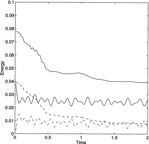
where KE 1 1 12 is the kinetic energy, PE = !F1 1 2 the potential energy,
R is the real part and r2 = k2 + 12 is the total (squared) wavenumber. The
nonlinear term on the right hand side permits transfer of energy between different wavenumbers, but does not alter the total energy, i.e.
R{* J( , 12')} = 0 (2.12)
k I
so that the sum over all wavenumbers of the sum of kinetic and potential energy is conserved, although of course there can be exchange of energy between the two components. Note that the nonlinear term derives solely from the advection of relative vorticity. In other words, there is no advection of thickness in the one and a half layer case, which is the same as saying there is no baroclinic instability (Pedlosky, 1987). The spectral transfer is mostly of interest in Chapter 4 since there is an active shift in scales due to turbulent interactions. In the case of the single vortex, the scales are essentially fixed so that the transfer is weak if not zero.
The conservation of PV also implies conservation of q" where n is any number. A frequently used quantity is the squared potential vorticity or the "potential enstrophy" (Charney, 1971). An equation for this quantity is found by multiply-ing equation (2.10) by q* = -(s2 + F1) * and then taking the real part of the
resulting equation:
81
11A"2
= -_{*J(1 ," )}. (2.13)Ot 2
The transfer on the right also vanishes when summed over wavenumber, so that the total enstrophy is conserved. Again note that changes in the quantity are
r-*err-- ~--~-C - ~.--~*C ^--.~l-L1*I~ -.- l.~ -l-I__-_~IYIUIIPPIX_-..^^^111.1 i
brought about solely by advection of relative vorticity. The addition of P changes neither conservation equation, (e.g. Rhines, 1977); however, with the addition of a bottom slope, enstrophy is no longer conserved in the lower layer.
The total energy for a two-layer flow is derived in a similar fashion. The Fourier-transformed upper layer equation (2.1) is multiplied by 60*/(1 + 8) and the transformed lower equation (2.2) by 0b/(1 + 8), the asterisk again indicating the complex conjugate. The real part of the sum of the resulting equations is:
tTE(r.) = V{)J(i, .201)} + -{2J(0 2, IC2?2)} + J(011{F , V)2)} (2.14) where TE = KE1 + KE2+ PE. The spectral transfers written in this way will be referred to as the "layer-wise" transfers because the first two terms derive from advection of relative vorticity in each layer. Note the first is the same as the transfer for the one and a half layer energy. The presence of a thickness transfer indicates the possibility of baroclinic instability (e.g. Salmon, 1980) when there is a correlation between temperature (thickness) and the perturbation velocity field (Pedlosky 1987). The sum over all wavenumbers of the transfers is zero, so again the total energy is conserved.
An alternate method, and one more commonly used with two layer models, is to break the total energy into barotropic and baroclinic parts (e.g. Salmon, 1980). One first adds and subtracts equations (2.1-2.2) to obtain equations for the barotropic and baroclinic vorticity. With equal layer depths, the result is (using the notation of Larichev and Held (1995)):
a--82
b + J(', V2 + 5) (7, + ,2 ( - -) = 0 (2.15)at(V
+ 2F)r + J(', 2T)+ J(r,V
2k)+
J(i, -2Fr) - #,2a ( - T) = 0 (2.16)where i =(~/i
+
+0 2) is the barotropic streamfunction and - - k2) thebaroclinic streamfunction. The energy equations follow after multiplying (2.15)
by b* and (2.16) by '*, and taking the real parts:
-. 2 = 2 )} J 2)} 2 {ik *f} (2.17)
RI{A *J(A, V J(
Q(I2+2F) " = {f*CJ( , 27 _R)}+I{f*J(k, -2FT)}+/82Rik0 *} (2.18)
The first transfer term in the barotropic equation represents barotropic self-advective changes and the second is due to transfers to/from the baroclinic mode. One finds that the sum over wavenumbers of the first is zero, but may be non-zero for the second as there may be a net exchange of energy between baroclinic and barotropic modes. Likewise, the first transfer term of the baroclinic equa-tion is the baroclinic self-advective term and the second the transfer to/from the barotropic mode, the sum of the first over wavenumbers being zero, but not nec-essarily zero for the second. However, the sum of the second term is the negative of the sum of the second barotropic transfer term, as is required by conservation of total energy. The two intermode transfers are not equal at every wavenumber as energy may be removed and injected at different scales (a striking example is found in Larichev and Held (1995)). The third baroclinic transfer term represents changes to the spectrum due to the advection of thickness by the barotropic field, and can be shown to be identical to the thickness transfer term in the total en-ergy equation (2.14). The final terms in both equations represent wave-induced transfers of energy between the barotropic and baroclinic modes. They cancel wavenumber by wavenumber, i.e. they are equal and opposite in the two budgets.
The barotropic/baroclinic formalism tends to be more illustrative of baroclinic instability, evidenced in particular by a conversion of baroclinic to barotropic energy. However, it will be seen that in cases of severe layer decoupling, the layer-wise transfers are preferable.
The equations for the two-layer potential enstrophies and transfers are found by multiplying equations (2.1-2.2) by q and q respectively, and taking the real parts:
S=
)}
(2.19)12 -_ 0{2J(2 q2)}- ,2_R{ikq2}. (2.20)
Again, the sum over all wavenumbers of the first transfer term in each equation is zero, implying conservation of the surface enstrophy in the absence of small-scale dissipation. But the lower layer enstrophy is not conserved due to the slope term (which need not sum to zero). The breaking of the conservation of enstrophy by topography has been noted before (e.g. Rhines, 1977). When the bottom is flat and dissipation present, the enstrophy monotonically decays in both layers.1
In forced-dissipative studies, the transfer terms are generally averaged over a long period because they tend to be noisy (e.g. Treguier and Hua, 1987; Larichev and Held, 1995). Averaging in time is less appealing for initial value problems because if the spectra are shifting in time, averaging tends to smear out the transfers. An alternative is to calculate the spectral fluxes, defined as :
'The equations shown here are inviscid, and thus do not represent the dissipation due to the filter. This could be done by adding a higher-order diffusion term. Then it would be clear that one obtains a monotonic decay of enstrophy.
flux(() = E trans
fer().
(2.21)The flux represents the net amount of energy entering or leaving the inner volume of wavenumber space. By virtue of being an integral quantity, the flux is less noisy than the transfer. It has the additional benefit of revealing immediately which terms have non-zero total integrals over all wavenumbers (the barotropic-baroclinic transfers). The spectral flux is by definition an isotropic quantity (averaged over all directions) and thus must be viewed cautiously in anisotropic flows. However, like the quadratic quantities in general, they provide a useful means of extracting information from the sometimes complicated flow fields.