Benchmark test problem for measuring anomalous dissipation in shock hydrodynamics simulations

by

Guy M. Snodgrass B.S., Computer Science United States Naval Academy, 1998

Submitted to the Department of Nuclear Engineering and the Department of Electrical Engineering and Computer Science in Partial Fulfillment of the Requirements for the Degrees of

Master of Science in Nuclear Engineering and

Master of Science in Electrical Engineering and Computer Science at the

Massachusetts Institute of Technology June 2000

© 2000 Massachusetts Institute of Technology. All Rights Reserved

Signature of Author ... ineering 5,2000 C ertified by ... I Molvig A6sociate Professor or C ertified b y ... klvin W. Drake nd Engineering Thesis Reader A ccepted by ... ... TT- Chen dents A ccepted by ... Arthur C. Smith MASSACHUSETTS !NSITUTE _{Chairman, Departmental Committee on Graduate Students}

OF TECHNOLOGY

JUL 3 1 2001

LARKER

Benchmark Test Problem for Measuring Anomalous

Dissipation in Shock Hydrodynamics Simulations

by Guy M. Snodgrass

Submitted to the Department of Nuclear Engineering and the Department of Electrical Engineering and Computer Science on May 5, 2000, in partial fulfillment of the requirements for the degree of Master of Science in Nuclear Engineering and

Master of Science in Electrical Engineering and Computer Science

ABSTRACT

Accurate simulation of strong compressions is a key capability needed in the design of efficient implosion systems. Anomalous dissipation due to the numerical hydrodynamics scheme can be an important limitation in the simulations, creating artificial (numerical) heat that reduces compression efficiency. This can inhibit using simulation to design efficient "adiabatic compression" schemes, for example. One obvious potential source of such anomalous dissipation is the fractional advection that occurs in Eulerian schemes where a portion of the mass, momentum and energy of the fluid is transported to neighboring cells. The advection fraction corresponds to what occurs in the continuum but inevitably spreads the field (mass, momentum, or energy) throughout the destination cell, effectively causing diffusion. When cell sizes exceed the physical mean free path, which is typically the case, diffusion produced by this effect will exceed the physical diffusion and anomalous dissipation can result. Various numerical corrections can be applied to mitigate this effect, but some residual effect is inevitable.

The purpose of this thesis is to define and demonstrate an unclassified benchmark test problem to determine the extent, if any, of such a dissipation anomaly. The particular cases are to be run using the Radiation Adaptive Grid Eulerian (RAGE) simulation code, developed at Los Alamos National Laboratory (LANL) in Los Alamos, New Mexico, USA. This code provides sophisticated strong shock hydrodynamics using an adaptive grid technology. The physical system devised as part of this thesis is a strong shock implosion modeled by two materials divided into three regions.

Strong compression can be accomplished by pushing a gas cavity to a smaller volume by means of a heavy bounding material, usually a spherical shell. In its simplest form, then, the problem is one in which a spherical shell, moving inward at some high initial velocity compresses the gas (and itself), until pressure buildup reverses the implosion. Although the actual results in practice depend on properties of the heavy material such as its strength and equation of state, the numerical anomaly of interest here is more general and can be expected to occur for any heavy material. By using a particularly simple heavy material we can expect to generate an adiabatic compression problem whose final state can be determined a priori, and yet can still be expected to show deviations due to anomalous numerical dissipation. In this way, we can separate the basic numerical issue from the detailed specific (and often classified) designs. This problem can serve as a benchmark test of any hydro scheme for the existence of anomalous dissipation, which is demonstrated in this particular test case. The numerical anomaly demonstrated in this thesis cannot be justified by the hydrodynamics of the system and is an artifact of anomalous dissipation within the hydrodynamics code.

Results are presented for a variety of simulations using a ID implementation of the spherical adiabatic code developed as a part of this thesis.

Thesis Supervisor: Kim Molvig

Title: Associate Professor, Nuclear Engineering Department Thesis Reader: Alvin Drake

Acknowledgements

This thesis would not have been possible without the research opportunity provided by my thesis advisor, Professor Kim Molvig. My thesis reader, Professor Al Drake, has been an excellent source of information and support throughout my course of study at MIT.

Many thanks also go to the team of scientists, engineers, and support staff at the Los Alamos National Laboratory. Among those with whom I interacted regularly were Mike Gittings, Bob Weaver, Bob Kares, Beverly Chavez, and Pam Paine. Their help was greatly appreciated and I hope to work with them again in the future.

I would also like to thank those at MIT who have helped me professionally as well as personally during my course of study: Clare Egan, Professor Neil Todreas, CAPT Matthew Lewis -US Army, Richard Williams, Leigh Heyman, Ben Wilson, Petr Swedock, Micah Smith, and Brendan Beer. Thank you all for putting up with me and for helping nonetheless.

Thanks also to those who provided words of advice, support, and encouragement while working on my thesis. Camilla Sulak, Professor Eugene Stanley of Boston University Physics Department, Shelley Fisher, Rachael Stanley, Professor Larry Sulak, Chairman of Physics at Boston University, and Dean Staton of MIT. All of you helped me look at the brighter side of life.

A great deal of appreciation goes to my mother, father and family for all of the moral support and encouragement while at the United States Naval Academy and MIT. Without your prayers this would not have been possible.

Amanda Johnsen has been a constant source of joy throughout my final year of study. Her constant encouragement and that of her family has been greatly appreciated. She is perhaps one of the most intelligent people I have ever met, and I am extremely lucky to have found her.

To those mentioned above as well as all of those who went unmentioned, your help was immeasurable. God Bless you all.

Biography of the Author

Guy Marvin Snodgrass was born on June 20, 1976 in Fort Worth, Texas. He graduated from Grapevine High School, Grapevine, Texas in May of 1994. He accepted a primary nomination to attend the United States Naval Academy in Annapolis, Maryland from the Honorable Joe Barton, United States Congressman, 6th District, Texas as a member of the Class of 1998.

While at the US Naval Academy he earned numerous academic honors, including induction into the Upsilon Pi Epsilon Computer Science Honor Society, Golden Key National Honor Society, Phi Kappa Phi Honor Society (for college seniors in the top six percent of their class academically), and multiple namings to the Superintendent's and Commandant's Lists (for superior academic and military performance). In February of 1998 he was selected to join the ranks of roughly 200 other classmates in service selecting Naval Aviation (Pilot) as his career choice. He was also awarded the Navy Burke Scholarship for post-baccalaureate study at the Naval Postgraduate School, Monterey, CA and an Immediate Graduation Education Program (IGEP) Scholarship for immediate two year post-baccalaureate study at a US university. He graduated as an Ensign in the top ten percent academically from the US Naval Academy on May 22, 1998.

Having been awarded full tuition at numerous educational institutions he chose to enroll at the Massachusetts Institute of Technology (MIT) in the Nuclear Engineering department as a Masters Candidate. While at MIT he petitioned for a Masters Degree from the Department of Electrical Engineering and Computer Science (awarded for fulfilling the requirements of both departments).

Upon leaving MIT he plans to begin his Naval Aviation training at NAS Pensacola, Pensacola, FL. ENS Snodgrass hopes to become an aircraft carrier pilot flying F/A-18 or F-14 fighter aircraft.

Table of Contents

A B ST RA C T

...

3

Acknow ledgem ents

...

5

Biography of the Author

...

7

1

Introd uctio n

...

11

1.1 O v erv iew ... 1 1 1.2 R esearch Inform ation ... 12

2

LANL RAGE Project...

15

2.1 R A G E O verview ... 15

2.2 Adaptive Mesh Refinement (AMR) Overview ... 16

3

Benchmark Test Problem Overview

...

19

3.1 G eom etrical Setup ... 20

3.2 Physics Derivation of Analytical Test Case... 22

4

Analytical Comparison of Test Case Results

...

31

4.1 Analysis of Primary Test Case (1mm sphere)... 31

4.2 Analysis of Second Test Case Results (4mm shell)... 45

4.3 Analysis of Third Test Case (2.5gm/cm2 _{shell density)...48}

5

Discussion of Numerical Anomaly

...

53

Appendix A

-

1mm Thick Shell Test Case

...

57

1

Introduction

1.1

Overview

Accurate simulation of strong hydrodynamic compression is a key capability needed in the design of efficient implosion systems. Anomalous dissipation due to the numerical hydrodynamics scheme can be an important limitation in the simulations, creating artificial (numerical) heat that reduces compression efficiency and inhibits the use of simulations to design efficient adiabatic compression schemes, for example. One obvious potential source of such anomalous dissipation is the fractional advection that occurs in Eulerian schemes where a portion of the mass, momentum and energy of the fluid is transported to neighboring cells. The advection fraction corresponds to what occurs in the continuum but inevitably spreads the field (mass, momentum, or energy) throughout the destination cell, effectively causing diffusion. When cell sizes exceed the physical mean free path, which is typically the case, diffusion produced by this effect will exceed the physical diffusion and anomalous dissipation can result. Various numerical corrections can be applied to mitigate this effect, but some residual is inevitable.

The purpose of this thesis is to define and demonstrate an unclassified benchmark test problem to determine the extent, if any, of such a dissipation anomaly. The particular cases are

to be run using the Radiation Adaptive Grid Eulerian (RAGE) hydrodynamics code, developed at Science Applications International Corporation (SAIC) by Mike Gittings and currently in use at Los Alamos National Lab (LANL). This code provides sophisticated strong hydrodynamics using an adaptive grid technology and copious use of the Message Passing Interface (MPI) for multiprocessor/multi-machine parallel support. More information on the RAGE hydrodynamics code is presented in Chapter 2.

1.2

Research Information

Much of the underlying research was performed during a summer internship at Los Alamos National Laboratory (LANL), one of the Department of Energy's premier national laboratories. Spending the entire summer of 1999 with LANL's Applied Theoretical and Computation Physics (X) Division presented the opportunity to work with excellent people and superior software tools required to complete this research. The people that collaborated on the physics design and setup for this project are amongst the best in the areas of simulation,

computational and nuclear science. The originator of RAGE, Mike Gittings of SAIC, is currently employed out of LANL and was more than happy to help design some of the early trial runs of various test simulations, including ID and 2D Sedov blast waves, shock tube tests and

Rayleigh-Taylor mixing. Bob Weaver, the team leader for RAGE at LANL, was also very helpful in teaching me how to work with and understand RAGE. Many other people working at both LANL and MIT helped with this project and they have my most sincere thanks.

The people who collaborated on this project are among the best, and the LANL X-Division is a premier resource in the United States for information, expertise and solutions for a wide range of nuclear physics and computing issues. It is this expertise that is driving the

development of the RAGE hydrodynamics code, the software program used at the Los Alamos National Laboratory to work on creating strong shock and other hydrodynamic simulations. Also important are the analytical tools used to extract data from the results, several of which were created at LANL. WShow, a Microsoft Windows@ compatible software program, was used

to analyze the TEK output files produced by RAGE (graphic xy-plot files). When more precision was necessary, Bob Kares' RAGE2ENS conversion program (UNIX OS) was used to interpret the output from RAGE into a form compatible with CEI's acclaimed EnSight visualization software. EnSight allows the user to manipulate data to produce plots of material variables and create animations of the graphical RAGE output. One can load a 2D compression problem and watch as the shell moves inward towards maximum compression.

Since RAGE itself has been a work in progress, several versions were used. The copy that was used most often was the 06131999 build of the code. Later, in the design of ID rectangular grid spaces, other more recent revisions were used, but as no data is included from those test runs it will not be necessary to document the other versions.

It should be noted that RAGE is a work in progress. As such the code was constantly evolving with new functionality available only towards the end of this research. Several test cases were designed that were not fully supported by the current RAGE development code. However, the cases represented here worked well with the RAGE hydrodynamics code in both the ID and 2D case.

2

LANL RAGE Project

Los Alamos National Labs is continuing its ongoing development of several methods that use computer programs for simulation purposes. Among one of the prominent programs is the RAGE hydrodynamics code. Developed by Mike Gittings at SAIC, RAGE (Radiation Adaptive Grid Eulerian) is a one, two and three dimensional multi-material Eulerian hydrodynamics code for use in solving a variety of high deformation flow of materials problems.

2.1 RAGE Overview

The DNA water shock program, specifically the modeling of underwater explosions in shallow water, helped influence the development of RAGE. During the development of this test series numerous one-dimensional calculations were performed to determine what codes or computational methods would best satisfy the demands of this problem. It was soon shown that two prominent features would be necessary: second order accuracy and an "adaptive grid" simulation. That is, the simulation code needed to be able to take a predefined cell and, if necessary, repeatedly divide it into multiple cells for greater accuracy and reduced numerical dissipation.

In the late 1980s an MLG (multi-material, piecewise Linear, Godunov) program was developed that met these requirements. At that time the MLG was a second order, multi-material Eulerian hydrodynamics code that was fully vectorized to run on Cray computers. In the MLG code the adaptive algorithm was designed to allow cells to be subdivided on a cycle-by-cycle and cell-by-cell basis. This allowed the computational grid to place cells exactly where needed in the geometrical representation framework. The MLG code has ultimately become what we now know as RAGE.

2.2

Adaptive Mesh Refinement (AMR) Overview

The RAGE simulation hydrodynamics code uses Adaptive Mesh Refinement (AMR) techniques to help reduce numerical dissipation and increase resolution in the simulation 'system.' This subsection is intended to provide an overview of AMR.

Typically a ID block has two cells, a 2D block has 4 cells, and a 3D block has 8 cells, as shown in Figure 2-1.

1

2

3 4

ID

1

2

2

Figure 2-1. Grid layout showing the AMR geometry of ID, 2D, and 3D cells.

The code orders and numbers the blocks but the numbering of the blocks is inconsequential as far as the user is concerned, since the input deck does not reflect the individual numbering of cells or blocks. All of the AMR and numbering techniques are carried out by the hydrodynamics code during a simulation cycle.

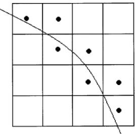
The first step is to define the problem set's grid "domain". The following is a simplified example of a 4x4 cell space that is cut by a line indicating a region of interest (as in our case with a metallic shell) or a change in a material property such as density, pressure, etc. The dots within the cell represent virtual markers that tell the code to subdivide those cells in the next cycle. The subdivision of cells continues until the line is located only in one cell of the block, or the maximum level of adaption is reached.

Figure 2-2. Example of 2D grid space bisected by Region of Interest (ROI)

The entire process is computed in parallel, unless only one processor is available, using the Message Passing Interface (MPI) as first created by Argonne National Lab. The number of cells per processor is entirely dependant upon the number of processors available. Addressing is on an internal/external basis. If the cells are located within the same processor the addressing is local, otherwise the addressing is external for communication between processors. This is the basic premise for the refinement of the grid space and division of cells amongst processors.

The majority of the code is written using Fortran90 with only a few high-level instructions written in C. The high-level C code performs three functions: decoding the argument string from the command line, enabling MPI with a different set of arguments

(available when run from C), and it calls the controller with the filename. The controller is the main processing unit, but there are several other modules that handle low-level coding and physics techniques. When the hydrodynamic program is run the controller steps through these modules, which perform a variety of functions. The rough pattern of execution is as a cycle. The subroutines initialize the problem, performs the "restart" process, performs an edit based on cycle number and time step, cycles through the simulation (t -> t + At ), and performs a

'cleanup'. During each cycle the program performs hydrodynamic, heat conduction, energy flow, radiation, and adaption calculations to influence the program's current state and next cycle. This is how a problem involving a moving substance is simulated: fractional calculations are performed to solve for the values in each cell for the next time step.

The RAGE hydrodynamic code is a very good package that works extremely well in a variety of situations. This thesis, however, seeks to demonstrate how the very small numerical dissipation inherent in hydro-code simulations can actually reduce the effectiveness of a real-world application. Chapter four describes how a very small dissipative effect can wind up costing a compression simulation to underpredict the adiabatic value by roughly 50%.

3

Benchmark Test Problem Overview

Strong inward compression can be accomplished by pushing a gas cavity to smaller volume by means of a heavy bounding material, usually a spherical shell. In its simplest form the problem is one in which a spherical shell, moving inward at some high initial velocity, compresses the gas (and itself), until pressure build up reverses the implosion. Although the results in practice depend on properties of the heavy material such as its strength and equation of state, the numerical anomaly of interest here is more general and can be expected to occur for

any heavy material. By using a particularly simple heavy material we can expect to generate an

adiabatic compression problem whose final state can be determined a priori, and yet can still be expected to show deviations due to anomalous numerical dissipation. In this way, we can separate the basic numerical issue from the detailed specific (and often classified) designs. The problem could serve as a benchmark test of any hydrodynamics scheme for the existence of anomalous dissipation.

The initial problem is to design and model a strong implosion. To accomplish this we use two different materials: a low-density gas and high-density, high-gamma material, also modeled as a gas. In this case, the model is made of a thin metallic region (approximated by the high-density, high-gamma (HDHG) material) being driven inward by its high initial velocity.

3.1

Geometrical Setup

The initial desired test case is described by a spherical gaseous cavity of low-density gas

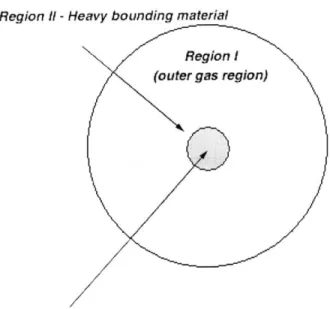
(Region III) that would be driven inward by a high-density bounding material (Region II). The higher-density bounding material would be surrounded by a large region of gas (Region I) at the same density and at a slightly higher pressure than that of the inner gaseous region. The following diagram demonstrates the initial test case schematic:

Geometrical Setup

Region 1 - Heavy bounding material Region I (outer gas region)

Region IIl -Inner gas region

Figure 3-1. Pictorial representation of gas and material regions

The geometrical layout of the simulation is subdivided into three material regions. The RAGE hydrodynamics simulation code requires the material boundaries to be defined in

inwardly progressing regions. This is why Region I is the outer most region and not the innermost.

The premise is to compress the (roughly) atmospheric inner gas Pg = 0.001 3 with

a heavy metal density material (PM =10.0 -3 to achieve (20)3 compression of the inner gas

and two to three fold compression of the metal shell. If we take representative physical dimensions to be 10cm for the inner gas radius and 0.1cm for the metal shell thickness, then the initial shell kinetic energy is set by the requirement of 8000 times adiabatic compression of the inner gas.

Once we have found the adiabatic conditions for the inner gas, the metal shell ratio of

specific heats, y,, can be determined such that it compresses the metal shell to 2.5 times its

initial density, assuming that adiabatic conditions hold throughout the process. To construct the simulation setup as demonstrated in Figure 3-1 we ascribe specific physical traits to each material region (density, specific internal energy, initial velocity, etc).

The outer region is composed of a low-density gas (0.001 g/cm3) of 50.0cm in radius that is at an initial pressure of 1,000 times atmospheric pressure (1.01x9 dynes/cm2). The second region is a thin, high-density (10.0 g/cm3)region of high-gamma (14.7) binding material that divides Region I and III from each other and was calculated to be able to adiabatically compress the inner gas region, Region III, inward to a radius of 0.5cm. The third region is the innermost region. The chart below better describes each region's material properties as set initially in the

3.2

Physics Derivation of Analytical Test Case

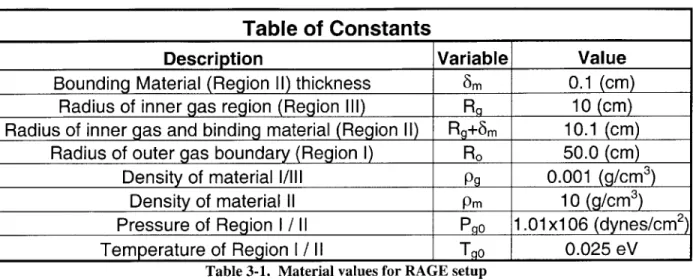
Table of Constants

Description Variable Value

Bounding Material (Region 11) thickness 6m 0.1 (cm)

Radius of inner gas region (Region Ill) RQ 10 (cm)

Radius of inner gas and binding material (Region 11) Rg+8m 10.1 (cm)

Radius of outer gas boundary (Region 1) Ro 50.0 (cm)

Density of material 1/Ill pg 0.001 (g/cm3₎

Density of material 11 Pm 10 (g/cm3₎

Pressure of Region I / 11 Pao 1.01x106 (dynes/cm)

Temperature of Region I / 11 Tqo 0.025 eV

Table 3-1. Material values for RAGE setup

The variable values required to initialize the RAGE input deck were calculated using the physics in this chapter. The physics were also calculated to reach certain adiabatic goals for compression of the metal and inner gas regions. Following is a discussion of the physics involved in this project. For a detailed numerical look at the equations with input properties, please see Appendix A.

In setting up our equations we first create certain parameters that we would like to achieve. One of the first is that we want to solve for an initial velocity that is sufficient to compress the inner gas region to 0.5cm.

R. 10cm(31

-

-20.0

Rf 0.5cm

As shown in equation (3.1) this decrease in radius corresponds to a 20 times compression of the inner gas. The metal shell must also have sufficient kinetic energy,

Eko = 4zR 2 I UO2 (3.2)

to provide the work done in compressing the gas in an adiabatic manner.

This requires the work in compressing the space to be derived, as follows:

W = PdV (3.3)'

where we express dV in radial geometry:

dV =4)7r 2dr (3.4)

The pressure at a given radius is adiabatically related to the original gas pressure (Pgo), initial density (p), final density (po) and ratio of specific heats (y) by equation 3.5:

/ \Y

P(r) = Pgo (3.5)

Pgo)

Instead of using the density of the material we can convert the equation to require only the ratio of specific heats, initial gas cavity radius (Rgo), and current radius:

P~r)= P Rgoy~

P(r)=go J (3.6)

Substituting equations (3.6) and (3.4) into (3.3) for pressure and volumetric compression, respectively, we yield the following result:

W = R947r2drPgo 0 93 (3.7)

R(

Equation series (3.8) walks through the process of solving this integrated form of work. Upon completion we have an easily solvable equation that relies on constants that we have already declared for the initial material conditions:

R9 W = PO 4 R, fdrr 2-3, Rf W = P 0 4rR3y r 3- 3y R, gO g 3 -3yR 3W3y RP 4 _{1 R9} W = R3 _{P II1} W = 4zR 9 P9 0 -3 yI - Rf

The pressure of the gas is a result of the product of the density of the gas and the thermal

2

velocity, cth

P = PgCth2 (3.9)

where: cth2 kT

m

Having previously stated that the metal shell's kinetic energy be sufficient to provide the work necessary to compress the inner gas we set (3.2) and (3.3) equal to each other:

Eko =W (3.10)

Substituting equation (3.2) for initial kinetic energy of the high-density material shell and equations (3.8) and (3.9) for work needed to perform the compression yields the following equation:

Rewriting (3.11) to solve for the initial velocity of the metal sphere yields:

2 2Rg Pg 2

U _{" 0} ~ ---_{3in PM}C

(y -1)K

R 3(y-1)

R) -1] (3.12)

With the initial conditions stated earlier in the chapter we have all the required variables to solve equation (3.12) with the exception of the thermal velocity. We also know that if

1

R = - R

20 g (3.13)

then the compression factor is:

1 (203(y-1))_1 ~ 100

Y - 1

(3.14)

for a gas region gamma, yg, of 1.5. We also already know that the ratio of the inner gas initial

radius to the initial metal shell thickness is:

Rg /S, ~ 102 (3.15)

and the ratio of the initial gas density (0.001 gm/cm3_{) to the initial metal region density (10}

gm/cm3_{) is:}

Pg

/PM

Using the above ratios it is reasonable to approximate that the initial metal shell velocity is equal to the thermal velocity:

uMO = C th (3.17)

In fact, after solving equation (3.12) numerically in Appendix A (A.4) we find that the initial metal shell velocity is in fact very close to the thermal velocity of the gas particles:

Un 0 =1.0859c,

(

An initial inward velocity of the metal is appropriate for the adiabatic calculation if it meets the following relationship to its Mach number:

M = uM2

<jCth

In this case the Mach number is 0.88, less than 1.0, justifying the value of umo for adiabatic compression.

Finding the relationship between the initial metal shell velocity and thermal velocity is important. However, RAGE requires the initial gas density, initial gas temperature, and specific heat at constant volume (c,) to initialize the gas regions. We can therefore use these to compute the thermal velocity and get initial metal velocity from Equation 3.18.

For an ideal gas the internal energy can be approximated knowing the degrees of freedom

Joules

(D), initial gas density, Boltzmann's constant (k = 1.38x10-23 ), mass of the gas particles

Kelvin

(m), and initial gas temperature (T):

D D D k

U = P = nkT = p -T = cT (3.19)

2 2 2 m

However, internal energy is also equal to the specific heat at constant volume times initial temperature. We can therefore use this information to solve (3.19) for the specific heat at constant volume:

C = p (3.20)

2 m

Earlier we stated that the ratio of specific heats, y, for the gas was 1.5. This was

estimated based on a standard near-ideal gas with four degrees of freedom. The ratio of specific heats can be calculated knowing the degrees of freedom as in (3.21):

D+2

y2 =(3.21)

Yg D

Earlier we related several constants to solve for the specific heat at constant pressure, but we can also use several of these values to solve for the thermal velocity:

T =_ c,2 (3.22)

Combining equations (3.20) and (3.22) we can solve for the thermal velocity:

2 2 c

Cth v T (3.23)

D pg

Using the result from (3.23) we can solve for the initial metal (and inner gas) radial velocity, (3.18). The result of that calculation (20,887.89cm/s) is presented in a table at the end of this chapter.

Now we also want an equation of state for the metal (high-density/high-gamma material) region such that the compression to achieve the final pressure results in a density compression of 2.5 times the original metal density. If we assume the metal pressure equals the gas pressure at maximum compression we can model the metal as an ideal 'gas' with a very high ratio of specific heats.

Pg = Pg = (20) pgo ~ 8000 pgo (3.24)

This is an important relationship, because if the simulation test case yields a result of 8.0 gm/cm3 _{for the final density of the inner gas we will have experienced adiabatic compression.}

Non-adiabatic compression would occur for a variety of reasons, but the result of which would produce losses that would reduce the effect of compression, therefore lowering the maximum density of the inner gas region.

Using (3.5) we can also solve for our ideal final inner gas pressure when undergoing adiabatic compression:

(

Pg > Pg =P Pg ~Pg (8000).5 ~(7.155x0Pgo (3.25)

Pgo)

According to (3.25) we can expect to see an increase in the pressure of the inner gas region at maximum compression on the order of 105. Assuming that the final pressure of the metal is equal to the final gas pressure we can say:

Pf = Pg = P.O '" (3.26)

P

P1

Also assuming that RAGE is initialized so that the initial metal and gas region pressures are equal:

r '

H

PnO Pgo)

Solving (3.27) for the ratio of specific heats for the metal yields:

In pg/ pgo Yg In (3.28)

'" =Y In p, lp.,n g In 2.5

Solving (3.28) then only depends upon the ratio of specific heats for the gas (1.5), the ratio of final gas density to initial gas density (8000), and the ratio of final metal density to initial metal density (2.5). The ratio of specific heats for the metallic material is therefore 14.7.

The pressure of a region can be equated to the ratio of specific heats, density, and specific

internal energy of that region, as shown in (3.29):

RAGE takes the specific internal energy (SIE), not pressure, to initialize a region. Therefore, rearranging equation 3.29 allows us to solve for the SIE of the region from the known value of pressure:

P

e = innergas (3.30)

Since out initial conditions require that the initial pressure in the inner gas region and the metallic shell be equal, we can solve for the SIE of the metallic shell by simply using the pressure of the inner gas region with the density (10.0 g/cm3) and ratio of specific heats (14.7) of the metal shell region:

P

eregionI "innergas (3.31)

The outer gas pressure is related using equation 3.25. This provides an outer gas pressure that will be equal to the adiabatic final inner gas pressure at maximum compression:

Poutergas = go (3.32)

= Pgo (20)

= Pgo (716,000)

A pressure jump of this magnitude would require special treatment at the interface and with a standard setup RAGE goes unstable numerically. Instead a value of 1,000 times Pgo is used to help hold the back of the material together. Note that this outer gas pressure is not really a part of the problem setup, but merely an artifice to eliminate outward expansion of the metal from its back surface. Any such backpressure will only enhance compression, in principle adding to the computed adiabatic density and pressure values. Using the same procedure as above, the outer gas specific internal energy is calculated:

outergas

region = (3.33)

Solving the entire sequence of equations for the desired adiabatic results is included in Appendix A for your convenience. Also included in this thesis is the RAGE input deck for the one-millimeter thick metal sphere compression test case, found in Appendix B. Included below is a list of the important variables solved in this chapter that are subsequently included in the RAGE input deck and that might change between different simulation test cases:

Variable Adiabatic Value Ratio of specific heats (yg) 1.5

Ratio of specific heats (Yin) 14.7 Specific heat at constant volume (cv,) 2.96x107 Specific heat at constant volume (cvm) 2.95x 10'

SIE Region I (outer gas) 2.02x1 012 erg/g

SIE Region II (metal shell) 7.37x103 erg/g SIE Region Ill (inner gas) 2.02x109 erg/g Density of gas (pg) 0.001 g/cm3 Density of metal (pm) 10 g/cm3 Metal shell velocity (uro) -2.09x1 03 cm/s

4 Analytical Comparison of Test Case

Results

The test cases were run remotely on LANL's theta and tO] remotely accessible computer clusters. The results were output in two separate forms: TEK plot files, which are black and white xy-plot representations of the material properties, and DMP files, which are text output files that RAGE saves to the hard drive at each output time step. The DMP files can be converted, using Bob Kares' RAGE2ENS program, into a format that is compatible with CEI's EnSight 6.2/7.0 analysis toolkit. EnSight allows a user to manipulate data to create various custom plots and to easily compare the data. The majority of the data contained within this thesis is provided in TEK format since it is more easily manipulated.

4.1

Analysis of Primary Test Case (1mm sphere)

The first test case was also the benchmark for all other subsequent test cases. Here the RAGE setup mirrored what has been presented in the previous three chapters. We expect to see results like those presented in Table 3.1. For example, the initial metal density is 10.0 gm/cm3,

and at maximum compression (an inner gas radius of 0.5cm) the expected result is for the metal

region to compress to 2.5 times its initial value, or 25.0 gm/cm3

The following paragraphs detail the experimental results of the 1mm thick spherical

compression test case. The major predicators of performance are plots of: pressure, density,

temperature, material, and fractional volume. Using the data from these figures the

determination can be made as to how close the hydrodynamic code comes to achieving adiabatic

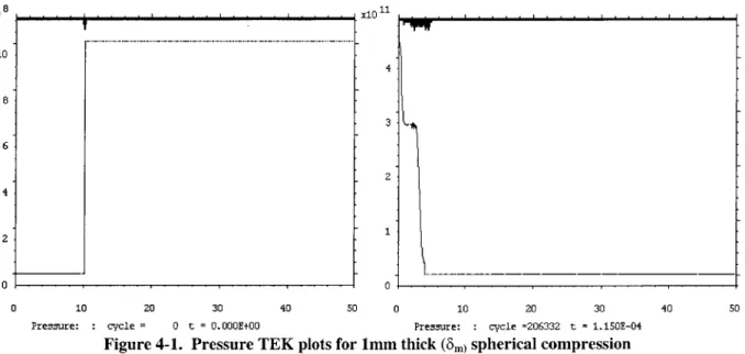
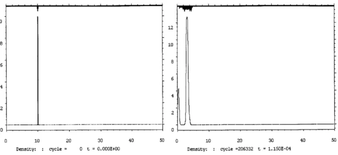
compression. x10 . . . ._ 1 __._._._. 10 4 8 3 6 4 2 0 0 2 0 10 20 30 40 50 0 10 20 30 40 50

Pressure: cycle = 0 t = 0.OOOE+00 Pressure: cycle =206332 t = 1.150E-04

Figure 4-1. Pressure TEK plots for 1mm thick (8m) spherical compression

As Figure 4-1 demonstrates, the final maximum compression occurs at approximately

t=1.15x 10-4 sec. _{The right-hand side plot also shows that the final experimental inner gas} pressure does not equal the expected adiabatic result. If the compression process had been

adiabatic the final inner gas pressure would equal the result of (A.19) which is 7.23x10 1

dynes/cm 2. Instead, the actual experimental result yielded 4.30x 10" dynes/cm2, which is

10 12 8 ₁₀ 8 6& 4 4 2 2 0 0, 0 10 20 30 40 50 0 10 20 30 40 50

Density: cycle = 0 t = 0.000E+00 Density: cycle =206332 t = 1.150E-04

Figure 4-2. Initial and final density for 1mm test case

Figure 4-2 displays the initial density condition for the three material regions at initialization (t = 0.0s). Remember that initially there are three material regions. The third region extends to a radius of 10.0cm and has a density of 0.001 g/cm3. The second region extends from 10.0 to 10.1 cm and has a density of 10.0 g/cm3, which appears as a solid bar in the left-hand plot. The outermost region extends from 10.1cm to 50.0cm and has the same density as Region III. The plot on the right-hand side displays the density for the inner gas and metal sphere at maximum simulated compression. According to the initialization parameters (second paragraph of Appendix A) the final density for the inner gas would be 8.0 gm/cm3 and for the metal sphere is 25.0 g/cm3 _{under adiabatic conditions. The simulation results again underpredict} maximum density with an inner gas density of 4.28 g/cm3 (46.5% lower than adiabatic) at

maximum compression. The metal sphere increases its maximum density from 10.0 gm/cm3 to 12.8 g/cm3_{, (48.8% lower than predicted adiabatic). The analytical density for the inner gas was} calculated based on a maximum compression of the gas to 0.5cm. The expected density for an adiabatic compression to 0.6cm is:

(Rg . (10.0cm 3

pg = Pg 0.cm) Pgo ~ 4629.63po = 4.6 gm / cm 3 (4.1)

gf=Rgf 0.6cm)

The results from the experimental test case show a density very close to this value.

Therefore it is probable that the density has reached near-adiabatic compression.

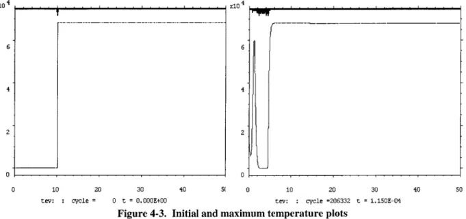
The temperature plots are useful in this situation for two reasons: the initial conditions

can be easily error checked, and the error present in the pressure and density values might be

attributed to an effect found within the maximum compression plot.

x10 x104 6 6 4 4 2 2 0 0 0 10 20 30 40 5( 0 10 20 30 40 50

tev: cycle = 0 t = 0.000E+00 tev: cycle =206332 t = 1.150E-04 Figure 4-3. Initial and maximum temperature plots

The initial plot looks correct, but to ensure accuracy EnSight was used to find the exact

values for temperature in the different regions, as demonstrated in later figures. In Appendix A

we show that for the inner gas the pressure was initially 1.01x106 dynes/cm2 _{and the temperature}

was 0.025 eV (1/4 0 h an eV is approximately room temperature). The temperature plot at

maximum compression shows that a region of unusually high temperature and low density is

found between 0.6cm and 2.0cm. This heating of the gas could be one reason why the 'hole'

exists within the density plot of Figure 4-2. The temperature will be very useful later in this

2.0 2.0 1.8 1.8 1.6 1.6 1.4 1.4 1.2 1.2 1.0 1.0 0 10 20 30 40 50 0 10 20 30 40 50

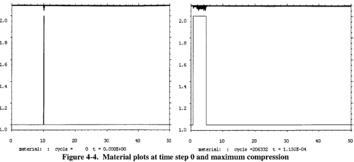
material: cycle = 0 t = 0. 000E+00 material: cycle =206332 t = 1.150E-04

Figure 4-4. Material plots at time step 0 and maximum compression

The material plots in figure 4-4 represent the radius of the total sphere that the different materials occupy. For instance, the material for the inner and outer gasses is represented as material '1.0'. This reflects the input in the RAGE setup file, as shown in Appendix B, where material one is set up as the gas in material regions I and III. The low-density gas is therefore set up as material '1.0' and the high-density gas region (Region II) material is setup as material '2.0.' The initial plot therefore corresponds exactly with the initial density view: this is because upon initialization (time step 0) the entire material 2.0 region is located in the high-density region. This is another good indication that the initial run-time conditions were properly set in the RAGE input deck.

The material plot at maximum compression reveals something interesting about the material regions. The material plot shows an extension of the second material from approximately 0.6cm to 4.9 cm, a large area. This would indicate that the material has spread 50 fold from its original value of 0.1cm. The expected spreading of the shell under adiabatic conditions is 2.86cm as shown by Equation 4.2 when the inner gas is compressed to 0.6cm:

4 (R,03 - Rg₀3 )Pjo = (R - R g 3 p, (4.2)

This represents the spreading of the material assuming constant density at the value, pmf,

corresponding to the adiabatic pressure and conservation of mass. In this case there is a region of mixed material extending roughly from 0.6cm to 2.5cm which will be discussed later in the chapter.

The plot in Figure 4-4 will be even more useful after the discussion on the fractional

volume plot for material number two.

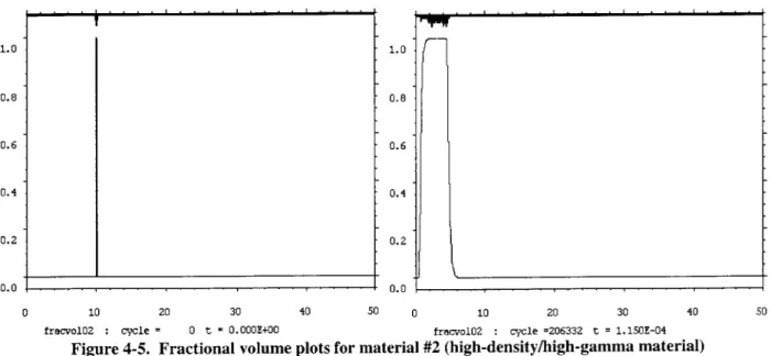
1.0 1.0 0.8 0.8 0.6 0.6 0.4 0.4 0.2 0.2 0.0 0.0 0 10 20 30 40 50 0 10 20 30 40 50

fracvol02 cycle = 0 t = 0.OOOE+00 fracvol02 cycle =206332 t = 1.150E-04 Figure 4-5. Fractional volume plots for material #2 (high-density/high-gamma material)

Noticing the previous non-adiabatic behavior in the pressure, density, and temperature plots the material and fractional volume plots provide a wealth of important information. The fractional volume plots serve a similar purpose as the material plots, with the distinction that the material plots reflect the position of a 50% mix of the material. If 50% of material two exists in

the cell, the material plot considers it to be wholly of material two. Conversely, the fractional volume plot equates a value of '1.0' if the cell at that location along the radius is wholly of material two, a value of 0.0 if wholly of material one, and a fraction thereof if only partially material two. For example, at a radius of 1.0cm the fractional volume is approximately 0.5,

37

signifying that that at a distance of 1cm from the center of the sphere there are equal parts of material one and material two.

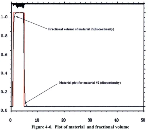
The real usefulness of the plots is in the ability to use a tool such as Adobe PhotoshopTM

to overlay the fractional volume plot with the material plot at time step zero and also at maximum compression, as in Figure 4-6.

1.0

Fractional volume of material 2 (discontinalty)

0.8

0.6

0.4

Material plot for material #2 (discontialty)

0.2

0.0

0 10 20 30 40 50

Figure 4-6. Plot of material and fractional volume

The overlay of the material and fractional volume plots make apparent that at maximum compression the two do not overlap completely. What this reveals is that mixing of the two working fluids is occurring at the leading and trailing edge of the high-gamma material sphere as it implodes. One of the most important side effects is that the mixing makes it extremely difficult to determine where the material two inner boundary ends. The material plot indicates that the inner bound of material two is at approximately 0.6cm. The fractional volume plot, however, reveals that at a 50% level of material two the fractional volume boundary is at the material boundary, but to reach a cell that contains all material two means moving further from

the center to approximately 1.75cm. The difference in final compression radius makes a very large difference in the expected final density of both the inner gas and metal (high-gamma material) shell.

Under Variable Initial value Expected value Actual value prediction

Inner gas radius (R.) 10.0 cm 0.5 cm 0.6 cm 20%

Metal shell thickness (8m) 0.1 cm n/a 4.0 cm n/a

Inner gas density (p.) 0.001 gm/cm3 _{8.0 gm/cm}3 _{4.28 gm/cm}3 _46.50%

Metal shell density (pm) 10 gm/cm3 25.0 gm/cm3 12.8 gm/cm3 _48.80%

Inner gas pressure (P.) 1.01x106 dynes/cm27.23x1011 dynes/cm2 4.3x1011 dynes/cm2

40.50% Meta region pressure (Pm) 1.01x106 dynes/cm2 n/a 2.75x1011 dynes/cm2 _n/a

Table 4-1. Change in values for test case variables

The data in Table 4-1 presents an overview of the initial values, the expected values at

maximum compression (adiabatic), the actual experimental result, and the error.

Underprediction was calculated by:

jExpected - Actualj

Underprediction = xl 100% (4.3)

Expected

With the exception of inner gas radius, almost all of the underpredictions hover around

50%, a consistent result that indicates the experiment results from the RAGE hydrodynamics

code are approximately half of the analytical adiabatic expectation. This behavior, lack of

adiabatic compression, can be explained by several mechanisms.

First, the use of any Eulerian hydrodynamics code with a rectangular cell space will have

a hard time arriving at the exact adiabatic answer. The reason for this lies in the linear method of

travel for a vector as well as the possibilities for numerical anomalies in the mass, momentum,

and energy of the material traveling between cell spaces. In a simulation code the cells are of

finite size, which causes the mass, momentum, and energy of the adjacent cells to prematurely

hydrodynamics code the transport of mass, momentum, and energy will not be perfect. This will be expressed in greater detail shortly.

Another reason for underprediction from the adiabatic case is the material interface. This simulation was planned using physics that took a high-gamma/high-density material as the binding spherical material. In the real application the binding material would be more likely to compress and increase in density rather than spread as quickly as seen here. One reason for the spreading and anomalous results is that both materials were initialized as gases (as the simulation

represents them). This could potentially allow the two materials to interface and rapidly begin to mix as the second region (the thin metallic shell) moves inward. This mixing unbalances the results providing two regions, one directly in front of Region II and one on the trailing edge of Region II, that are a mixture of gas materials one and two. This mixing creates a new heterogeneous gas that is a combination of the first two. This reasoning and that of the previous paragraph can be shown in the following sequence of plots produced in EnSight:

Frame 00 (Initial Conditions) Temperature

Density Pressure Temperature

0

9

93

10

10.5-Distance (cm)

In Figure 4-7 the initial conditions are presented using a plot illustrating the initial metal

shell density (10.0 g/cm3), temperature of the outer gas region (= 6,000eV), and pressure

(1.01x106 dynes/cm2 _{in the inner region and metal shell and 1.01x10}9 _dynes/cm2 _{in the outer gas}

region). The following sequence of plots shows the progression of the shell compression as it nears maximum compression (which occurs in time step 23).

Frame

02

9

9.5

10

10.5

Distance (cm)

Figure 4-8. Time step #02 after initiating simulation run

Figure 4-8 shows the plot of temperature, pressure and density at the second time output time step (RAGE was configured in the input file to output plots at constant time intervals, which is every 5.0x10-6 seconds, as shown in Appendix B). At this frame we see the pressure gradient progressing through the metal sphere, which is represented here by the area of high density. The curvature of the pressure plot in the metallic region indicates expansive behavior in the metal except for the leading edge, which appears compressive.

The curvature of the pressure gradient can typically be characterized as compressive, expansive, or neutral. A straight line (i.e. no curvature) indicates a neutral pressure profile and the material is not expanded or compressed in a hydrodynamic manner. If the pressure profile is concave relative to the direction of movement this indicates a compressive profile. The material that is in this region would therefore tend to compress. Finally, if the pressure profile is convex (bowing outward) relative to the direction of movement this indicates an expansive profile and the material is likely to expand in thickness.

Figure 4-8 then makes sense because the metal has to expand to conserve mass as it is compressed inward because the surface area of the inner and outer surfaces of the shell are reducing. This holds true unless the density rises appreciably in the metal region, which is what we expect to see based on our criteria that the density of the metal increase to 25.0 g/cm3.

Time step #06

Density Pressure Temperature Deinsity Pressure 0

8.4

8.6

8.8

9.0

9.2

9.4

9.6

Distance (cm)

Figure 4-9 illustrates the relative positioning of the three curves after six plots have been

produced (t

=

Time step

#20

~ -Density Pressure Pressure Temperature Density 0

3.5

4

4.5

5

5.5

Distance (cm)

Figure 4-10. Time step #20 plot

Figure 4-10 shows a steep rise in the pressure despite several scaling changes (numerical

values for the y-axis are not included to prevent confusion between the three material variables as EnSight renders them unreadable). The simulation has now proceeded for 1.Ox 104 seconds. The pressure profile in Figure 4-11 now exhibits a maximum within the high density metal region indicationg an outward force on the back half of the metal while still accelerating inward on the inward half. This is the beginning of pressure gradient reversal that will signal the reflection of the incoming shell. It is also a highly expansive form of pressure profile.

Figure 4-11 demonstrates that as the compression process nears maximum compression the pressure plot reverses, effectively causing the shell to slow down and bounce after maximum compression. The plots also illustrate that there is no hydrodynamic reason for the inner surface

of the metal to spray inward towards the inner gas. The two materials are mixing only slightly, and as we will describe soon this causes large problems with our particular compression test case.

Time step #22

0

1

2

3

4

Distance (cm)

Figure 4-11. Plot of time step #22

The plot also shows a rise in the temperature of the region between 0.8cm and 2.1cm. This corresponds with the region of gas/metal mixture residing between the compressed inner

gas and the inner surface of the metal shell. The temperature 'spike' will be even more evident in Figure 4-12, which illustrates the profile and relative values of temperature, pressure, and density at maximum compression.

The change in time between time step #22 and time step #23 is the same as all other frames. One important detail to visually recognize is that the inner gas region radius changes significantly between the two frames but the inner radius of the metal shell is nearly constant.

This indicates that there is some sort of buffer that is keeping the metal shell from continuing the compression inward, and is perhaps causing premature reflection.

Time step #23 (max)

Pressure Temperature

Density

0

0

1

2

3

4

Distance (cm)

Figure 4-12. Plot of temperature, density, and pressure at maximum compression

The reason for not achieving adiabatic behavior can be attributed to the region of high temperature just behind the inner gas region, which indicates a process that has taken place that hinders compression. This was hinted at earlier in this subsection when the issues of numerical anomaly and the rectangular grid were cited as potential non-adiabatic compression. This region corresponds to the mixed region of gas in the interface boundary between the inner surface of the Region II sphere and the Region III inner gas. As the plots illustrates, in conjunction with the earlier fractional volume TEK plots, is that as the shell compresses inward some of the metal on the inner surface of the shell is ejected into the inner gas region due to extremely small numerical artifacts. This forms a new 'hybrid' mixed region that maintains a low density similar to that of the inner gas region but mixes other properties of the metal and gas, such as the ratio of specific

heats, Ym and yg. This hybridization causes the new region to be nearly incompressible. In this

case an attempt to compress the mixed gas region results not in a pressure and density rise but instead in a spike in the temperature. This inherently points to a region of non-adiabatic compression caused by a very small numerical anomaly. Normally the mixing of the gas regions would be a small issue on the whole, but in this case the temperature is related by:

T oc p '- (4-4)

Despite the low density of the compressed region (compared to the metal shell) the attempt to compress this material at such a high gamma number (14.7) results in a large rise in the temperature.

This is a very good indication that the incompressible region cannot be explained due to hydrodynamic causes.

4.2

Analysis of Second Test Case Results (4mm shell)

The second test case arose from the desire to attempt to construct a test case that would yield a simulation that produces results closer to the adiabatic analytical case. The test case and input (reference Appendix C and Appendix D for physics and input file, respectively) for this test case are almost the same as for the 1mm thick shell compression case. The difference is that the shell thickness was increased by a factor of four, in the hopes that the thicker shell boundary would result in greater adiabatic compression. In order to adapt the physics of the new

1 1

simulation case to remain adiabatic the initial metal shell velocity is decreased by --,f4 2

which still yields a final compression radius of 0.5cm, a 8000x compression of the inner gas density, and a 2.5x compression of the metal shell density.

x10 8 Initial Condition X1 10 Mavim unm Ciompression

10 12 10 8 8 6 6 4 4 2 2 0 0 0 10 20 30 40 50 0 10 20 30 40 50

Pressure: : cycle = 0 t = 0.000E+00 Pressure: : cycle =378832 t = 2.050E-04 Figure 4-13. Pressure plots for 4mm thick shell simulation

Figure 4-7 shows the pressure plots for the 4mm thick shell case at the initiation of the run and at the point of maximum compression, t = 2.05x10-4 s. The expected adiabatic result is 7.23x 101 dynes/cm2 (for compression of inner gas to 0.5cm), the maximum compression pressure for the inner gas from the 1mm shell is 4.3x101 dynes/cm2, and the pressure at maximum compression for the 4mm thick spherical shell is 1.2x101 dynes/cm2

. 10 15 8 10 6 4 5 2 0 --- 0-- 0 10 20 30 40 50 0 10 20 30 40 50

Density: : cycle = 0 t = 0.OOOE+00 Density: : cycle =378832 t = 2.050E-04 Figure 4-14. Density plots for 4mm thick shell simulation test case

Figure 4-8 shows mixed results. The inner gas density at maximum compression has fallen to approximately 2.25 gm/cm3. However, the metal density error has improved, with the density rising from around 12.0 gm/cm3 to a little over 15.0 gm/cm3. The redesign of the 1mm thick shell test case to a 4mm thick shell test case was to try to arrive at experimental results that are closer to the adiabatic case in Appendix A. The main predicator of this is the density of the metal shell, thus we can claim a significant improvement (an 8% reduction in error). An even thicker shell case might prove beneficial but would move away from real-world cases.

4 .. Initial Condition 4 Maximu1iii I C.Imnpresion

x1__x10 _6_._._._._ _10 6 6 4 4 2 2 0 0 0 10 20 30 40 50 0 10 20 30 40 50

tev: cycle = 0 t = 0.OOOE+00 tev: cycle =378832 t = 2.050E-04

Figure 4-15. Temperature plots for 4mm thick shell

The temperature plots represented in Figure 4-9 still show a spike in the temperature of the mixed material region at a radius of approximately 1.5cm. The temperature of this spike, however, has decreased from a previous value of 6.0ev in the 1mm thick shell case to 3.9eV in this case. This reduction, coupled with the reduction of error in the metal density at maximum compression, indicated an increase in the adiabatic performance of this simulation test case.